https://doi.org/10.5194/amt-10-4697-2017 © Author(s) 2017. This work is distributed under the Creative Commons Attribution 4.0 License.
A more representative “best representative value” for daily total
column ozone reporting
Andrew R. D. Smedley, John S. Rimmer, and Ann R. Webb
Centre for Atmospheric Science, University of Manchester, Manchester, M13 9PL, UK
Correspondence to:Andrew R. D. Smedley ([email protected]) Received: 8 June 2017 – Discussion started: 13 July 2017
Revised: 20 October 2017 – Accepted: 20 October 2017 – Published: 5 December 2017
Abstract. Long-term trends of total column ozone (TCO), assessments of stratospheric ozone recovery, and satellite validation are underpinned by a reliance on daily “best repre-sentative values” from Brewer spectrophotometers and other ground-based ozone instruments. In turn reporting of these daily total column ozone values to the World Ozone and Ul-traviolet Radiation Data Centre (WOUDC) has traditionally been predicated upon a simple choice between direct sun (DS) and zenith sky (ZS) observations. For mid- and high-latitude monitoring sites impacted by cloud cover we dis-cuss the potential deficiencies of this approach in terms of its rejection of otherwise valid observations and capability to evenly sample throughout the day. A new methodology is proposed that makes full use of all valid direct sun and zenith sky observations, accounting for unevenly spaced observa-tions and their relative uncertainty, to calculate an improved estimate of the daily mean total column ozone. It is demon-strated that this method can increase the number of contribut-ing observations by a factor of 2.5, increases the sampled time span, and reduces the spread of the representative time by half. The largest improvements in the daily mean estimate are seen on days with the smallest number of contributing direct sun observations. No effect on longer-term trends is detected, though for the sample data analysed we observe a mean increase of 2.8 DU (0.82 %) with respect to the tradi-tional direct sun vs. zenith sky average choice. To comple-ment the new calculation of a best representative value of to-tal column ozone and separate its uncertainty from the spread of observations, we also propose reporting its standard error rather than the standard deviation, together with measures of the full range of values observed.
1 Introduction
Global ground-based monitoring of total column ozone (TCO) relies on the international network of Brewer spec-trophotometers since they were first developed in the 1980s (Kerr et al., 1981), which has expanded the number of sites and measurement possibilities from their still-operating predecessor instrument, the Dobson spectrophotometer. To-gether these networks provide validation of satellite-retrieved total column ozone as well as instantaneous point measure-ments that have value for near-real-time low-ozone alerts, particularly when sited near population centres, as inputs to radiative transfer models at ultraviolet wavelengths, and crit-ically underpin the monitoring requirement of The Vienna Convention for the Protection of the Ozone Layer, 1985.
The majority of the effort spent on calibrating Brewer spectrophotometers is directed towards ensuring high-quality DS calibrations are distributed globally through the Brewer reference triad (Fioletov et al., 2005), through the intercom-parisons at the Regional European Calibration Centre, and through initiatives such as COST Action ES1207 and EU-BrewNet. ZS observations are then linked to the DS cali-bration through a polynomial fit of quasi-synchronous DS and ZS observations (Kipp & Zonen, 2005). This additional calibration step explains the default preference for DS over ZS measurements as it incurs a small associated uncertainty. However, at mid- and high-latitude stations in particular the annual mean cloud fraction can exceed 50 % (Wilson and Jetz, 2016) and limits opportunities for recording vi-able DS observations. As a consequence, for a high fraction of days the best representative daily value (BRDV) is based upon zenith sky measurements. More crucially during partly cloudy days, the BRDV can be reliant on a small number of individual DS observations (< 5), which may be biased to-wards either the start or end of the day, whilst a greater num-ber of valid ZS observations from throughout the observation period are rejected
This gives rise to the question: could a more representative daily value be obtained from an increased number of ZS mea-surements than from a small number of DS meamea-surements? To answer this still forces a choice between valid DS and ZS observations as the number of DS measurements falls – whichever set of observations is chosen, a set of otherwise valid data is not incorporated into the calculation of the best representative value. Therefore, we propose an alternative methodology to calculate a best daily representative value that retains both direct sun and zenith sky measurements, taking into account their relative uncertainties and periods of time when valid measurements are more frequent.
2 Instrument and data processing description
Brewer spectrophotometers, their operation, and standard data processing routes have been described previously in the literature (Brewer, 1973; Fioletov et al., 2005; Smed-ley et al., 2012; Savastiouk and McElroy, 2005). For con-text we outline the key points here. The core of each instru-ment is a single or double monochromator unit whose out-put is detected by a photomultiplier tube. For the DS mea-surement mode the input is from a rotating prism assembly pointed towards the sun’s disc. Column ozone observations are achieved by rapidly repeated measurements at five opera-tional wavelengths over a period of approximately 3 min, and a final value is calculated by implementing the Lambert–Beer law and knowledge of the absorption cross section of ozone molecules. ZS observations are made in the same way but the rotating prism is instead directed to collect scattered light from the zenith, and then an empirical polynomial adjust-ment is applied. This polynomial adjustadjust-ment assumes that
the apparent ozone column from the zenith sky measure-ment is quadratic in both the air mass factor and the ac-tual column ozone. The nine constants necessary are deter-mined from a large number of quasi-simultaneous DS and ZS measurements (> 500) and are instrument and site specific. This relationship is usually determined at the instrument’s home site, rather than during an intercomparison or calibra-tion exercise, though Fioletov et al. (2011) described an im-proved radiative-transfer-modelling-based methodology that reduced the instrument-specific unknowns to two parame-ters (though nine constants are still necessary). However the polynomial constants are determined, the ZS observation is then found by solving the relevant quadratic equation.
3 A more representative daily value
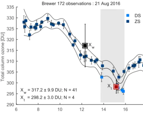
For a site where direct sun can be guaranteed for the major-ity of the day, an instrument could be scheduled to only at-tempt DS observations at regular intervals (together with the necessary diagnostic routines) and the mean of these obser-vations would be a reliable estimate of the actual daily mean TCO overhead at the station. For other sites where cloud is more variable and unpredictable, the observational schedule must contain a combination of both ZS and DS measure-ments. However, local cloud cover conditions may only per-mit a small number of DS measurements to be successfully recorded. Figure 1 shows an example day where only four DS observations were recorded between 13:48 and 15:49 UTC and where their arithmetic mean (298.2 DU) differs substan-tially from the daily mean TCO at the station as indicated by ZS observations. In order to avoid the potential binomial choice between a small number of DS observations and a greater number of ZS observations, we propose a weighted daily mean that utilises all valid DS and ZS values.
Our aim is to construct a daily mean that has the following properties. In the absence of either any valid DS or ZS obser-vations, it produces the same result as the standard method (once clustering of observations is accounted for). With the addition or subtraction of a single DS data point, there is a graceful change in the BRDV and the overall time period it represents. It should represent as fully as possible the day’s TCO observations. It should give equal weight to equal pe-riods of time and hence account for time clustering of valid observations and for their relative uncertainties. It should be able to be applied to historic data and not necessitate any changes to the instrument’s future schedule or data collec-tion routines.
over-6 8 10 12 14 16 18 UTC Time [h]
290 295 300 305 310 315 320 325 330 335
Total column ozone [DU]
Brewer 172 observations : 21 Aug 2016
Xw
Xt X = 317.2 ± 9.9 DU; N = 41w
X = 298.2 ± 3.0 DU; N = 4t
DS ZS
Figure 1.Example day showing valid DS and ZS observations and their standard deviations. Also shown are the daily representative value based on the traditional (arithmetic mean, DS > ZS prefer-ence) methodology (red outlined square,Xt)and the daily repre-sentative value formed through the method described herein (black outlined square,Xw). The shaded area shows the time coverage for data points contributing to the traditional estimate of the BRDV, and N is the number of contributing observations to each BRDV estimate.
all DS–ZS bias= −0.4 DU and the standard deviation of dis-tribution of individual DS–ZS pairs=6.3 DU).
All DS and ZS measurements are then filtered to remove those that do not meet the validity criteria. Observations that have a standard deviation of > 2.5 DU for DS and > 4.0 DU for ZS are rejected. We note that the standard choice of stan-dard deviation threshold is 2.5 DU for ZS observations, but increasing the limit to 4 DU does not introduce any bias and increases the total number of valid observations (Fioletov et al., 2005, 2011). Observations at air mass factors > 4 are also rejected for single monochromator instruments, but this limit is raised to 6 for double monochromator instruments due to their improved stray light rejection (Karppinen et al., 2015). To ensure that any residual bias is not present at high air mass factors, an additional tail removal step is applied. For this the day’s data are smoothed with a 30 min running average filter, and end periods of time where the smoothed TCO exhibits apparent rates of change > 20 DU h−1are identified. Any ob-servations falling within these periods are then removed.
At this stage the remaining DS and ZS values meet the specified validity criteria and have passed the additional tail removal check. To form a BRDV from these individual ob-servations, we calculate a weighted mean of the full set of data points but where the weighting has two components: the time for which the observation is representative and the
un-certainty of each observation, as in Eq. (1):
X= P
i
Xiwi
P
i
wi
, (1)
whereXis the BRDV,Xiis the individual observations (both
DS and ZS), andwi is the weighting for each observation.
The weighting is defined in Eq. (2) as wi=
ti
σi2, (2)
wheretiis the time from the midpoint of the preceding
inter-observation time interval to the midpoint of the following inter-observation time interval. For the first data point we in-stead use the length of the first inter-observation time period, and likewise for the last data point. In all casesσi is the
un-certainties for each individual observation, taken as the nor-mal measurement standard deviation and used as part of the validity test. If no account were to be taken of the relative uncertainties of each observation or of their time intervals, this formulation would reduce to the simple arithmetic mean of the valid observations.
We also note that this methodology could be applied to all data acquired without applying a threshold standard devia-tion validity filter as data points with large errors will con-tribute to the BRDV proportionally less. However, more care needs to be taken as regards relaxing the air mass threshold requirement as small biases may be introduced, inflated by the effect of observing at high air mass, whilst the uncertainty would not have been captured by the intrinsic standard devi-ation of the observdevi-ation. Further the ZS uncertainties could be expanded appropriately to account for any day-to-day bias between ZS and DS observations under differing sky condi-tions or alternatively to incorporate the DS–ZS polynomial fit mean residual, for example.
For higher-latitude sites where other measurement modes are relied upon, such as focussed moon, focussed sun, or TCO derived from global spectral irradiance, these observa-tions could also be incorporated into the BRDV calculation in a similar way (see seasonal variation of observation types in Karppinen et al, 2016). The prerequisites would be that each individual observation should have an associated uncer-tainty and that the observations from different measurement modes should be homogenised beforehand. In terms of prac-tical implementation, if the method were adopted by the com-munity a new observation type would have to be registered at WOUDC (a mechanism that is already available), with rele-vant details added to the scientific support statement as nec-essary. For stations that submit raw data, or processed indi-vidual observations, the weighted mean BRDV calculation could be applied across all sites as a daily summary value.
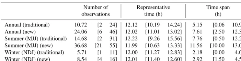
Table 1.Summary statistics for data shown in Fig. 2: number of contributing observations, representative observation time, and time span of contributing observations. For each case, values shown are the arithmetic means, and in brackets the lower 10th percentile and upper 10th percentile values are shown.
Number of Representative Time span
observations time (h) (h)
Annual (traditional) 10.72 [2 24] 12.12 [10.19 14.24] 5.15 [0.06 10.94]
Annual (new) 24.06 [6 46] 12.02 [11.01 13.02] 7.61 [2.50 12.35]
Summer (MJJ) (traditional) 14.68 [2 31] 12.22 [9.26 15.56] 7.76 [0.50 12.25] Summer (MJJ) (new) 36.68 [21 55] 11.99 [10.63 13.33] 11.56 [10.00 13.00] Winter (NDJ) (traditional) 5.71 [1 11] 12.00 [11.27 12.83] 2.18 [0.00 4.00]
Winter (NDJ) (new) 8.54 [4 16] 12.01 [11.40 12.60] 2.92 [1.50 4.50]
gradient present, then the most appropriate daily measure should return a value similar to the TCO above the site. The traditional method risks producing a daily value that could be substantially different if, due to cloud cover, only a few valid DS measurements could be recorded during early morning or late in the day when the TCO is being sampled to the west or east of the site. In partly cloudy or cloudy conditions a minimum air mass TCO measurement may not be obtained. In contrast, the proposed method guards against these issues as ZS observations could be sampled more fully through the day, whilst the contribution from DS measurements would represent the effective TCO along the slant path when the di-rect solar beam is visible. As a result the proposed BRDV TCO calculation is more appropriate for UV exposure stud-ies than the traditional calculation, more representative of the conditions throughout the day, and more resilient than rely-ing on a srely-ingle value at minimum air mass, for example. For non-linear spatial gradients in TCO, the limited DS measure-ments could result in a value more different still from the mean TCO overhead, while the bias from the selection of the TCO near minimum air mass would depend on the spatial distribution of ozone.
4 Sample results
To demonstrate the impact of this method on real world data, we apply it to the 2000–2016 data record from Brewer spec-trophotometer #172, located in Manchester, UK (53.47◦N, 2.23◦W) (see Table 1 and Fig. 2). For context the minimum air mass observed at this location during the summer solstice is approximately 1.15, whilst during the winter solstice it is 4.15.
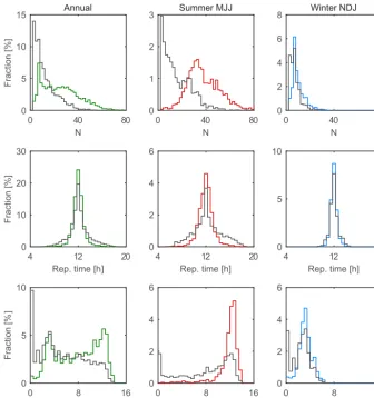
Overall we see an increase in the mean number of con-tributing observations (N) from 10.72 to 24.06, with the up-per 10th up-percentiles also increasing from 24 to 46. The ef-fect is dominated by summertime measurements that show an increase of 150 % from 14.68 to 36.68 averaged over the 3 months bracketing the summer solstice. Whilst the effect is still present during winter months (when data collection is inherently more difficult due to the lower solar elevations),
the improvement is smaller: the meanNincreases from 5.71 to 8.54 contributing observations per day.
As expected we see concomitant tightening of the distri-bution of representative times (defined as the mean of valid observational times, weighted by their TCO values) around solar noon (close to midday). There is also a skewing of the observational time span distribution to longer periods. The representative time is symmetrical about solar noon in both the traditional and new methods, but the width of the annual distribution (defined as the interdecile range) is halved from 4.05 to 2.01 h, showing the new method results in BRDVs that are more representative of the conditions at solar noon. Again due to the longer day length the improvement is accen-tuated during summer (6.5 h reduced to 2.7 h) but still present during winter months (1.56 h reduced to 1.20 h). Time spans for the whole year are generally skewed to the right-hand side of the distribution, though the upper and lower bounds do not change (being limited by number of daylight hours and instances of single contributing observations respec-tively). Much of the skewness in the annual distribution is at-tributable to that occurring during the summer subset (Fig. 2, third row, second column), where the lower 10th percentile increases from 0.5 to 10.0 h.
Taken together these results demonstrate that the method enables a more representative daily mean to be calculated, predominantly by sampling more fully through each day and over a wider range of weather conditions. However, it is pru-dent to investigate the impact on the overall time series and trends.
differ-0 40 80 N
0 5 10 15
Fraction [%]
Annual
0 40 80
N 0
1 2
3 Summer MJJ
0 40 80
N 0
2 4 6
8 Winter NDJ
4 12 20
Rep. time [h] 0
10 20 30
Fraction [%]
4 12 20
Rep. time [h] 0
2 4 6
4 12 20
Rep. time [h] 0
5 10
0 8 16
Time span [h] 0
5 10
Fraction [%
]
0 8 16
Time span [h] 0
2 4 6
0 8 16
Time span [h] 0
2 4 6
Figure 2.Histograms of the number of contributing observations (N, first row), representative observation time (second row), and time span of contributing observations (third row) for 2000–2016 for all months (first column), summer months (May–June–July, second column), and winter months (November–December–January, third column). Grey traces show results from the traditional method, and coloured traces show results for the methodology described in the present study.
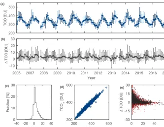
ent instruments immediately after calibration), and with the upper and lower 10th percentiles being−2.67 and 10.92 DU respectively (equivalent to−0.79 and+3.22 % of the annual mean TCO). The methodology does not substantially alter the form of the time series with anR2 coefficient of 0.984 (Fig. 3, lower middle panel). It should be emphasized that this bias of 2.79 DU does not result from the ZS polynomial procedure, nor is it related to any bias between individual DS and ZS measurements: the overall bias of the polyno-mial fit is only−0.4 DU. Instead the bias noted here relates to the new method’s increased sampling over longer daylight hours. The underlying cause is likely related to a longer sam-pling period where the TCO is larger or to increased reliance on different internal filters. We anticipate that the former is dominant as Fig. 3 (middle panel) suggests increased differ-ences during summer months when the time span is increased the most.
200 300 400 500
TCO [DU]
2006 2007 2008 2009 2010 2011 2012 2013 2014 2015 2016 2017 Year
-10 0 10 20 30
∆
TCO [DU]
-40 -20 0 20 40 ∆ TCO [DU] 0
10 20 30
Fraction [%]
200 400 600
TCOt [DU] 200
400 600
TCO
n
[DU]
0 20 40 60 No. DS obs -30
-15 0 15 30
∆
TCO [DU]
(a)
(b)
(c) (d) (e)
Figure 3. (a)Traditional monthly mean TCO; line length shows the upper and lower monthly 10th percentiles.(b) Mean monthly daily difference between the new and traditional best representative values plus the upper and lower monthly 10th percentiles.(c)Histogram of daily differences between traditional and new daily TCO calculations.(d)Scatterplot of new daily TCO values against the traditional TCO. (e)Scatterplot of daily difference between the new and traditional BRDV against the number of contributing DS measurements; dark grey markers are for data points from months JJASON, red markers are from the remainder.
Together these results suggest that there should be no im-pact on long-term trends at a site where the data record is derived from a single instrument type. However, there could be implications where there has been a change in the data sampling method. Moving from a semi-manual Dobson spec-trophotometer that makes a limited set of observations on a predefined schedule to a Brewer spectrophotometer that op-erates quasi-continuously and selects a daily value on the traditional DS vs. ZS choice could introduce a small step change due to this effect, which may contribute to a perceived trend. Likewise applying the proposed method to only part of a data record, because individual historical measurements have been lost, for example, could also introduce a small step in the overall record.
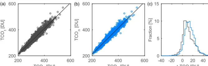
Testing the influence of the new methodology in terms of the agreement between ground-based and satellite retrievals (Fig. 4), we find a marginal improvement in the ground vs. satellite TCO for daily mean data in terms of their R2 cor-relation (0.9560 vs. 0.9455) and best fit slope (1.0041 vs. 0.9930). More noticeably, there is a narrowing of the distri-bution of differences (ground minus satellite) from an inter-decile range of 26.86 to 24.01 DU, whilst the mean is shifted to higher biases (from 10.49 DU under the traditional DS– ZS preference to 13.28 DU). Satellite retrievals were also compared against the closest individual observation to the
overpass time under two assumptions. First, by selecting the nearest valid DS measurement as a preference, and if none were available, then by selecting the closest ZS observation (equivalent to the traditional DS–ZS choice). Second, by se-lecting the closest observation to the mean overpass time with no preference for observation type (equivalent to the proposed BRDV calculation). The results nonetheless were very similar to those for BRDV in Fig. 4.
5 Measures of daily spread and estimating real-time TCO
While the focus of this study is on the determination of a more representative daily TCO value, there are a number of related issues concerning reporting of the daily spread that will be discussed in this section.
200 400 600 TCOs [DU] 200
400 600
TCO
t
[DU]
200 400 600
TCOs [DU] 200
400 600
TCO
n
[DU]
-40 -20 0 20 40 60 ∆ TCO [DU] 0
5 10 15
Fraction [%]
(a) (b) (c)
Figure 4. (a)Traditional BRDV with traditional DS–ZS choice vs. Ozone Monitoring Instrument (OMI) mean overpass.(b)BRDV from described methodology vs. OMI mean overpass.(c)Histogram of daily differences between traditional (grey) and new (blue) daily TCO calculations vs. satellite overpass TCO.
hypothesis for this test is that the individual daily observa-tions come from a standard normal distribution, and on ap-plication we find that this null hypothesis is not rejected for any of the days in our test sample. That is, all can be consid-ered as being taken from a normal distribution.
Whilst this result does not undermine the use of the stan-dard deviation as a measure of the spread of the day’s data, we propose that other metrics may be more useful. Specifi-cally, to separate out the uncertainty in the best representative daily value from the range exhibited by individual observa-tions, a more useful measure would be to use the standard error of the weighted mean to indicate the uncertainty of the best representative value plus additional metrics relating to the maximum and minimum TCO observed. The latter could be the strict maximum and minimum, or, to guard against the influence of short-duration spikes, the upper and lower 10th or 25th percentiles could be used, for example.
Whilst developing the methodology described in Sect. 3, the geostatistics analysis route known as “kriging”, or Gaus-sian process regression, was also tested (Bailey and Gatrel, 1995; Lophaven et al., 2002). This analysis produces the best linear unbiased estimator of the actual underlying TCO at times intermediate to the observations and also produces an associated uncertainty. In brief, it performed well for days where there are a larger number of contributing observations but showed poorer performance during winter or other days with few observations. This latter issue is in part due to the complex nature of applying the method, where for few ob-servations there is a risk of overfitting. However, for studies where short-term prediction of the TCO and its near-term un-certainty is of interest, such as real-time estimates or now-casting, kriging may find applications. More generally its applications could include spatial analysis and interpolation of TCO and surface irradiance, which are two fields where global datasets are reliant on a limited number of measure-ment sites.
6 Conclusions
In this study, we propose, describe, and assess a new method-ology for determining a more representative best daily value of total column ozone from Brewer spectrophotometer ob-servations. This method overcomes the limitations of mak-ing the traditional choice between a possibly small number of direct sun measurements and zenith sky measurements. It requires a homogenised set of DS and ZS data as a prerequi-site but then, by taking a weighted mean and accounting for both the uncertainty associated with each individual observa-tion and the time period the observaobserva-tion represents, produces a more representative value based on the full set of daily ob-servations.
Applying the new method to the 2000–2016 dataset from Brewer 172 stationed at Manchester (53.47◦N, 2.23◦W), we show that the number of contributing observations is more than doubled from an average of 10.72 to 24.06 per day; increased numbers of observations are found in both sum-mer and winter, though the fractional increase is greater during the summer. Similarly the interdecile range of mean representative times is approximately halved throughout the year, whilst the time span of contributing observations is skewed towards longer hours, predominantly during the sum-mer months. Together these findings demonstrate that the method results in a substantial improvement in sampling and utilisation of valid observations and hence improves the rep-resentativeness of the daily mean TCO. The issue of rejecting otherwise valid data is also removed. We find no evidence of impact on supra-annual trends from the application of the new method, though the ground-satellite bias is increased for this station by 2.8 DU. We also note that a change in daily sampling when one instrument type replaces another at a site could contribute to the introduction of a small step in the data record, and, similarly, care should be taken if reprocessing only a partial data record.
limits of the interdecile range, or simply the maximum and minimum observed values.
Data availability. The underlying data used in this study can be
ac-cessed at the World Ozone and Ultraviolet Radiation Data Centre (Smedley et al., 2017).
Author contributions. ARDS was primarily responsible for the data
collection, processing, and monitoring of Brewer spectrophotome-ter #172 and led the manuscript preparation. JSR assisted with data collection, contributed to the manuscript, and secured funding. ARW contributed to the manuscript, secured funding, and was the Principal Investigator on the overall grants.
Competing interests. The authors declare that they have no conflict
of interest.
Acknowledgements. Stratospheric ozone and spectral UV baseline
monitoring in the United Kingdom is supported by DEFRA, the Department for Environment, Food, and Rural Affairs, since 2003. The authors would also like to thank Vladimir Savastiouk and two anonymous referees for their constructive and valuable comments.
Edited by: Andrew Sayer
Reviewed by: Vladimir Savastiouk and two anonymous referees
References
Bailey, T. C. and Gatrel, A. C.: Interactive spatial data analysis, Addison-Wesley, 1995.
Brewer, A. W.: A replacement for the Dobson spectropho-tometer? Pure Appl. Geophys., 106–108, 919–927, https://doi.org/10.1007/BF00881042, 1973.
Fioletov, V. E., Kerr, J. B., McElroy, C. T., Wardle, D. I., Savastiouk, V., and Grajnar, T. S.: The Brewer reference triad, Geophys. Res. Lett., 32, L20805, https://doi.org/10.1029/2005GL024244, 2005. Fioletov, V. E., McLinden, C. A., McElroy, C. T., and Savas-tiouk, V.: New method for deriving total ozone from Brewer zenith sky observations, J. Geophys. Res.-Atmos., 116, 1–10, https://doi.org/10.1029/2010JD015399, 2011.
Karppinen, T., Redondas, A., García, R. D., Lakkala, K., McElroy, C. T., and Kyrö, E.: Compensating for the ef-fects of stray light in single-monochromator Brewer spec-trophotometer ozone retrieval, Atmos. Ocean, 53, 66–73, https://doi.org/10.1080/07055900.2013.871499, 2015.
Karppinen, T., Lakkala, K., Karhu, J. M., Heikkinen, P., Kivi, R., and Kyrö, E.: Brewer spectrometer total ozone column measure-ments in Sodankylä, Geosci. Instrum. Method. Data Syst., 5, 229–239, https://doi.org/10.5194/gi-5-229-2016, 2016.
Kerr, J. B., McElroy, C. T., and Olafson, R. A.: Measurements of ozone with the Brewer spectrophotometer, in Proceedings of the Quadrennial International Ozone Symposium, edited by: Lon-don, J., Natl. Cent. for Atmos. Res., Boulder, Co., 74–79, 1981. Kipp & Zonen: Brewer Mk III spectrophotometer operator’s
man-ual, Delft, 131 pp., 2005.
Lophaven, S. N., Nielsen, H. B., and Søndergaard, J.: DACE: A MatLab Kriging toolbox, Report IMM-TR-2002-12, Informat-ics and Mathematical Modelling, DTU, 28 pp., available at: http://www2.imm.dtu.dk/projects/dace/dace.pdf (last access: 4 November 2016), 2002.
Massey Jr., F. J.: The Kolmogorov-Smirnov test for goodness of fit, J. Am. Stat. Assoc., 46, 68–78, 1951.
Savastiouk, V. and McElroy, C.T.: Brewer spectrophotometer to-tal ozone measurements made during the 1998 Middle Atmo-sphere Nitrogen Trend Assessment (MANTRA) campaign, At-mos. Ocean, 43, 315–324, https://doi.org/10.3137/ao.430403, 2005.
Smedley, A. R. D., Rimmer, J. S., Moore, D., Toumi, R., and Webb A. R.: Total ozone and surface UV trends in the United Kingdom: 1979–2008, Int. J. Climatol., 32, 338–346, https://doi.org/10.1002/joc.2275, 2012.
Smedley, A. R. D., Rimmer, J. S., and Webb, A. R.: UK ozone and UV monitoring site no. 352, WOUDC, https://doi.org/10.17616/R32C87, 2017.
Wilson, A. M. and Jetz, W.: Remotely sensed high-resolution global cloud dynamics for predicting ecosystem and biodiversity distributions, PLoS Biol., 14, e1002415, https://doi.org/10.1371/journal.pbio.1002415, 2016.
WMO (World Meteorological Organization): Scientific Assessment of Ozone Depletion: 2014, World Meteorological Organization, Geneva, Switzerland, 416 pp., 2014.