OMI tropospheric NO 2air mass factors over South America: effects of biomass burning aerosols

(1)

www.atmos-meas-tech.net/8/3831/2015/ doi:10.5194/amt-8-3831-2015

OMI tropospheric NO

2

air mass factors over South America: effects

of biomass burning aerosols

P. Castellanos1,a,b, K. F. Boersma2,3, O. Torres4, and J. F. de Haan2

1_{Faculty of Earth and Life Sciences, VU University Amsterdam, Amsterdam, the Netherlands} 2_{Royal Netherlands Meteorological Institute (KNMI), De Bilt, the Netherlands}

3_{Meteorology and Air Quality Group, Wageningen University, Wageningen, the Netherlands} 4_{NASA Goddard Space Flight Center, Greenbelt, MD 20771, USA}

a_{now at: NASA Goddard Space Flight Center, Greenbelt, MD 20771, USA} b_{now at: GESTAR/Universities Space Research Association, Columbia, MD, USA}

Correspondence to: P. Castellanos (patricia.castellanos@nasa.gov)

Received: 16 January 2015 – Published in Atmos. Meas. Tech. Discuss.: 12 March 2015 Revised: 9 June 2015 – Accepted: 22 August 2015 – Published: 18 September 2015

Abstract. Biomass burning is an important and uncertain

source of aerosols and NOx(NO+NO2)to the atmosphere. Satellite observations of tropospheric NO2 are essential for characterizing this emissions source, but inaccuracies in the retrieval of NO2 tropospheric columns due to the radia-tive effects of aerosols, especially light-absorbing carbona-ceous aerosols, are not well understood. It has been shown that the O2–O2 effective cloud fraction and pressure re-trieval is sensitive to aerosol optical and physical proper-ties, including aerosol optical depth (AOD). Aerosols im-plicitly influence the tropospheric air mass factor (AMF) calculations used in the NO2retrieval through the effective cloud parameters used in the independent pixel approxima-tion. In this work, we explicitly account for the effects of biomass burning aerosols in the Ozone Monitoring Instru-ment (OMI) tropospheric NO2 AMF calculation for cloud-free scenes. We do so by including collocated aerosol ex-tinction vertical profile observations from the CALIOP in-strument, and aerosol optical depth (AOD) and single scat-tering albedo (SSA) retrieved by the OMI near-UV aerosol algorithm (OMAERUV) in the DISAMAR radiative transfer model. Tropospheric AMFs calculated with DISAMAR were benchmarked against AMFs reported in the Dutch OMI NO2 (DOMINO) retrieval; the mean and standard deviation of the difference was 0.6±8 %. Averaged over three successive South American biomass burning seasons (2006–2008), the spatial correlation in the 500 nm AOD retrieved by OMI and the 532 nm AOD retrieved by CALIOP was 0.6, and 68 % of

(2)

1 Introduction

Satellite observations of backscattered radiation have been vital in measuring and monitoring global-scale air pollution, consisting of a mixture of aerosols and reactive gases that are either directly emitted or formed through various chemi-cal and physichemi-cal processes. These global data sets of atmo-spheric composition contain important information on the chemistry of the atmosphere (e.g., Stavrakou et al., 2013), trends in air quality (e.g., Castellanos and Boersma, 2012), as well as emissions from fossil fuel burning (e.g., Jaeglé et al., 2005), biogenic hydrocarbon sources (e.g., Marais et al., 2012), lightning (e.g., Bucsela et al., 2010), and biomass burning (e.g., Castellanos et al., 2014). However, the retrieval of tropospheric column amounts of trace gases from satellite observations is complicated and remains a challenge.

In the retrieval of NO2tropospheric columns, air mass fac-tors (AMFs) are used to derive vertical columns from slant columns that have been calculated from a DOAS (differential optical absorption spectroscopy) fit to measured radiances or reflectances. The tropospheric AMF is calculated with a ra-diative transfer model and accounts for the difference in the sun-to-satellite photon path within the troposphere (the slant column) versus the vertical path from a ground pixel to the top of the troposphere. The AMF is the dominant source of error in retrieving NO2 tropospheric columns for polluted scenes (Martin, 2002; Boersma et al., 2004) and depends strongly on observable parameters such as the surface albedo, satellite viewing geometry, terrain height, and the presence of clouds and aerosols, as well as assumed parameters such as the NO2 profile shape. All of these aspects can give rise to large errors in the AMF calculation and the retrieved NO2 tropospheric column for individual measurements. In this pa-per, we will focus on how aerosols, specifically emitted by biomass burning, affect tropospheric AMFs.

In the Dutch OMI NO2(DOMINO) retrieval (Boersma et al., 2011), as well as DOAS-based retrievals for other instru-ments and species such as formaldehyde (De Smedt et al., 2012) and ozone (Van Roozendael et al., 2006), the indepen-dent pixel approximation is used to account for the presence of clouds. Thus, the AMF is taken to be a linear combination of a clear-sky AMF and a cloudy-sky AMF.

M=wMcl+(1−w) Mcr (1)

w= feffIcl

feffIcl+(1−feff) Icr

(2) In Eq. (1), M is the tropospheric AMF, Mcl and Mcr are the cloudy- and clear-sky AMFs, respectively, andw is the radiance-weighted cloud fraction (or simply radiance cloud fraction) (Eq. 2); a function of the effective cloud fraction is denoted by feff;Icl andIcr are the fit window averaged radiances for 100 % cloudy and clear scenes, respectively (Boersma et al., 2004).

The DOMINO retrieval does not directly take into account the effect of aerosols on the AMF, but instead uses an implicit

correction by assuming that the cloud parameters retrieved by the OMI (Ozone Monitoring Instrument) cloud algorithm (OMCLDO2) (Acarreta et al., 2004; Stammes et al., 2008) account for the effect of the aerosols on the light path. The DOMINO retrieval takes the approximation that the effects of aerosols on the tropospheric AMF can be represented as the fractional coverage of a Lambertian reflector that yields a top-of-atmosphere (TOA) reflectance that best agrees with the observed reflectance, i.e., a radiometrically equivalent, or effective, cloud fraction. Previous work has shown that for OMI the effective cloud fractions retrieved in the O2–O2 band are indeed sensitive to aerosols; retrieved cloud frac-tions were higher and cloud pressures were lower in the pres-ence of aerosols compared to a pure molecular scattering at-mosphere, and aerosol optical depth (AOD) was strongly cor-related with effective cloud fraction, especially for strongly scattering aerosols (Boersma et al., 2004; Boersma et al., 2011). Lin et al. (2014) showed that the presence of aerosols can lead to lower or higher cloud pressures depending on the aerosol height, cloud height, and aerosol optical properties.

For a few synthetic cases of assumed aerosol type and opti-cal depth, Boersma et al. (2004) showed that the tropospheric AMF could increase by as much as 40 % when aerosol radia-tive effects are directly accounted for. This raises the follow-ing question: to what extent can the implicit correction via the retrieved cloud parameters mimic the effects of differ-ent observed aerosol concdiffer-entrations, vertical aerosol distri-butions, and physical aerosol properties?

Compared to a pure molecular scattering atmosphere, the presence of a scattering component, whether aerosol or cloud, can change light paths as well as their contributions to the TOA reflectance. In some aspects, the radiative ef-fects of scattering aerosols and clouds are comparable. Both aerosols and clouds decrease the sensitivity to an absorber at lower altitudes, as more photons will be scattered back to the satellite before reaching the surface, a shielding effect. Moreover, clouds and aerosols also increase the sensitivity to an absorber above the scattering layer, by increasing the contribution of these light paths to the TOA reflectance, i.e., an albedo effect. While these effects can be approximated by the effective cloud model, an opaque Lambertian sur-face with high albedo (Koelemeijer and Stammes, 1999) (i.e., the altitude-dependent AMFs (Eskes and Boersma, 2003) or scattering weights (Palmer et al., 2001) below a cloud are zero), aerosols can modify the radiative transfer in ways that may not be adequately covered by this model.

(3)

different characteristic sizes (cloud particles being larger), aerosol and cloud particles have different phase functions. Thus, an accurate estimate of the height and physical prop-erties of an aerosol layer with respect to the vertical distribu-tion of the absorber is essential for accurate air mass factor calculations for trace gas retrievals (Leitão et al., 2010).

Lin et al. (2014) studied the effect of aerosols on OMI NO2tropospheric column retrievals at three urban/suburban MAX-DOAS measurement sites in eastern China by im-plementing aerosol optical depth (AOD) from AERONET or MAX-DOAS observations, and aerosol physical proper-ties (single scattering albedo (SSA) and phase function) and vertical profiles from the GEOS-Chem chemical transport model in the AMF calculation, and explicitly corrected the O2–O2cloud retrieval for the presence of aerosols. With their aerosol-corrected O2–O2cloud parameters, and in situations with the AOD exceeding 0.8, their tropospheric AMF was significantly higher than the DOMINO v2 retrieval, and the NO2tropospheric column was 70–90 % lower when aerosol effects are included. However, when averaged over 30 days, the explicit correction for aerosols resulted in NO2 tropo-spheric columns that were only 14 % lower than the original DOMINO v2 retrieval.

In this work, we investigated the properties of the implicit aerosol correction for tropospheric NO2retrievals from OMI in the case of active biomass burning in South America, which generates elevated concentrations of reactive gases and aerosols. South America contributes on average approxi-mately 5 % of total global annual burned area, but 15 % of to-tal global annual biomass burning carbon emissions (Giglio et al., 2010; van der Werf et al., 2010) are due to the high fuel loading and combustion completeness of deforestation burning along the borders of the Amazon. Bottom-up esti-mates of biomass burning NOxemissions are largely

uncer-tain due to unceruncer-tainties in the static emission factors used to convert biomass consumed into NOx emitted. New

param-eterizations based on top-down estimates of NOx emissions

from OMI NO2 observations have been proposed as a way to better characterize the variability in biomass burning NOx

emission factors (Mebust et al., 2011; Schreier et al., 2014). In this paper, we focus on areas of active burning to analyze whether the effects of aerosols on NO2tropospheric AMFs could influence these top-down estimates.

In our analysis we compared NO2 tropospheric AMFs from the DOMINO v2 algorithm to AMFs calculated with explicit aerosol scattering and absorption in the radiative transfer calculations. To describe the aerosol optical prop-erties in the AMF calculations, we utilized measurements of AOD and SSA retrieved from simultaneous OMI mea-surements in the UV (OMAERUV algorithm; Torres et al., 2013), as well as collocated aerosol extinction vertical profile measurements from the Cloud-Aerosol Lidar with Orthogo-nal Polarization (CALIOP) instrument (Winker et al., 2010). While previous studies have relied on models or ancillary point measurements, such as MAX-DOAS or AERONET,

to analyze the effects of aerosols on tropospheric NO2 re-trievals, our approach is novel in that it exploits globally available satellite measurements. This allows for the analy-sis of the OMI data record over large spatial and temporal scales, and potentially for a globally consistent observation-based explicit aerosol correction.

2 Satellite observations and radiative transfer

modeling

2.1 The Ozone Monitoring Instrument (OMI)

OMI is a nadir viewing imaging spectrometer aboard the EOS Aura satellite that measures backscattered radiation in the UV–Vis from 270 to 500 nm (Levelt et al., 2006). Dur-ing the first 3 years of operation startDur-ing in 2004, OMI provided daily global coverage at a nominal resolution of 13 km×24 km for nadir pixels. In mid-2007, what is prob-ably an external obstruction began affecting the quality of the radiance observations of all wavelengths at specific view-ing angles. Each viewview-ing angle corresponds to a row on the OMI 2-D CCD detector. Hence, the degradation of the OMI data quality for some viewing angles is referred to as the row anomaly. Currently, approximately half of the sensor’s view-ing angles are affected by the row anomaly (Braak, 2010).

2.2 OMI effective cloud fraction and cloud pressure

retrieval (OMCLDO2)

The O2–O2effective cloud fraction formulation assumes the observed TOA reflectance between 460 and 490 nm can be represented by a linear combination of the cloudy- and clear-sky fractions of the pixel (Eq. 3), where the cloud is modeled as an opaque Lambertian reflector with albedo equal to 0.8 (Acarreta et al., 2004; Stammes et al., 2008).

R=feffRalbedo=0.8+(1−feff) Rcr (3) In Eq. (3), R is the simulated reflectance best matching the observed reflectance,feff is the effective cloud fraction, Ralbedo=0.8 is the simulated reflectance for a Lambertian cloud with albedo equal to 0.8, andRcris the simulated clear-sky reflectance. A cloud albedo of 0.8 was chosen to compen-sate for the missing transmission of the opaque Lambertian cloud model (Stammes et al., 2008).

The retrieval spectral window includes the collision-induced absorption feature of oxygen (O2–O2)at 477 nm. In the presence of clouds, O2–O2 complexes below the cloud are shielded, and because oxygen is well mixed, the observed O2–O2slant column is a measure of the height of the cloud.

(4)

pressure with the aid of a look-up table (LUT) produced with the doubling–adding KNMI (DAK) v3.0 radiative transfer model. In the retrieval, the surface albedo for the simula-tion of the clear-sky reflectance is taken from the Kleipool et al. (2008) climatology.

O2–O2 absorption is a function of the square of the O2 number density. As a consequence, the TOA radiance mea-sured by OMI is a function of the inverse of the tempera-ture vertical profile. Because the LUT was derived using a mid-latitude summer temperature profile in the DAK radia-tive transfer calculations, there is a systematic error in the retrieved cloud pressures when the actual temperature profile deviates significantly from the standard mid-latitude summer atmosphere. If the actual temperature is significantly lower than the mid-latitude summer profile, the O2–O2 effective cloud pressure overestimates the true cloud pressure, and vice versa. In Maasakkers (2013), the magnitude of this error was found to be±0–100 hPa, within the estimated accuracy of the effective cloud pressure retrieval as shown in a com-parison to MODIS and CLOUDSAT observations (Sneep et al., 2008).

2.3 Dutch OMI NO2(DOMINO) retrieval algorithm

In the Dutch OMI NO2retrieval algorithm, NO2tropospheric vertical column densities are derived in three steps. First, a DOAS fit is used to obtain NO2 slant columns from OMI reflectance measurements in the 405–465 nm range assum-ing a fixed temperature of 221 K for the absorption cross section of NO2(Vandaele et al., 1998). For a discussion of the fitting method, and improvements therein, we refer to van Geffen et al. (2015). Next, the stratospheric contribu-tion to the slant column is estimated by assimilating mea-sured NO2 slant columns in the TM4 global chemistry and transport model (Dirksen et al., 2011). After subtracting the stratospheric slant column from the total slant column, the re-maining tropospheric slant column is converted to a vertical column by dividing by the tropospheric AMF.

In DOMINO v2 (Boersma et al., 2011), the cloudy-sky (Mcl)and clear-sky (Mcr)tropospheric AMFs are derived by first interpolating a LUT of altitude-resolved AMFs(ml)

that were pre-calculated with the DAK radiative transfer model. The altitude-resolved AMFs represent the ratio of the partial slant column density to the partial vertical col-umn density for an atmospheric layer. The altitude-resolved cloudy- and clear-sky AMFs are weighted by a correspond-ing TM4 vertical profile of tropospheric NO2 subcolumns (xa,l)(Eqs. 4 and 5) to derive the cloudy- and clear-sky

tro-pospheric AMFs.

The altitude-resolved AMFs in the LUT are represented as a function of six forward model parameters(b): (1) solar zenith angle, (2) viewing zenith angle, (3) relative azimuth angle, (4) surface albedo, (5) terrain height, and (6) layer pressure. The clear-sky altitude-resolved AMFs are derived by interpolating the LUT to a terrain height and surface

albedo taken from a global 3 km digital elevation model and the Kleipool et al. (2008) surface albedo climatology, respec-tively. Together with the satellite viewing geometry and TM4 pressure levels, this corresponds to the forward model pa-rametersbcr. For the cloudy-sky altitude-resolved AMFs, the “terrain height” is approximated by the retrieved O2–O2 ef-fective cloud top pressure, and the “surface albedo” for that terrain is equal to 0.8(bcl)(Stammes et al., 2008).

Mcl= P

lml(bcl)xa,lcl

P

lxa,l

(4)

Mcr= P

lml(bcr)xa,lcl

P

lxa,l

(5)

cl=

221−11.4 Tl−11.4

(6) In Eqs. (4)–(6),cl is an a posteriori correction factor to

ac-count for the temperature difference between the effective temperature in the TM4 NO2 subcolumn (Tl) and 221 K,

which was assumed for the NO2 cross section during the DOAS slant column fitting.Tl is based on ECMWF

opera-tional medium-range forecast data fields that are used to drive the TM4 simulations of the vertical NO2 profile. Together with the radiance-weighted effective cloud fraction,Mcland Mcrare used in the independent pixel approximation (Eq. 1) to calculate the overall tropospheric AMF.

In deriving the altitude-resolved AMF LUT with DAK, surface reflectivity was assumed to be Lambertian, and the atmosphere plane-parallel, but polarization was accounted for. The temperature and pressure vertical profiles corre-sponded to the AFGL mid-latitude summer profile.

Irie et al. (2012) and Ma et al. (2013) have shown that DOMINO v2 NO2 tropospheric columns are highly corre-lated with the surface MAX-DOAS observations (R=0.91– 0.93), but they are biased low by approximately 10–15 %. OMI NO2tropospheric column observations have been used extensively to study surface NOx emissions (e.g., Vinken

et al., 2014), NOx atmospheric lifetimes (e.g., Beirle et al.,

2011), and air quality trends (e.g., de Ruyter de Wildt et al., 2012).

2.4 OMI AOD and SSA retrieval (OMAERUV)

The OMAERUV algorithm retrieves aerosol extinction op-tical depth (AOD) and single scattering albedo (SSA) at 388 nm, for cloud-free scenes (Torres et al., 2013, 2007). AODs at 354 and 500 nm converted from 388 nm are also re-ported. Clear-sky conditions are required to reliably retrieve AOD and SSA, because reflectance from clouds causes er-rors in the retrieved aerosol parameters. Thus, strict cloud filtering is implemented in the algorithm (see Appendix A for details regarding the cloud filtering criteria).

(5)

the 354 and 500 nm products are obtained by converting the 388 nm product using the spectral dependence of the prescribed aerosol type and particle size distribution. The OMAERUV algorithm assumes that the column aerosol can be represented by one of three main aerosol types: dust, carbonaceous aerosol associated with biomass burning, or weakly absorbing sulfate based aerosol. The microphysical properties of the three types are based on long-term statistics from AERONET (Aerosol Robotics Network; Holben et al., 1998). The algorithm uses a LUT of reflectances at 354 and 388 nm that were calculated for each aerosol model using the University of Arizona radiative transfer model (Caudill et al., 1997). The LUT has nodal points in AOD, SSA, aerosol layer height (ALH), surface pressure, and viewing geometry.

In a recent improvement to the OMAERUV algorithm, a new scheme was implemented to prescribe the aerosol type based on collocated AIRS CO observations, UVAI, and ge-ographical location. Depending on the aerosol type, a best guess ALH is also prescribed. For the case of carbonaceous aerosols with aerosol index greater than 0.5, the ALH is in-ferred from a multiyear climatology of ALH that was de-veloped from CALIOP backscatter vertical profile measure-ments (Torres et al., 2013); otherwise the ALH is assumed to be 1.5 km. The vertical profile of aerosol extinction is mod-eled as a Gaussian distribution that peaks at the ALH and has a 1 km half-width. For sulfate-based aerosols, the algo-rithm assumes that the aerosol concentration decreases from the surface in an exponential decay with 2 km scale height. The approximations for the shapes of the aerosol extinction vertical profiles are based ground-based lidar observations (Torres et al., 1998).

The OMAERUV standard level 2 data product consists of a final estimate for AOD and SSA consistent with the pre-scribed best guess ALH depre-scribed above. The level 2 data product also provides the AOD and SSA that would have been retrieved at the five ALH nodal points (0, 1.5, 3.0, 6.0, and 10 km) of the LUT. Thus, one can interpolate the AOD and SSA to an ALH other than the best guess ALH if better information on the ALH is available, such as (instead of the climatology) simultaneous observations from CALIOP.

In a comparison to AOD observations at 44 AERONET sites around the world, Ahn et al. (2014) found that for 65 % of the observations, the difference between AERONET and OMAERUV AOD was less than 30 %, the expected uncer-tainty of the retrieval. Overall, for carbonaceous aerosols, the slope andy intercept of the regression between OMAERUV and AERONET AOD were 0.74 and 0.15, respectively, with a correlation coefficient of 0.81. OMAERUV SSA has also been compared to AERONET retrievals (Jethva et al, 2014). The OMI SSA product agrees with AERONET to within 0.03 in 50 % of the matched pairs, and to within 0.05 in 75 % of the cases.

2.5 CALIOP aerosol extinction vertical profiles

CALIOP is a dual-wavelength polarization lidar on board the CALIPSO satellite that measures attenuated backscat-ter at 532 and 1064 nm at a vertical resolution of 30 m be-low 8.2 km, and 60 m up to 20.2 km (Winker et al., 2013). Along the orbital track, CALIOP has a horizontal resolution of 335 m. Observations are available from mid-June 2006. The CALIOP level 2 products include a vertical feature mask that characterizes atmospheric layers as containing cloud, aerosol, or clean air. Cloud and aerosol are detected with a threshold technique (Vaughan et al., 2009), and a discrimi-nation algorithm (Liu et al., 2009) assigns a cloud–aerosol discrimination (CAD) score to each layer. The CAD score is a percentile between−100 and 100 representing the prob-ability that a layer contains cloud (positive CAD score) or aerosol (negative CAD score). Thus a CAD score of−100 means that the layer is certain to contain aerosol. For aerosol layers, the retrieval algorithm selects an aerosol type (Omar et al., 2009). The backscatter ratio for that type (the ratio of aerosol backscattering to aerosol extinction) is used to re-trieve aerosol extinction (Young and Vaughan, 2009).

For this work, we used daytime CALIOP level 2 532 nm aerosol extinction vertical profiles that were collocated with DOMINO and OMAERUV retrievals. Although the algo-rithm accounts for signal attenuation above a layer, strong absorption by black carbon at 532 nm can diminish the sensi-tivity to aerosols near the surface (Torres et al., 2013) adding uncertainty to the retrieved aerosol extinction in these lay-ers. However, in our analysis of NO2tropospheric AMFs, the choice of aerosol extinction at 532 nm over 1064 nm (where absorption is weaker) did not significantly affect the results (< 5 % difference, unbiased). We compared the 532 nm and 1064 aerosol extinction vertical profiles by calculating an aerosol extinction weighted average altitude, i.e., an effec-tive ALH, for each retrieval (Eq. 7). In Eq. (7),h(l)andσ (l) are the CALIOP altitude and aerosol extinction of layerl, respectively. The ALH derived at the two wavelengths was within 150, 500 m, and 1 km for 47, 90, and 99 % of the pix-els considered, respectively (Fig. S1 in the Supplement). ALH=

P

h(l)σ (l) P

σ (l) (7)

When CALIPSO was launched, the time difference between OMI and CALIOP overpass was 13 min, but it is currently approximately 8 min. Unfortunately, due to the progression of the OMI row anomaly, useful collocated OMI-CALIOP data are scant beyond December 2008.

(6)

in--80 -60 -40

-80 -60 -40

-20

0

-20

0

0.00 1.00 2.00 3.00 4.00 5.00

DOMINO NO2 trop. column [1x10

15

molecules/cm2

]

-80 -60 -40

-20

0

-20

0

0.00 1.00 2.00 3.00 4.00 5.00 MODIS-AQUA ACTIVE FIRES

-80 -60 -40

-20

0

-20

0

0.00 0.10 0.50 1.00

OMAERUV 500 nm AOD

-80 -60 -40

-20

0

-20

0

0.00 0.10 0.50 1.00

CALIOP 532 nm AOD

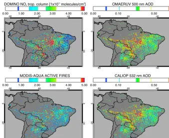
Figure 1. The 2006–2008 fire season (July–November) average DOMINO v2 NO2 tropospheric columns, OMAERUV 500 nm AOD,

MODIS-Aqua active fires, and CALIOP lv2 532 nm AOD. Pixels were selected and re-gridded to 0.25◦×0.25◦if all of the following conditions were met: (1) MODIS-Aqua detected an active fire with at least 80 % confidence, (2) the DOMINO v2 retrieval reported tropo-spheric column flag equal to zero, (3) and the OMAERUV retrieval reported algorithm quality flag equal to zero. CALIOP lv2 pixels were collocated with OMI pixels by averaging together all daytime CALIOP extinction vertical profiles within 0.5◦of the OMI pixel center. For the AOD calculation we selected aerosol layers where the cloud–aerosol discrimination (CAD) score was less than−20, the QC flag was equal to 0 or 1, and the extinction uncertainty was less than 99.9. The average active fire number represents the 2006–2008 average number of observed daily active fires in each grid cell during the fire season.

dicates that CALIOP AOD is higher than MODIS, but the two observations are roughly within the combined expected uncertainty (Winker et al., 2013).

2.6 Satellite data selection and OMI-CALIOP

colocation

As we are interested in retrievals affected by biomass burning emissions, we filtered the OMI observations within our South American domain (36◦S to 14◦N and 84◦W to 30◦W) for pixels where MODIS-Aqua (MYD14) reported an active fire between July and November (the South American burning season) in 2006–2008 (Fig. 1). DOMINO pixels were se-lected if the “tropospheric column flag” was equal to zero (indicating a reliable retrieval). OMAERUV pixels were se-lected if the “algorithm quality flag” was equal to zero, indi-cating cloud-screened (“most reliable”) retrievals.

We created a data set of OMI-CALIOP collocated pixels by averaging together all daytime CALIOP extinction verti-cal profiles within 0.5◦of the OMI pixel center. We selected aerosol layers where the CAD score was less than−20, QC

flag equal to 0 or 1, and the extinction uncertainty was less than 99.9 (this value indicates a failed retrieval).

In Fig. 1 we show DOMINO v2.0 NO2 tropospheric columns, MODIS-Aqua active fires, OMAERUV AOD, and CALIOP AOD averaged over the 2006–2008 fire seasons (July–November). Over the three fire seasons, there were in total 13 356 OMI-CALIOP collocated pixels. In general, the highest observed tropospheric NO2and AOD occur in cen-tral and western Brazil, eastern Bolivia, and Paraguay, loca-tions with the most active fires. The 3-year average AODs measured by CALIOP at 532 nm and OMAERUV at 500 nm generally follow the same spatial patterns. The Pearson cor-relation coefficient of the two gridded 3-year averages is 0.61 (N=5803). The OMAERUV AOD at 500 nm is on aver-age 30 % lower than the CALIOP AOD at 532 nm, reflecting the sub-pixel sampling of CALIOP, the spectral dependence of the AOD, and differences in vertical sensitivity and the aerosol models used in the two retrievals.

(7)

0.0 0.5 1.0 1.5 2.0 2.5 3.0 3.5 4.0 4.5 5.0

Aerosol Layer Height [km]

0.0 0.1 0.2 0.3 0.4 0.5

Probability

Mean = 1.50 km Std. Dev. = 0.62 km

CALIOP ALH

OMAERUV ALH

Figure 2. The probability distributions of the prescribed aerosol

layer height (ALH) in the OMAERUV retrieval, and the effective ALH (Eq. 7) derived from CALIOP 532 nm observed aerosol ex-tinction vertical profiles. The mean and standard deviation of the CALIOP effective ALH are 1.5 and 0.62 km, respectively.

of the OMAERUV-prescribed ALH and the CALIOP effec-tive ALH over South America for biomass burning aerosols. For pixels where OMAERUV assigns an ALH equal to zero, this corresponds to an aerosol vertical profile with a max-imum at the surface that decays exponentially with a 2 km scale height. In Fig. 2 this is depicted as an ALH equal to 1.88, which is the effective ALH for such a profile. The mean CALIOP effective ALH is 1.5 km, the same default value that is utilized for carbonaceous aerosols in the OMAERUV re-trieval. However, there is substantial variability in the daily observations, which show that 50 % of the observations have an ALH less than 1.5 km.

Figure 3 shows the average shape of the observed CALIOP aerosol extinction vertical profile and the collocated simu-lated TM4 NO2profile for three ranges of CALIOP effective ALH: less than 1 km, 1–2 km, and greater than 2 km. This plot was made by scaling all extinction vertical profiles to an AOD of 0.5 and tropospheric NO2profiles to a vertical col-umn equal to 1 before averaging by layer. In general, the bulk of the NO2is concentrated between the surface and roughly 2 km or 800 hPa, which is expected because we have selected pixels that contain active fires (i.e., a nearby surface source). When the effective ALH is less than 1 km, the aerosol and NO2tend to follow the same profile shape and are well mixed together. Both profiles peak at the surface, indicating a com-mon nearby surface source. When the effective ALH is 1– 2 km, aerosols are well mixed from the surface to 2 km, while the NO2continues to peak at the surface. This may be a re-sult of the shorter lifetime of NO2, underestimated buoyant plume rise in the model, or both. Figure 3 also shows that an effective ALH greater than 2 km corresponds to less aerosol extinction near the surface and an elevated extinction peak at 2–3.5 km, indicative of regional transport. The NO2

con-0.0 0.1 0.2 0.3 0.4 0.5 0.6

CALIOP Aerosol Extinction [km−1_]

0 1 2 3 4 5 6

Altitude [km]

CALIOP ALH < 1 km

0.0 0.1 0.2 0.3 0.4 0.5 0.6

1 km <= CALIOP ALH < 2 km

0.0 0.1 0.2 0.3 0.4 0.5 0.6

2 km < CALIOP ALH

0.00 0.05 0.10 0.15 0.20 0.25 0.30

NO2 Concentration [ppbv]

0 1 2 3 4 5 6

Altitude [km]

0.00 0.05 0.10 0.15 0.20 0.25 0.30

Figure 3. The shape of the observed CALIOP aerosol extinction

vertical profile and the collocated simulated TM4 NO2profile for

three ranges of CALIOP effective ALH: less than 1 km, 1–2 km, and greater than 2 km. This plot was made by scaling all extinction vertical profiles to an AOD of 0.5 and NO₂profiles to a tropospheric vertical column equal to 1 before averaging by layer. The red dots indicate the average in each layer, and the extent of the blue boxes represents the first and third quartiles in each layer.

centration in the model profile is somewhat enhanced above 2 km as well (compared to the other two NO2profiles), but the peak in NO2concentration remains at the surface, a con-sequence of the shorter lifetime of NO2.

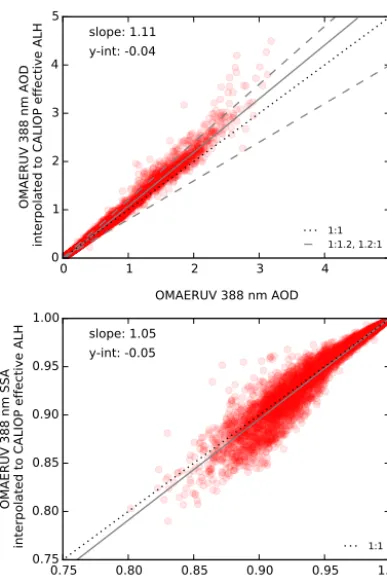
We replaced the OMAERUV-prescribed climatological ALH with observed CALIOP effective ALHs to obtain an estimate of the SSA and AOD that better reflects the daily variability of the aerosol vertical profile. To do this we in-terpolated the OMAERUV AOD and SSA given on the five altitude nodal points to the CALIOP ALH (Fig. 4). On average, the AOD interpolated to the effective ALH was 7 % higher than the AOD derived from the OMAERUV-prescribed ALH. There was on average no change in the SSA. Small increases in AOD are expected because although the OMAERUV assumed aerosol layer heights are generally consistent with the CALIOP observations, CALIOP obser-vations indicate that more profiles have enhanced aerosol ex-tinction closer to the surface (Fig. 2).

When collocated daily measurements are compared, the slope between CALIOP 532 nm AOD and OMAERUV 500 nm AOD is 0.65 and the correlation coefficient is 0.57. Figure 5 shows daily OMAERUV AOD measurements after adjusting for the CALIOP ALH. The slope increases to 0.70, comparable to the slope from the OMAERUV-AERONET evaluation discussed in Sect. 2.3, but there is no change in the correlation coefficient. For both choices of ALH, 68 % of the OMAERUV AOD observations were within 30 % of the CALIOP observations.

(8)

0 1 2 3 4 5 OMAERUV 388 nm AOD

0 1 2 3 4 5

OMAERUV 388 nm AOD

interpolated to CALIOP effective ALH

slope: 1.11 y-int: -0.04

1:1 1:1.2, 1.2:1

0.75 0.80 0.85 0.90 0.95 1.00

OMAERUV 388 nm SSA 0.75

0.80 0.85 0.90 0.95 1.00

OMAERUV 388 nm SSA

interpolated to CALIOP effective ALH

slope: 1.05 y-int: -0.05

1:1

Figure 4. The change in the OMAERUV 388 nm AOD and SSA

from replacing the standard retrieval prescribed aerosol layer height (ALH) with the CALIOP-observed effective ALH.

OMAERUV and CALIOP AOD, and that the AOD derived from CALIOP will likely not be as representative of the AOD for the DOMINO viewing scene as the OMAERUV AOD. The OMAERUV observations also provide the spectral in-formation needed to calculate the AOD at the DOMINO ref-erence wavelength. For these reasons, we scaled the CALIOP aerosol extinction vertical profiles to the OMAERUV AOD in our analysis. Thus, in our analysis CALIOP observations provide the aerosol vertical profile shape, but the AOD and SSA are based on OMI observations.

2.7 Calculation of altitude-resolved air mass factors

Altitude-resolved AMFs were computed with the DISAMAR (Determining Instrument Specifications and Analyzing Methods for Atmospheric Retrieval) radiative transfer model (de Haan, 2011). DISAMAR was designed to simulate re-trievals of properties of atmospheric trace gases, aerosols, clouds, and the ground surface for passive remote-sensing observations. Similar to the DAK radiative transfer model used to derive the DOMINO LUT, DISAMAR computes the reflectance and transmittance in the atmosphere using the po-larized doubling–adding method (de Haan et al., 1987). This method calculates the internal radiation field in the atmo-sphere for an arbitrary number of layers, in which Rayleigh

0.0 0.5 1.0 1.5 2.0 2.5 3.0 3.5

CALIOP 532 nm AOD

0.0

0.5 1.0 1.5 2.0 2.5 3.0 3.5

OMAERUV 500 nm AOD

interpolated to CALIOP effective ALH

Slope = 0.70 R = 0.58

1:1 1:1.3

0 10 20 30 40 50 60 70 80 90

Figure 5. Comparison of daily OMAERUV 500 nm AOD and

col-located CALIOP lv2 532 nm AOD for the 2006–2008 fire season (July–November) over South America. The gray solid line repre-sents the least squares fit through the origin. See Fig. 1 for the pixel and layer selection criteria.

scattering, gas absorption, and aerosol and cloud scattering and absorption can occur. A key difference between DAK and DISAMAR is that DISAMAR utilizes a separate altitude grid for the radiative transfer calculations that is independent of the grid used for specifying the atmospheric properties. This is important for simulating strong vertical gradients in the radiation field, e.g., near the top of clouds.

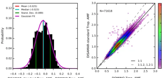
In Fig. 6, we show the comparison of NO2tropospheric AMFs from DOMINO v2.0 (based on the DAK-derived LUT) and DISAMAR for all retrievals with active fires in our South America domain (N=71 618). Identical to the DAK calculations for the DOMINO retrieval, in DISAMAR the altitude-resolved AMF was calculated at 439 nm and the sur-face reflectance was taken to be Lambertian and the atmo-sphere plane-parallel. However, in our analysis instead of in-terpolating the AMF from a LUT with fixed reference points for viewing geometry, albedo, and surface pressure for each OMI pixel we simulated the radiative transfer online using the exact values of surface albedo, effective cloud fraction and pressure, viewing geometry, and temperature, pressure, and NO2profiles from the DOMINO product.

(9)

0.4 0.3 0.2 0.1 0.0 0.1 0.2 0.3 0.4

DISAMAR-standard Trop. AMF - DOMINO Trop. AMF

0.00 0.02 0.04 0.06 0.08 0.10 0.12

Probability

Mean (-0.025) Median (-0.023) Stand. Dev. (0.089) Gaussian Fit

0.0 0.5 1.0 1.5 2.0 2.5 3.0

DOMINO Trop. AMF

0.0 0.5 1.0 1.5 2.0 2.5 3.0

DISAMAR-standard Trop. AMF

N=71618

1:1 1:1.2, 1.2:1

0 150 300 450 600 750 900 1050

Figure 6. The probability distribution of the differences in AMF retrieved by DISAMAR and DOMINO for all pixels in which

MODIS-Aqua reported an active fire between July and November in 2006–2008. The DOMINO tropospheric AMF data were filtered for tropospheric quality flag equal to zero and surface albedo less than 0.3.

0.8 0.6 0.4 0.2 0.0 0.2 0.4 0.6 0.8

DISAMAR-aerosol Trop. AMF - DISAMAR-standard Trop. AMF

0.00 0.01 0.02 0.03 0.04 0.05 0.06

Probability

Median (0.107)

0.0 0.5 1.0 1.5 2.0

DISAMAR-standard Trop. AMF

0.0 0.5 1.0 1.5 2.0

DISAMAR-aerosol Trop. AMF

N=13356

1:1 1:1.2, 1.2:1

0 20 40 60 80 100 120 140 160 180

Figure 7. Comparison between DISAMAR tropospheric AMFs calculated with the standard retrieval using parameters from DOMINO v2.0

(DISAMAR-standard), and DISAMAR tropospheric AMFs calculated with explicit aerosol effects (DISAMAR-aerosol). The AOD and SSA for these retrievals are determined by the OMAERUV retrieval, and aerosol extinction profiles were taken from the CALIOP lv2 retrieval.

larger as the standard deviation of the differences is 0.086 (8 %), putting an upper bound on this error of approximately 20 %. Henceforth, we will refer to the DISAMAR retrieval implementing the DOMINO configuration as DISAMAR-standard.

In order to model aerosol absorption and scattering ef-fects explicitly, we took SSA and AOD from OMAERUV retrievals, and aerosol extinction vertical profiles from co-located CALIOP observations. In the retrievals with explicit aerosol effects, for each pixel we used the DOMINO view-ing geometry, surface albedo, and temperature, pressure, and NO2vertical profiles, but excluded the DOMINO cloud pa-rameters, because we assume each OMAERUV scene is cloud free, as we only consider OMAERUV retrievals with algorithm quality flag equal to zero. Although we are only able to analyze ostensibly cloud-free pixels, the strength of this approach is that the AOD, SSA, and NO2slant columns and AMFs are derived from identical scenes.

We do not expect residual cloud contamination to signif-icantly affect our results because we limited our analysis to pixels where active fires are detected by MODIS-Aqua, and clear skies facilitate favorable conditions for open burning.

An additional check was made by comparing the CALIOP measured cloud+aerosol optical depth (CAD scores less than−20 and greater than 20) to the AOD. The increase in optical depth was negligible (< 0.1 %). After implementing the active fire filter, effective cloud radiance fractions (which arise due to the effects of aerosols on TOA reflectance in the O2–O2band) do not exceed 50 %, the threshold typically im-plemented when analyzing NO2tropospheric columns.

(10)

0.0 0.5 1.0 1.5 2.0 2.5

Altitude Resolved AMF

400 500 600 700 800 900 1000 Pressure [hPa]

DOMINO : 0.89 SSA = 1.00 AOD = 0.17

Cloud Radiance Fraction = 10% DISAMAR-STANDARD: 0.81 DISAMAR-CALIOP: 0.90

0 200 400 600 800 1000 1200

NO2 Concentrations [pptv]

400 500 600 700 800 900 1000

NO2 Profile

O2-O2 Cloud Top Pressure

CALIOP Effective Aerosol Layer Pressure

0.00 0.01 0.02 0.03 0.04 0.05 0.06 0.07532 nm Aerosol Extinction [km

−1]

CALIOP Aerosol Extinction

0.0 0.5 1.0 1.5 2.0 2.5

400 500 600 700 800 900 Pressure [hPa]

DOMINO : 1.25 SSA = 1.00 AOD = 0.38

0 50 100 150 200 250 300 350

400 500 600 700 800 900

NO2 Profile

0.00 0.02 0.04 0.06 0.08 0.10 0.12 0.14 0.16532 nm Aerosol Extinction [km

−1]

Figure 8. On the left are altitude-resolved AMFs from the

DISAMAR-standard and DISAMAR-aerosol calculations. The tro-pospheric AMF is given next to each label in the legend, and the DOMINO tropospheric AMF is given for reference. On the right are the NO2profiles from the TM4 simulations that are used in the

retrievals, along with the CALIOP lv2 aerosol extinction profiles utilized in the DISMAR-aerosol calculations. In all the plots, the O2–O2-retrieved effective cloud top pressure is shown as a

hori-zontal black line, and the CALIOP effective aerosol layer pressure is shown as a dashed horizontal gray line. For this figure we show the results for typical retrievals where the difference between the DISAMAR-standard and DISAMAR-aerosol tropospheric AMFs is less than±0.2.

3 Results: OMI NO2air mass factors with explicit

aerosol effects

In Fig. 7 we show the comparison of tropospheric AMFs calculated with the standard and DISAMAR-aerosol retrievals for all 13 356 OMI-CALIOP collocated pixels over South America. Tropospheric AMFs are on av-erage 11 % higher when OMAERUV and CALIOP aerosol characteristics (instead of effective O2–O2cloud parameters) are implemented in the retrieval. The asymmetrical probabil-ity distribution of the differences in AMF has a peak at 0.04. Approximately 66 % of the pixels differ by less than ±0.2 (18 %), within the 20 % estimated lower limit for the AMF uncertainty for polluted scenes (Boersma et al., 2004). The remaining roughly 34 % of the pixels lie in the positive tail of the probability distribution. In the following, we will an-alyze the retrieval conditions that generate small and large differences in the tropospheric AMF.

Figure 8 shows typical altitude-resolved AMFs, CALIOP aerosol extinction profiles, and simulated TM4 NO2profiles

0.0 0.5 1.0 1.5 2.0 2.5

400 500 600 700 800 900 Pressure [hPa]

DOMINO : 0.79 SSA = 1.00 AOD = 0.59

0 100 200 300 400 500 600 700

400 500 600 700 800 900

NO2 Profile

CALIOP Effective Aerosol Layer Pressure 0.0532 nm Aerosol Extinction [km0.1 0.2 0.3 0.4 0.5 0.6

−1]

0.0 0.5 1.0 1.5 2.0 2.5

400 500 600 700 800 900 Pressure [hPa]

DOMINO : 0.84 SSA = 0.92 AOD = 1.10

0 100 200 300 400

400 500 600 700 800 900

NO2 Profile

0.0 0.1 0.2 0.3 0.4 0.5 0.6 0.7 0.8 0.9532 nm Aerosol Extinction [km

−1]

Figure 9. On the left are altitude-resolved AMFs from the

DISAMAR-standard and DISAMAR-aerosol calculations. The tro-pospheric AMF is given next to each label in the legend, and the DOMINO tropospheric AMF is given for reference. On the right are the NO2 profiles from the TM4 simulations that are used in

the retrievals, along with the CALIOP lv2 aerosol extinction pro-files utilized in the DISMAR-aerosol calculations. In all the plots, the O2–O2-retrieved effective cloud top pressure is shown as a

hori-zontal black line, and the CALIOP effective aerosol layer pressure is shown as a dashed horizontal gray line. For this figure we show the results for two typical retrievals where the difference between the DISAMAR-standard and DISAMAR-aerosol tropospheric AMFs is greater than 0.2.

for two pixels where the difference in tropospheric AMF is less than±0.2 (i.e., when the implicit aerosol correction gen-erates tropospheric AMFs that agree reasonably well with AMF calculations that include observed aerosol parameters). Figure 9 shows the same data for two pixels where the dif-ference is greater than±0.2 (i.e., where the implicit aerosol correction fails).

(11)

-400 -300 -200 -100 0 100 200

O2-O2 CP - CALIOP ALP [hPa]

0.2 0.4 0.6 0.8 1.01.2 1.4 1.6 1.8 2.0 2.2 2.4 (a)

0.15 0.45 0.75 1.05 1.35 1.65 1.95 2.25 2.55 2.85

OMAERUV AOD 0.2

0.4 0.6 0.81.0 1.2 1.4 1.6 1.8 2.02.2 2.4 (b)

575 625 675 725 775 825 875 925 975

O2-O2 Effective Cloud Pressure [hPa]

0.2 0.4 0.6 0.8 1.01.2 1.4 1.6 1.8 2.0 2.2 2.4 (c)

2.0 6.0 10.0 14.0 18.0 22.0 26.0 30.0 34.0 38.0 42.0 46.0 50.0

O2-O2 Cloud Radiance Fraction [%]

0.2 0.4 0.6 0.81.0 1.2 1.4 1.6 1.8 2.02.2 2.4 (d)

2.6 8.2 14 19 27 27 3.1 41 30 15 6.2 3.4 2.4 1.5 0.6 0.3 0.07

6.9 8.0 8.8 9.6 10.0 12 19 18 7.2 8.3 7.3 8.9 10 12 10 9.1 7.7 7.0 6.3 6.1 5.1 2.1

DISAMAR-aerosol Trop. AMF / DISAMAR-standard Trop. AMF

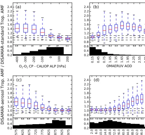
Figure 10. The ratio of the DISAMAR-aerosol tropospheric AMF

to the DISAMAR-standard tropospheric AMF with respect to

(a) the difference in the CALIOP effective aerosol layer

pres-sure (ALP) and the O2–O2 effective cloud top pressure, (b) the

OMAERUV AOD, (c) the O2–O2effective cloud top pressure, and

(d) the O2–O2cloud radiance fraction. The red lines represent the

mean for each bin. The extent of the blue boxes represents the first and third quartiles for each bin. Finally, the whiskers represent 3 standard deviations for each bin. The black boxes and numbers at the bottom of each plot are the fractions in percent of the total num-ber of pixels that fall in each bin. The dashed horizontal black lines are the 1.1, 1.0, and 0.9 horizontal grid lines.

575.00 625.00 675.00 725.00 775.00 825.00 875.00 925.00 975.00

O2-O2 CP [hPa]

400 300 200 100 0 100 200 300

O2

-O2

C

P

C

AL

IO

P A

LP

[h

Pa

]

Figure 11. The difference in the CALIOP effective aerosol layer

pressure (ALP) and the O2–O2effective cloud top pressure with

re-spect to the O2–O2effective cloud top pressure. The red lines

repre-sent the mean for each bin. The extent of the blue boxes reprerepre-sents the first and third quartiles for each bin. The whiskers represent 3 standard deviations for each bin.

gradually compared to the opaque cloud because generally aerosols are not concentrated in a single optically thick layer and aerosol scattering within the aerosol layer increases sen-sitivity to NO2.

Table 1. Ranges of parameters that are observed by OMI for which

less than 20 % biomass burning aerosol-related average error in the AMF can be expected.

Expected average Effective cloud Effective Aerosol AMF error radiance fraction cloud pressure optical depth

<20 % <30 % >800 hPa <0.6

Comparing Figs. 8 and 9, the factors that distinguish re-trievals with large differences from those with small differ-ences in tropospheric AMFs are lower effective cloud pres-sure, higher effective cloud fraction, and higher AOD. Also, in pixels where the effective cloud correction fails (Fig. 9), the O2–O2 effective cloud is typically higher than or at the top of the aerosol layer and the effective cloud shields a larger fraction of the atmosphere. Figure 9 also shows that because the AOD and effective cloud fraction are strongly correlated, the higher AOD in the pixels where the effec-tive cloud correction fails results in a larger weighting of the cloudy component of the tropospheric AMF, and a lower altitude-resolved AMF within the aerosol layer (Eq. 1).

In Fig. 10, we binned the differences in tropospheric AMF (DISAMAR-aerosol – DISAMAR-standard) for all 13 356 pixels considered according to the difference between the O2–O2 effective cloud pressure and the CALIOP effective aerosol layer pressure (ALP), the OMAERUV AOD, the O2– O2 effective cloud pressure, and the O2–O2 effective cloud radiance fraction. For the majority of the pixels (73 %), the O2–O2 effective cloud pressure and the CALIOP effective ALP were within 150 hPa. As the reduction in sensitivity to NO2occurs at approximately the same height in the two re-trievals, the implicit aerosol correction yields a tropospheric AMF that is on average within 20 % of the AMF calculated with explicit aerosol effects. In general, if the O2–O2 effec-tive cloud pressure is greater than 800 hPa (56 % of pixels), the difference in tropospheric AMF is on average less than ∼10 % (Fig. 10c) because the CALIOP effective ALP tends to be within 100 hPa (Fig. 11).

(12)

465 470 475 480 485 Wavelength [nm] 0.000

0.005 0.010 0.015 0.020 0.025

Differential Optical Thickness

(a)

850 hPa Aerosol Layer SSA=1.00 AOD=1.500 Sur. Alb.=0.040 900 hPa Lambertian Cloud Sur. Alb.=0.040 850 hPa 750 hPa 650 hPa

465 470 475 480 485

Wavelength [nm] 0.000

0.005 0.010 0.015 0.020 0.025

(b)

465 470 475 480 485

0.005 0.010 0.015 0.020 0.025

(c)

465 470 475 480 485

0.005 0.010 0.015 0.020 0.025

(d)

Figure 12. Simulations of differential optical thickness for an

aerosol layer centered at 850 hPa and extending for 300 hPa (solid red line). In each figure the differential optical thicknesses of Lam-bertian clouds with continuum reflectance equal to that of the aerosol layer simulation (i.e., equal cloud fraction) are shown for different cloud pressures (dashed lines).

The largest mean differences between the DISAMAR-aerosol and DISAMAR-standard retrieval occur for O2–O2 effective cloud pressures more than 150 hPa lower than the CALIOP effective ALP (approximately 24 % of the pix-els) (Fig. 10a), and for AODs greater than 0.6 (approxi-mately 30 % of the pixels) (Fig. 10b). These situations cor-respond with significantly stronger screening in the effec-tive cloud approach compared to AMF calculations based on observed aerosol parameters. The DISAMAR-aerosol tropo-spheric AMF for these low effective cloud pressure pixels is on average 30–50 % higher than the DISAMAR-standard AMF, but can be more than a factor of 2 higher for individual pixels.

Uncertainties in the observed aerosol parameters used in the DISAMAR-aerosol tropospheric AMF calculations can account for only part of the 30–50 % average difference be-tween the DISAMAR-standard and DISAMAR-aerosol cal-culations for high AODs (> 0.6) (see Appendix B); the up-per limit of the combined uncertainties in retrieved aerosol parameters is 25–30 %. The remaining difference between the DISAMAR-standard and DISAMAR-aerosol calcula-tions stems from a combination of misrepresenting the height of the aerosol layer (i.e., the DISAMAR-standard retrieval predicts decreased sensitivity to NO2 starting higher up in the atmosphere), overestimated shielding by the effective cloud (i.e., scattering by aerosols in the DISAMAR-aerosol retrieval predicts more sensitivity within the aerosol layer),

and a larger weighting of the cloudy component of the tropo-spheric AMF.

Several factors could lead to an O2–O2 effective cloud pressure that is smaller than the CALIOP effective aerosol layer pressure. First, internal retrieval assumptions for the surface pressure and temperature profile may lead to biases in retrieved effective cloud pressure (Maasakkers, 2013; Lin et al., 2014), but the biases are typically less than 100 hPa. Secondly, recall that the O2–O2slant column is the proxy for effective cloud pressure in the O2–O2cloud algorithm. This is based on the rationalization that a cloud has two main op-tical properties, transmission and reflection, and the O2–O2 slant column is a measure of the extent to which O2–O2 ab-sorption below the cloud has been shielded. Thus, the light-absorbing properties of aerosols are neglected in the O2–O2 retrieval Lambertian cloud model, and for strongly absorb-ing aerosols the reduced O2–O2slant column will be inter-preted as a smaller effective cloud pressure. For example, Figure 12a and b show simulations of the differential opti-cal thickness at 465–485 nm of an aerosol layer with AOD equal to 1.5 and SSA equal 1.00 and 0.90, respectively. The layer is centered at 850 hPa and extends for 300 hPa, a typical aerosol vertical profile (see Fig. 3), and the surface albedo is 0.04 in both simulations. In each figure the differential op-tical thicknesses of Lambertian clouds with continuum re-flectance equal to that of the aerosol layer simulation (i.e., equal cloud fraction) are shown for different cloud pressures. Figure 12a shows that the differential optical thickness of the aerosol layer with SSA equal to 1.00 corresponds to a Lambertian cloud between 850 and 900 hPa. When the SSA decreases to 0.90, the differential optical thickness for the aerosol layer is reduced and corresponds to a Lambertian cloud at 750 hPa (Fig. 12b).

Aerosol absorption would be enhanced if a strongly ab-sorbing layer were elevated above a more optically thick scat-tering layer or equivalently if the surface albedo increased. This is shown in Fig. 12c, where the surface albedo for the simulation of an aerosol layer with AOD equal to 1.5 and SSA equal to 0.90 is increased from 0.04 to 0.07. The 477 nm differential optical thickness now corresponds to a Lamber-tian cloud at 650 hPa. Figure 13 shows the comparison of sur-face albedo and the difference between the observed effective cloud pressure and the observed effective aerosol layer pres-sure. The figure indeed indicates that negative differences be-tween observed effective cloud pressure and observed effec-tive aerosol layer pressure are associated with larger surface albedos, particularly when the AOD exceeds 0.7.

(13)

0.01 0.03 0.05 0.07

440 nm Lambertian Equivalent Surface Reflectance 700

600 500 400 300 200 1000 100 200 300 400

O2

-O2

C

AL

IO

P A

LP

[h

Pa

]

388 nm AOD <= 0.70

0.01 0.03 0.05 0.07

440 nm Lambertian Equivalent Surface Reflectance 700

600 500 400 300 200 1000 100 200 300 400

O2

-O2

C

AL

IO

P A

LP

[h

Pa

]

388 nm AOD > 0.70

Figure 13. Comparison of the surface albedo utilized in the O2–

O₂retrieval with the difference between the O₂–O₂effective cloud pressure and the CALIOP-observed effective aerosol layer pressure.

contribution to the O2–O2slant column would increase. The observed slant column would therefore be interpreted as a smaller effective cloud pressure.

Aerosol absorption also significantly affects the retrieved O2–O2effective cloud fraction. Figure 14 shows that there is a strong correlation between the observed AOD and the ob-served effective cloud fraction. However, the slope of the lin-ear fit between AOD and cloud fraction decreases with SSA. Cloud fractions for scattering aerosols (SSA > 0.95) are ap-proximately 1.5–2 times larger than cloud fractions for ab-sorbing aerosols. Thus, although scattering aerosols lead to larger retrieved effective cloud pressures, in the AMF calcu-lation a larger weighting of the cloudy component of the tro-pospheric AMF will enhance shielding. Meanwhile, for ab-sorbing aerosols, enhanced shielding in the AMF calculation due to smaller retrieved effective cloud pressures is offset by smaller effective cloud fractions. This highlights the compen-sating mechanisms at play behind the implicit aerosol correc-tion in the current DOMINO NO2retrieval for scenes with high aerosol optical depth and indicates the need for further investigation of the response of the O2–O2 effective cloud retrieval to aerosol contamination.

4 Discussion and conclusions

In this paper we analyzed the properties of the implicit aerosol correction in the DOMINO tropospheric NO2 re-trieval and presented an observation-based aerosol correction scheme using collocated OMI and CALIOP observations. We utilized 3 years of observations over South America, fo-cusing on clear-sky pixels affected by biomass burning emis-sions. When all pixels were considered, tropospheric AMFs calculated with observed aerosol parameters were on aver-age only 10 % higher than AMFs calculated with effective cloud parameters. Thus, errors in the implicit aerosol cor-rection will be minimized in regional and seasonal averages of NO2tropospheric columns. However, for individual pix-els, when aerosol scattering and absorption is considered the

0.0

0.5

1.0

1.5

2.0

2.5

3.0

3.5 OMAERUV 388 nm AOD

0.00

0.02

0.04

0.06

0.08

0.10

0.12

0.14

0.16

0.18 O

2

-O

2

E

ffe

cti

ve

C

lou

d

Fr

ac

tio

n

CF = 0.13*AOD R = 0.87

CF = 0.08*AOD + 0.01 R = 0.93

CF = 0.05*AOD + 0.02 R = 0.92

CF = 0.05*AOD + 0.01 R = 0.87 0.95 < SSA 0.90 < SSA <= 0.95 0.85 < SSA <= 0.90 SSA <= 0.85

Figure 14. Comparison of the OMAERUV-retrieved 388 nm AOD

and observed effective cloud fraction binned by the OMAERUV-retrieved SSA.

tropospheric AMF can increase by as much as a factor of 2 compared to the implicit aerosol correction approach.

From our analysis we identified the ranges of retrieved O2–O2effective cloud parameters where it is possible to dis-tinguish pixels that have minimal errors from aerosol effects on the tropospheric AMF, as both the effective cloud frac-tions and the effective cloud pressures contain information about the aerosol concentration and vertical distribution. By filtering for effective cloud radiance fraction less than 0.3, or effective cloud pressure greater than 800 hPa, the difference between tropospheric AMFs based on implicit and explicit aerosol parameters is on average 6 % and 3 %, respectively. These parameters fit the majority of the pixels considered in our study; 70 % had cloud radiance fraction below 30 %, and 50 % had effective cloud pressure greater than 800 hPa. We recommend using these ranges as a practical way to mini-mize aerosol-related errors in version 2.0 of DOMINO NO2 tropospheric columns when the presence of biomass burn-ing aerosol emissions is expected. For validation experiments where aerosol interferences are likely, it may be possible to separate aerosol interference errors in the NO2tropospheric column from other retrieval algorithm errors by comparing observations under different cloud radiance fraction thresh-olds.

(14)

AMFs were on average 20–40 % larger than the tropospheric AMFs derived using effective cloud parameters. These sit-uations correspond with overestimated shielding in the im-plicit aerosol correction approach because the assumption of an opaque cloud underestimates the altitude-resolved AMF below the effective cloud.

Simulations of O2–O2 differential optical thickness at 465–490 nm (the spectral window of the effective cloud re-trieval) show that neglecting aerosol absorption in the Lam-bertian cloud model leads to lower retrieved effective cloud pressures as reduced O2–O2slant columns will be interpreted as a lower effective cloud pressures. This error was enhanced by higher surface albedos. Radiative transfer simulations of a typical aerosol layer showed that even lower effective cloud pressures could be retrieved if there is a high bias in the ob-served surface albedo monthly climatology. Sub-pixel cloud or aerosol contamination could lead to surface albedo errors. Particularly for pixels where active biomass burning is occur-ring, short-term darkening of the surface may not be captured in the monthly climatology because of the relatively coarse resolution of the data set. Furthermore, outside of African sa-vannas, most ecosystems do not burn every year, and after a burn the surface albedo recovers to pre-fire levels within 1–2 years (Gatebe et al., 2014). Thus, a higher spatial and tem-poral resolution surface albedo data set may be necessary to retrieve reliable effective cloud parameters for scenes with active biomass burning. In general, further research is needed to better interpret the retrieved O2–O2effective cloud param-eters in the presence of aerosols.

Above an effective cloud fraction of 0.3 or an AOD of 0.60, tropospheric AMFs calculated with observed aerosol parameters were on average 30–50 % larger than the tro-pospheric AMFs derived using effective cloud parameters. These differences cannot be accounted for by the uncertain-ties in the retrieved aerosol parameters. This implies that for large fires or smoldering fires that release significant amounts of aerosols, the DOMINO NO2 tropospheric columns may be significantly overestimated. In general, this has implica-tions for the estimation of emissions from satellite NO2 tro-pospheric column measurements for any source that is corre-lated with high aerosol concentrations and suggests that cur-rent top-down emissions estimates could be overestimated.

In our analysis we compared AMFs from the DOMINO retrieval calculated by interpolating a look-up table with radiative transfer calculations from DISAMAR; the mean and standard deviation of the difference was −0.6±8 %. We also presented the first comparison of collocated AOD from the OMI near UV aerosol retrieval (OMAERUV) and CALIOP level 2 aerosol extinction vertical profile observa-tions. We found good spatial correlation in the 3-year average (R=0.6), and 68 % of the daily OMAERUV AOD tions were within 30 % of the collocated CALIOP observa-tions.

Our analysis holds promise for a strategy to include the ef-fect of aerosols on tropospheric AMF calculations for clear-sky pixels based on globally available satellite observations. Although, on average, the differences in tropospheric AMFs calculated with effective cloud parameters versus observed aerosol parameters are small, tropospheric AMFs can differ by more than a factor of 2.

In the presence of actual clouds, the effect of aerosols on the tropospheric AMF may be offset or enhanced depending on the amount and height of the clouds (Lin et al., 2014). As aerosol optical depth from OMI is not observable in the pres-ence of clouds, further work is needed to exploit data from high spatial resolution aerosol sensors that can resolve scene heterogeneity, as well as global atmospheric simulations of aerosols.

(15)

Appendix A:

0.0 0.5 1.0 1.5 2.0 2.5 3.0 3.5

OMAERUV AOD 0.75

0.80 0.85 0.90 0.95 1.00 1.05 1.10 1.15

DISAMAR-aerosol(g=0.6) / DISAMAR-aerosol

AMF Sensitivity to Asymmetry Parameter (g)

0 15 30 45 60 75 90 105 120 135

Figure A1. The change in the calculated tropospheric AMF as a

result of a decrease from 0.7 to 0.6 in the aerosol asymmetry pa-rameter (g) used in the DISAMAR radiative transfer model.

In the OMAERUV retrieval pixels are labeled as cloud free if one of the following three conditions occurs: (1) car-bonaceous aerosol has been identified and the measured re-flectivity at 388 nm is less than 0.16, (2) the difference be-tween the measured scene reflectivity and the assumed sur-face albedo (1R)is less than or equal to 0.07, or (3) car-bonaceous aerosol has been identified and 1R is less than or equal to 0.08 and the UV aerosol index (UVAI) is greater than or equal to 0.3.

The UVAI is a measure of the deviation of the observed UV spectral contrast from a pure Rayleigh scattering atmo-sphere. UVAI will be negative for scattering aerosols (Pen-ning de Vries et al., 2009), positive for absorbing aerosols, and will increase with the height, the optical depth and the single scattering co-albedo of the absorbing aerosol layer (de Graaf, 2005; Torres et al., 1998).

0.0 0.5 1.0 1.5 2.0 2.5 3.0 3.5 OMAERUV AOD

0.75 0.80 0.85 0.90 0.95 1.00 1.05 1.10 1.15

DISAMAR-aerosol(AOD-30% or 0.1) / DISAMAR-aerosol

AMF Sensitivity to AOD

ALH <= 2 km 2 km < ALH <= 3 km 3 km < ALH

0.0 0.5 1.0 1.5 2.0 2.5 3.0 3.5 OMAERUV AOD 0.75

0.80 0.85 0.90 0.95 1.00 1.05 1.10

1.15 AMF Sensitivity to AOD

0 15 30 45 60 75 90 105 120 135

result of a 30 % or 0.1 decrease (whichever is larger) in the AOD used in the DISAMAR radiative transfer model.

0.0 0.5 1.0 1.5 2.0 2.5 3.0 3.5

OMAERUV AOD 0.75

0.80 0.85 0.90 0.95 1.00 1.05 1.10 1.15

DISAMAR-aerosol(SSA-0.05) / DISAMAR-aerosol

AMF Sensitivity to SSA

0 25 50 75 100 125 150 175 200 225

(16)

Appendix B:

The following sensitivity analysis shows how the uncer-tainties in the observed aerosol parameters used in the DISAMAR-aerosol tropospheric AMF calculations can ac-count for only part of the 30–50 % average difference be-tween the DISAMAR-standard and DISAMAR-aerosol cal-culations for high AODs (> 0.6). Figures A1–A3 show the change in the DISAMAR-aerosol AMF when (a) the SSA is reduced by 0.05, the threshold for agreement for 75 % of OMAERUV SSA retrievals with AERONET observa-tions, (b) the AOD is reduced by 30 % or 0.1 (whichever is greater), the estimated uncertainty of the OMAERUV AOD, and (c) the asymmetry parameter is reduced from 0.7 to 0.6, the approximate lower limit for the absorbing aerosol models used in the OMAERUV retrieval. AERONET observations during the dry season in South America show that the av-erage and standard deviation of the asymmetry parameter at 440 nm is 0.68±0.02, with a range of 0.6 to 0.75 (Rosáraio et al., 2011; Sena et al., 2013).

A 0.1 decrease in the asymmetry parameter resulted in an approximately 5 % (maximum 10 %) increase in AMF that is weakly correlated with AOD above AOD equal to ∼0.5 (Fig. A1). At low optical thickness, the increase in AMF in-creases with AOD, consistent with an increase in the albedo effect from aerosols. The effect of reducing the AOD in the tropospheric AMF calculation depends on the effective ALH (Fig. A2), which to first order determines whether the aerosols shield NO2below, or enhance the light path and re-flectance from within an aerosol–NO2mixed layer. For ele-vated aerosol layers (ALH > 3 km), the decrease in AOD re-sulted in a small decrease (< 5 %) or an increase (< 5 %) in AMF, consistent with a partial shielding aerosol effect. Re-gardless of ALH, when the AOD exceeds 2, aerosols are pre-dominantly shielding, and a decrease in the AOD results in a 0–10 % increase in AMF. When the aerosol extinction profile has an effective ALH less than 2 km, a decrease in the AOD results in at most a 20 % decrease in AMF, but on average a 5–10 % decrease, indicating a predominantly albedo aerosol affect.

(17)

The Supplement related to this article is available online at doi:10.5194/amt-8-3831-2015-supplement.

Acknowledgements. The authors thank the CALIOP project for

producing and making available the data sets used in this analysis. We also thank the AERONET project and the principal investi-gators of the sites used in this work, and Maarten Sneep for the development of py-DISAMAR. Patricia Castellanos acknowledges Guido van der Werf and funding from the Netherlands Space Office (NSO), project ALW-GO-AO/10-01. Folkert Boersma acknowledges receiving funding for this research from NWO Vidi Grant 864.09.001 and from the European Community’s Seventh Framework Programme under grant agreement no. 607405 (QA4ECV).

Edited by: M. Van Roozendael

References

Acarreta, J. R., de Haan, J. F., and Stammes, P.: Cloud pressure re-trieval using the O2–O2absorption band at 477 nm, J. Geophys.

Res., 109, D05204, doi:10.1029/2003JD003915, 2004.

Ahn, C., Torres, O., and Jethva, H.: Assessment of OMI near UV aerosol optical depth over land, J. Geophys. Res. Atmos., 119, 2457–2473, 2014.

Beirle, S., Boersma, K. F., Platt, U., Lawrence, M. G., and Wagner, T.: Megacity Emissions and Lifetimes of Nitro-gen Oxides Probed from Space, Science, 333, 1737–1739, doi:10.1126/science.1207824, 2011.

Boersma, K. F., Eskes, H. J., and Brinksma, E. J.: Error analysis for tropospheric NO2retrieval from space, J. Geophys. Res., 109,

D04311, doi:10.1029/2003JD003962, 2004.

Boersma, K. F., Eskes, H. J., Dirksen, R. J., van der A, R. J., Veefkind, J. P., Stammes, P., Huijnen, V., Kleipool, Q. L., Sneep, M., Claas, J., Leitão, J., Richter, A., Zhou, Y., and Brun-ner, D.: An improved tropospheric NO2column retrieval

algo-rithm for the Ozone Monitoring Instrument, Atmos. Meas. Tech., 4, 1905–1928, doi:10.5194/amt-4-1905-2011, 2011.

Braak, R.: Row Anomaly Flagging Rules Lookup Table, KNMI, De Bilt, 2010.

Bucsela, E. J., Pickering, K. E., Huntemann, T. L., Cohen, R. C., Perring, A., Gleason, J. F., Blakeslee, R. J., Albrecht, R. I., Holz-worth, R., Cipriani, J. P., Vargas-Navarro, D., Mora-Segura, I., Pacheco-Hernández, A., and Laporte-Molina, S.: Lightning-generated NOxseen by the Ozone Monitoring Instrument

dur-ing NASA’s Tropical Composition, Cloud and Climate Cou-pling Experiment (TC 4), J. Geophys. Res., 115, D00J10, doi:10.1029/2009JD013118, 2010.

Castellanos, P. and Boersma, K. F.: Reductions in nitrogen oxides over Europe driven by environmental policy and economic reces-sion, Sci. Rep., 2, 265, doi:10.1038/srep00265, 2012.

Castellanos, P., Boersma, K. F., and van der Werf, G. R.: Satel-lite observations indicate substantial spatiotemporal variability in biomass burning NOx emission factors for South America,

Atmos. Chem. Phys., 14, 3929–3943, doi:10.5194/acp-14-3929-2014, 2014.

Caudill, T. R., Flittner, D. E., Herman, B. M., Torres, O., and McPeters, R. D.: Evaluation of the pseudo-spherical approxima-tion for backscattered ultraviolet radiances and ozone retrieval, J. Geophys. Res., 102, 3881, doi:10.1029/96JD03266, 1997. de Graaf, M.: Absorbing Aerosol Index: sensitivity analysis,

appli-cation to GOME and comparison with TOMS, J. Geophys. Res., 110, D01201, doi:10.1029/2004JD005178, 2005.

de Haan, J. F.: DISAMAR Algorithm description and background information, Royal Netherlands Meteoroligical Institute, De Bilt, the Netherlands, 2011.

de Haan, J. F., Bosma, P. B., and Hovenier, J. W.: The adding method for multiple scattering calculations of polarized light, Astron. Astrophys., 183, 371–391, 1987.

de Ruyter de Wildt, M., Eskes, H., and Boersma, K. F.: The global economic cycle and satellite-derived NO2 trends

over shipping lanes, Geophys. Res. Lett., 39, L01802, doi:10.1029/2011GL049541, 2012.

De Smedt, I., Van Roozendael, M., Stavrakou, T., Müller, J.-F., Lerot, C., Theys, N., Valks, P., Hao, N., and van der A, R.: Im-proved retrieval of global tropospheric formaldehyde columns from GOME-2/MetOp-A addressing noise reduction and instru-mental degradation issues, Atmos. Meas. Tech., 5, 2933–2949, doi:10.5194/amt-5-2933-2012, 2012.

Dirksen, R. J., Boersma, K. F., Eskes, H. J., Ionov, D. V., Buc-sela, E. J., Levelt, P. F., and Kelder, H. M.: Evaluation of strato-spheric NO₂retrieved from the Ozone Monitoring Instrument: intercomparison, diurnal cycle, and trending, J. Geophys. Res., 116, D08305, doi:10.1029/2010JD014943, 2011.

Dubovik, O., Holben, B., Eck, T. F., Smirnov, A., Kaufman, Y. J., King, M. D., Tanré, D., and Slutsker, I.: Variability of absorption and optical properties of key aerosol types observed in world-wide locations, J. Atmos. Sci., 59, 590–608, 2002.

Eskes, H. J. and Boersma, K. F.: Averaging kernels for DOAS total-column satellite retrievals, Atmos. Chem. Phys., 3, 1285–1291, doi:10.5194/acp-3-1285-2003, 2003.

Gatebe, C. K., Ichoku, C. M., Poudyal, R., Roman, M. O., and Wilcox, E.: Surface albedo darkening from wildfires in northern sub-Saharan Africa, Environ. Res. Lett., 9, 065003, doi:10.1088/1748-9326/9/6/065003, 2014.

Giglio, L., Randerson, J. T., van der Werf, G. R., Kasibhatla, P. S., Collatz, G. J., Morton, D. C., and DeFries, R. S.: Assess-ing variability and long-term trends in burned area by mergAssess-ing multiple satellite fire products, Biogeosciences, 7, 1171–1186, doi:10.5194/bg-7-1171-2010, 2010.

Holben, B. N., Eck, T. F., Slutsker, I., Tanré, D., Buis, J. P., Set-zer, A., Vermote, E., Reagan, J. A., Kaufman, Y. J., Nakajima, T., Lavenu, F., Jankowiak, I., and Smirnov, A.: AERONET – a fed-erated instrument network and data archive for aerosol charac-terization, Remote Sens. Environ., 66, 1–16, doi:10.1016/S0034-4257(98)00031-5, 1998.

Irie, H., Boersma, K. F., Kanaya, Y., Takashima, H., Pan, X., and Wang, Z. F.: Quantitative bias estimates for tropospheric NO2

columns retrieved from SCIAMACHY, OMI, and GOME-2 us-ing a common standard for East Asia, Atmos. Meas. Tech., 5, 2403–2411, doi:10.5194/amt-5-2403-2012, 2012.

Jaeglé, L., Steinberger, L., Martin, R. V., and Chance, K.: Global partitioning of NOxsources using satellite observations: relative