www.atmos-meas-tech.net/9/2425/2016/ doi:10.5194/amt-9-2425-2016
© Author(s) 2016. CC Attribution 3.0 License.
Retrieval algorithm for rainfall mapping from microwave links in a
cellular communication network
Aart Overeem1,2, Hidde Leijnse2, and Remko Uijlenhoet1
1Hydrology and Quantitative Water Management Group, Wageningen University, P.O. Box 47, 6700 AA, Wageningen, the Netherlands
2Royal Netherlands Meteorological Institute (KNMI), P.O. Box 201, 3730 AE, De Bilt, the Netherlands Correspondence to:Aart Overeem ([email protected])
Received: 18 July 2015 – Published in Atmos. Meas. Tech. Discuss.: 7 August 2015 Revised: 14 April 2016 – Accepted: 4 May 2016 – Published: 1 June 2016
Abstract.Microwave links in commercial cellular communi-cation networks hold a promise for areal rainfall monitoring and could complement rainfall estimates from ground-based weather radars, rain gauges, and satellites. It has been shown that country-wide (≈35 500 km2) 15 min rainfall maps can be derived from the signal attenuations of approximately 2400 microwave links in such a network. Here we give a detailed description of the employed rainfall retrieval algo-rithm. Moreover, the documented, modular, and user-friendly code (a package in the scripting language “R”) is made available, including a 2-day data set of approximately 2600 commercial microwave links from the Netherlands. The pur-pose of this paper is to promote rainfall mapping utilising microwave links from cellular communication networks as an alternative or complementary means for continental-scale rainfall monitoring.
1 Introduction
Accurate rainfall observations with high spatial and tempo-ral resolution are needed for hydrological applications, agri-culture, meteorology, weather forecasting, and climate mon-itoring. However, there is a lack of accurate rainfall infor-mation for the majority of the land surface of the earth, no-tably from ground-based weather radars (Heistermann et al., 2013). Moreover, the number of reporting rain gauges is dra-matically declining in Europe, South America, and Africa. Lorenz and Kunstmann (2012) report a decline of approx-imately 50 % in the period 1989–2006 for GPCC, version 5.0. Satellites are often the only source of rainfall
informa-tion. Despite their increasing coverage and spatio-temporal resolution, measurement errors and sampling uncertainties limit the stand-alone applicability of satellite rainfall prod-ucts (e.g. Sorooshian et al., 2000; Joyce et al., 2004; Roe-beling and Holleman, 2009; Kidd and Huffman, 2011; Hou et al., 2014). This calls for alternative and complementary sources of rainfall information. Since 2006 various studies have shown that microwave links from operational cellular communication networks may be used for rainfall monitor-ing for various networks and climates (e.g. Messer et al., 2006; Leijnse et al., 2007a; Zinevich et al., 2009; Overeem et al., 2011, 2013; Chwala et al., 2012; Rayitsfeld et al., 2012; Bianchi et al., 2013; Doumounia et al., 2014). The ability to observe other types of precipitation, such as snow, is limited however.
0 50
N
km North Sea
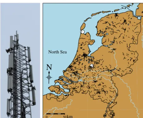
Figure 1.Left: illustration of a telephone tower. The electromag-netic signals transmitted from the directional antenna of one cellular communication tower to another are attenuated by rainfall. Right: map of the Netherlands with locations of the employed link paths (1527) from the cellular communication network for 9 September, 16:00 UTC–11 September, 08:00 UTC (2011). These were part of one network of one of the three providers in the Netherlands. The white circles show the locations of the two weather radars operated by the Royal Netherlands Meteorological Institute (KNMI).
over the path of a link. Rainfall estimates from networks of individual links could in turn potentially be employed to cre-ate near real-time rainfall maps. This is particularly interest-ing for (developinterest-ing) countries where few surface rainfall ob-servations are available. For instance, (Gosset et al., 2016), who report on a Rain Cell Africa workshop held in Burk-ina Faso in March 2015, clearly demonstrate the relevance and interest to accelerate the uptake of this new measure-ment technique on the African continent. Despite the sym-pathy from scientists and representatives of meteorological services and telecommunication companies, to date no user-friendly computer code for microwave link data processing and rainfall mapping has been made publicly available. That is the motivation of this paper.
Based on a 12-day data set Overeem et al. (2013) have shown that country-wide (≈35 500 km2) 15 min rainfall maps can be derived from received signal powers of mi-crowave links in a cellular communication network. Hence, further upscaling this novel source of rainfall information is the logical next step toward continental-scale rainfall moni-toring. The underlying rainfall retrieval algorithm is briefly described in Overeem et al. (2013) and largely based on Overeem et al. (2011). The purpose of this paper is to provide a detailed description of the algorithm employed by Overeem et al. (2013) and the corresponding computer code, which is needed for a successful implementation by potential users. Moreover, sensitivity analyses are performed with respect to
two threshold values of the wet–dry classification method and the outlier filter threshold value. Finally, the transferabil-ity of the code to other networks and climates is extensively discussed.
The code is freely provided as R package “RAINLINK” on GitHub1. It contains a working example to compute link-based 15 min rainfall maps for the entire surface area of the Netherlands for 40 h from real microwave link data as used in Overeem et al. (2013). This is a working example using actual data from an extensive network of commercial mi-crowave links, for the first time in the scientific literature, which will allow users to test their own algorithms and com-pare their results with ours. Note that link data are utilised in a stand-alone fashion to obtain rainfall maps; i.e. data from rain gauges, weather radars, or satellites are not combined with the link data.
The basic theory of rainfall estimation employing mi-crowave links has already been described, e.g. in Messer et al. (2006), Leijnse et al. (2007a), and Overeem et al. (2011). The core of the rainfall retrieval algorithm consists of the (path-averaged) rainfall intensityR (mm h−1) being estimated from microwave (path-averaged) specific attenua-tionk(dB km−1) using a power-lawR–krelation (Atlas and Ulbrich, 1977; Olsen et al., 1978):
R=akb. (1)
Coefficientsa(mm h−1dB−bkmb) and exponentsb(−) de-pend mainly on link frequency. The rainfall retrieval algo-rithm consists of the following steps: (1) preprocessing of link data; (2) wet–dry classification; (3) reference signal de-termination; (4) removal of outliers due to malfunctioning links; (5) correction of received signal powers; and (6) com-putation of mean path-averaged rainfall intensities. Below at-tention is given to the main retrieval issues associated with link-based rainfall estimation.
Received signal powers occasionally decrease during non-rainy periods, resulting in non-zero rainfall estimates, e.g. caused by reflection of the beam or dew formation on the antennas (see Upton et al. (2005) for an overview). A reli-able classification of wet and dry periods is needed to prevent this rainfall overestimation. Different classification methods have been proposed, some of which can be applied to re-ceived powers or signal attenuations when they are sampled at very high frequencies (often for research purposes), e.g. every 6 or 30 s (Schleiss and Berne, 2010) or even at 20 Hz. For instance, Chwala et al. (2012) present a spectral time se-ries analysis, and Wang et al. (2012) Markov switching mod-els. Here the so-called “nearby link approach” is employed (Overeem et al., 2011, 2013, termed “link approach” in these papers), which was derived for application to minimum re-ceived powers over a time interval (15 min in Overeem et al., 2011, 2013). A common operational sampling strategy for commercial microwave links is to obtain a minimum and
maximum received power per 15 min interval (Messer et al., 2006; Overeem et al., 2011, 2013). Hence, methods designed for frequently sampled attenuation data cannot be applied to data from such operational networks. However, the nearby link approach cannot be applied if spatial link densities are too low. Messer and Sendik (2015) provide more informa-tion on different methods of wet–dry classificainforma-tion and ref-erence signal determination. Sometimes powers are sampled every second (Doumounia et al., 2014), every minute (Ray-itsfeld et al., 2012), or only once or twice every 15 min (Lei-jnse et al., 2007a). Other approaches to identify rainy and non-rainy spells make use of auxiliary sources but are not considered in this paper. For instance, radar data have been utilised in the “radar approach” (Overeem et al., 2011), and geostationary satellite data in the “satellite approach” (Van het Schip et al., 2016). An advantage of the nearby link ap-proach is that it solely employs link data; i.e. it does not de-pend on auxiliary data.
Attenuation due to wet antennas gives rise to overestima-tion of rainfall and needs to be compensated for (Kharadly and Ross, 2001; Minda and Nakamura, 2005; Leijnse et al., 2007a, b, 2008; Schleiss et al., 2013). The sampling strategy is also an important error source, e.g. one sample every 15 min leads to large deviations due to unresolved rainfall vari-ability (Leijnse et al., 2008).
This paper is organised as follows. First a description of the required microwave link data is given. Next, the rain-fall retrieval algorithm and the interpolation methodology are described. The results section illustrates the different steps of the rainfall retrieval algorithm including rainfall mapping. Also sensitivity analyses of parameters of the algorithm are provided, as well as a comparison between the performance of two interpolation methods. Next, the algorithm and its ap-plicability to other networks and regions are discussed. Fi-nally, conclusions are provided.
2 Data
2.1 Microwave link data: characteristics and preparations
In order to compute path-averaged rainfall intensities, re-ceived signal powers were obtained from Nokia microwave links in one of the national cellular communication networks in the Netherlands, operated by T-Mobile NL. The minimum and maximum received powers over 15 min intervals were provided, based on 10 Hz sampling. The transmitted power was almost constant. Here the data have a resolution of 1 dB, and the majority of these Nokia links used vertically po-larised signals. The data format required by the code is given in Appendix A.
Data from the working example were obtained from 9 September, 08:00 UTC, to 11 September, 08:00 UTC (2011), to estimate rain (Overeem et al., 2016a). Figure 1 shows the locations of the links which can be used to estimate
rain-fall (on average 2473 links and 1527 link paths over all 160 time intervals of 15 min). Data from another day are used to illustrate the rainfall retrieval algorithm, but these data are not released with this paper. In addition, a 12-day validation data set, which includes the data from the working exam-ple, is used for sensitivity analyses of parameters of the rain-fall retrieval algorithm. This data set is from June, August, and September 2011. Overeem et al. (2013) and Rios Gaona et al. (2015) provide more information on the characteristics of microwave links from this 12-day data set. All link data are from an independent validation data set; i.e. they have not been used to calibrate the rainfall retrieval algorithm. 2.2 Gauge-adjusted radar rainfall depths
Overeem et al. (2013) use a gauge-adjusted radar data set with a spatial resolution of approximately 0.9 km2and a tem-poral resolution of 5 min to calibrate the microwave link rain-fall retrieval algorithm. Here this radar data set, from another period than the calibration period, is utilised to validate link-based rainfall maps. More information on the derivation of this data set can be found in Overeem et al. (2009a, b, 2011). The data set is freely available at the climate4impact portal (Overeem et al., 2016b).
3 Methodology
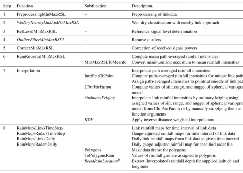
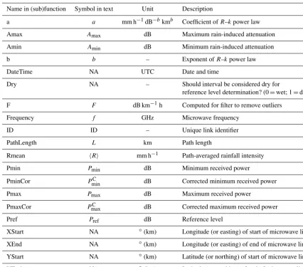
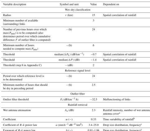
This section describes the entire processing chain from re-ceived signal powers to rainfall maps. The code is provided via GitHub as the R2 package called “RAINLINK” (ver-sion 1.11)3, which is distributed under the terms of GNU General Public License version 3 or later. Table 1 gives an overview of the (sub)functions needed for rainfall retrieval and mapping. Table 2 provides an overview of variables used in (sub)functions in the rainfall retrieval algorithm. Table 3 shows the parameters used in the rainfall retrieval algorithm and their default values. First, preprocessing of link data is performed (Appendix B).
3.1 Classification of wet and dry periods: the nearby link approach
In order to define wet and dry periods, it is assumed that rain is correlated in space and hence that several links in a given area should experience a joint decrease in received signal level in the case of rain. A time interval is labelled as wet if at least half of the links in the vicinity (default radius is 15 km, but this can be modified to better match other time intervals) of the selected link experience such a decrease. A detailed description of this classification algorithm can be found in Appendix C.
2http://www.r-project.org/
Table 1.Overview of functions needed for processing link data from received signal powers to rainfall maps. Italicised (sub)functions are optional. A choice has to be made between bold subfunctions. The script “Run.R” can be employed to determine which (sub)functions are being applied.
Step Function Subfunction Description
1 PreprocessingMinMaxRSL – Preprocessing of linkdata
2 WetDryNearbyLinkApMinMaxRSL Wet–dry classification with nearby link approach
3 RefLevelMinMaxRSL – Reference signal level determination
4 OutlierFilterMinMaxRSLa – Remove outliers
5 CorrectMinMaxRSL Correction of received signal powers
6 RainRetrievalMinMaxRSL Compute mean path-averaged rainfall intensities
MinMaxRSLToMeanR Convert minimum and maximum to mean rainfall intensities
7 Interpolation Interpolate path-averaged rainfall intensities
IntpPathToPoint Compute path-averaged rainfall intensities for unique link paths Assign path-averaged intensities to points at middle of link paths
ClimVarParam Compute values of sill, range, and nugget of spherical variogram
model
OrdinaryKriging Interpolate link rainfall intensities by ordinary kriging using assigned values of sill, range, and nugget of spherical variogram model from ClimVarParam or by manually supplying them as function arguments
IDW Apply inverse distance weighted interpolation
8 RainMapsLinksTimeStep Link rainfall maps for time interval of link data
RainMapsRadarsTimeStep Gauge-adjusted rainfall maps for time interval of link data
RainMapsLinksDaily Daily link rainfall maps from link data at given time interval
RainMapsRadarsDaily Daily gauge-adjusted rainfall map for specified radar file
Polygons Make data frame for polygons
ToPolygonsRain Values of rainfall grid are assigned to polygons
ReadRainLocationb Extract (interpolated) rainfall depth for supplied latitude and longitude
9 PlotLinkLocations Plot a map with the link locations
aOutliers can only be removed when “WetDryNearbyLinkApMinMaxRSL” has been run.
bThis subfunction can also be used as a function to extract (interpolated) rainfall depths from a data frame of (interpolated) rainfall values for supplied latitude and longitude.
Note that this processing step is optional. The user can also decide not to apply a wet–dry classification, which may be the only option in areas with low spatial link densities.
3.2 Determination of reference signal level
The performed classification of rainy and non-rainy time in-tervals serves two purposes: (1) it allows for determining an accurate reference signal level or base level, which needs to be representative of dry weather; (2) it prevents non-zero rainfall estimates during dry weather.
The reference signal levelPrefis computed for each link and time interval separately from the minimum and maxi-mum received signal powers (dBm),PminandPmax respec-tively:
1. P¯=Pmin+Pmax
2 (in dBm) is computed for each time in-terval classified as dry in the previous 24 h (including the present time interval);
2. Prefis the median ofP¯ over all dry time intervals. If the number of dry time intervals represents less than 2.5 h over the previous 24 h,Pref, and hence the rainfall in-tensity, is not available and so not computed.
If no wet–dry classification has been applied, the reference level is determined over all time intervals in the previous 24 h. The periods of 2.5 and 24 h are the default values and can be modified.
3.3 Filter to remove outliers
thresh-Table 2.Most important variables used in the (sub)functions of the rainfall retrieval algorithm.
Name in (sub)function Symbol in text Unit Description
a a mm h−1dB−bkmb Coefficient ofR–kpower law
Amax Amax dB Maximum rain-induced attenuation
Amin Amin dB Minimum rain-induced attenuation
b b – Exponent ofR–kpower law
DateTime NA UTC Date and time
Dry NA – Should interval be considered dry for
reference level determination? (0=wet; 1=dry)
F F dB km−1h Computed for filter to remove outliers
Frequency f GHz Microwave frequency
ID ID – Unique link identifier
PathLength L km Path length
Rmean hRi mm h−1 Path-averaged rainfall intensity
Pmin Pmin dB Minimum received power
PminCor PminC dB Corrected minimum received power
Pmax Pmax dB Maximum received power
PmaxCor PmaxC dB Corrected maximum received power
Pref Pref dB Reference level
XStart NA ◦(km) Longitude (or easting) of start of microwave link
XEnd NA ◦(km) Longitude (or easting) of end of microwave link
YStart NA ◦(km) Latitude (or northing) of start of microwave link
YEnd NA ◦(km) Latitude (or northing) of end of microwave link
old (dB km−1h−1). This criterion is applied to specific atten-uation derived from uncorrected minimum received power (Overeem et al., 2013). Imagine that the default value of 32.5 dB km−1h−1is uniformly distributed over all time inter-vals in a 24 h period. This implies a maximum specific atten-uation of approximately 1.35 dB km−1 (32.5 dB km−1h−1 divided by 24 h) per time interval. This corresponds to a daily rain accumulation of approximately 120 mm for a 38.9 GHz link and 750 mm for the least sensitive, 13 GHz, link. Hence, a time interval of a chosen link will only be discarded if the rainfall amounts during the previous 24 h period are substan-tial. It is therefore highly unlikely that this filter would dis-card real rain.
The value of the cumulative difference,F, is computed as follows:
F =
0 X
t=−24 h+1t
1PL,tS −median(1PL,t)
1t, (2)
wheret is the time interval,t=0 being the present time in-terval for whichF needs to be computed, and1t is the time interval in hours (0.25 h in the working example). A link is not used to estimate rainfall if F < Ft. Note that 1PLS, median(1PL), andF are computed in the nearby link ap-proach and are based on the minimum received powers, the superscript S referring to the selected link for which rainfall is to be computed. Running the outlier filter is optional. 3.4 Correction of received powers
Subsequently, corrected minimum (PminC ) and maximum (PmaxC ) received powers are computed for each time interval.
PminC =
Pmin if wet ANDPmin< Pref, Pref otherwise
(3)
PmaxC =
Pmax if PminC < PrefANDPmax< Pref, Pref otherwise
Table 3.Values of the parameters used in the rainfall retrieval algorithm. All these parameter values can be modified. The configuration file “Config.R” can be utilised to load all parameter values.
Variable description Symbol and unit Value Dependent on
Wet–dry classification
Radius r(km) 15 Spatial correlation of rainfall
Minimum number of available 3
(surrounding) links
Number of previous hours over which – (h) 24
max(Pmin)is to be computed (also
determines period over which cumulative
differenceFof outlier filter is computed)
Minimum number of hours – (h) 6
needed to compute max(Pmin)
Threshold median(1PL)(dB km−1) −0.7 Spatial correlation of rainfall
Threshold median(1P )(dB) −1.4 Spatial correlation of rainfall
Threshold (step 8 in Appendix C) – (dB) 2
Reference signal level
Period over which reference level is – (h) 24
to be determined
Minimum number of hours that should – (h) 2.5
be dry in preceding period
Outlier filter
Outlier filter threshold Ft(dB km−1h) −32.5 Malfunctioning of links
Rainfall retrieval
Wet antenna attenuation Aa(dB) 2.3 Rainfall intensity, number of wet antennas,
antenna covera
Coefficient α(−) 0.33 Time variability of rainfallb
Coefficient ofR–kpower law a(mm h−1dB−bkmb) 3.4–25.0 Drop size distribution, frequencyc
Exponent ofR–kpower law b(−) 0.81–1.06 Drop size distribution, frequencyc
aHereA
ais fixed. bHereαis fixed.
cTo some extent also on polarisation, temperature, drop shape, and canting angle distribution (this has not been taken into account).
Here values have been computed from one data set of measured drop size distributions (p. 65 in Leijnse, 2007c).
3.5 Computation of path-averaged rainfall intensities Here the path-averaged rainfall intensities are computed from the corrected minimum and maximum received signal pow-ers. The minimum and maximum rain-induced attenuation are calculated for each link and time interval using
Amin=Pref−PmaxC , Amax=Pref−PminC .
(5)
Next, the minimum and maximum path-averaged rainfall in-tensities are computed:
hRmini =a A
min−Aa
L H (Amin−Aa)
b
, (6)
hRmaxi =a A
max−Aa
L H (Amax−Aa)
b
, (7)
10 20 30 40 50
2
5
10
20
50
100
200
f (GHz)
Coef
ficient
a
(mm h
−
1 dB
−
b km b)
Vertically polarised, p. 65 in Leijnse (2007c) Vertically polarised ITU−R P.838−3 Horizontally polarised ITU−R P.838−3
10 20 30 40 50
0.6
0.7
0.8
0.9
1.0
1.1
1.2
f (GHz)
Exponent
b
(−)
Vertically polarised, p. 65 in Leijnse (2007c) Vertically polarised ITU−R P.838−3 Horizontally polarised ITU−R P.838−3
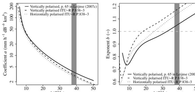
Figure 2.Values of coefficients in the relationship to convert specific attenuation to rainfall intensity for frequencies ranging from 6 to 50 GHz. The grey-shaded area denotes the 37.0–40.0 GHz range. Note the logarithmic vertical scale in the left figure. Here values have been computed from one data set of measured drop size distributions (p. 65 in Leijnse (2007c); solid lines). The values recommended by the International Telecommunication Union (ITU, 2005), meant for computing specific attenuation for given rain rates and for worldwide application, are also plotted (dashed and dotted lines).
on GitHub, are valid for vertically polarised signals (Fig. 2), which will usually be employed for microwave links. Utilis-ing these coefficients for horizontally polarised signals will generally only produce small errors in the retrieved rain-fall estimates. The values recommended by the International Telecommunication Union (ITU, 2005), meant for comput-ing specific attenuation for given rain rates and for world-wide application, are also plotted. Differences up to 10 % are found for the value of the exponentbfrom ITU (dashed and dotted lines) compared to that obtained from drop-size dis-tribution data from the Netherlands (solid lines).
For the link frequencies employed in this study (between 12.8 and 40.0 GHz) the value of the exponentbis close to 1 (Fig. 2, right). (Berne and Uijlenhoet, 2007), (Leijnse et al., 2008, 2010), and (Overeem et al., 2011) show that this near-linearity only leads to small errors in rainfall estimates.
The assumed temporal sampling strategy only provides a minimum and maximum received power over a given time interval. The goal is to obtain a reliable mean path-averaged rainfall intensity over this time interval. This is achieved by computing the mean path-averaged rainfall intensity as a weighted average:
hRi =αhRmaxi +(1−α)hRmini, (8) whereαis a coefficient that determines the relative contri-butions of the minimum (hRmini) and maximum (hRmaxi) path-averaged rainfall intensity (mm h−1) during a time in-terval. The values for Aa (2.3 dB) andα (0.33) have been taken from Overeem et al. (2013), who use a 12-day calibra-tion data set from June and July 2011 (which has not been used for validation). They compare daily link-based rainfall depths with gauge-adjusted radar retrievals to calibrate the rainfall retrieval algorithm.
3.6 Rainfall maps
Path-averaged rainfall intensities from microwave links are spatially interpolated to obtain rainfall maps. The user can choose to apply ordinary kriging (OK) employing a spherical variogram model (Overeem et al., 2013; Rios Gaona et al., 2015) or to apply inverse distance weighted (IDW) interpo-lation on link rainfall data. OK and IDW are well suited for dealing with heterogeneously distributed data locations. OK requires a variogram model, but unfortunately it is impossi-ble to robustly estimate such variograms for each time inter-val separately due to the sparsity of rainfall. Hence, a more robust procedure is followed. The parameter values can be supplied by the user or they can be computed as follows. The sill and range of an isotropic spherical variogram model have been expressed as a function of day of year (DOY) and du-ration (1–24 h) using a 30-year rain gauge data set from the Netherlands (Van de Beek et al., 2012). This data set does not overlap with the link data set. If needed the relationships can be extrapolated to time intervals shorter than 1 h. The nugget is set equal to 0.1 times the sill. Note that these equations and the optimal values of their coefficients have been found to be useful for the Dutch climate. Hence, they may need ad-justment for other climatic settings. See Appendix D for a detailed description of the interpolation algorithm.
0 50
N
Links, nearby link approachOutlier filter
km 1,416 link paths
20110910, 2030 − 2045 UTC 0.1
1.6 3.1 4.6 6.1 7.6 9.1
15−min rainfall depth
mm
0 50
N
Links, nearby link approach Outlier filter; Middle of link path km 1,416 points
20110910, 2030 − 2045 UTC
0.1 1.6 3.1 4.6 6.1 7.6 9.1
15−min rainfall depth
mm
0 50
N
Links, nearby link approach Outlier filter; Kriged map km 38,063 pixels of 0.9 km2
20110910, 2030 − 2045 UTC 0.1
1.6 3.1 4.6 6.1 7.6 9.1
15−min rainfall depth
mm
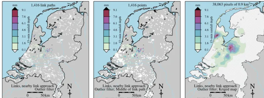
Figure 3.The figure illustrates how path-averaged link rainfall depths are interpolated to link rainfall maps. First, path observations (left panel) are assigned to points (centre panel). Next, ordinary kriging is applied to obtain rainfall maps (right panel). For time interval 20:30– 20:45 UTC on 10 September 2011.
can be visualised by using the functions provided in the pack-age. This is described in more detail in Appendix E.
4 Results
4.1 Illustration of steps in rainfall retrieval algorithm Here the steps in the rainfall retrieval are illustrated. Start-ing points are the minimum and maximum received powers over a given time interval (15 min in this case), as shown in Fig. 4a for one link during 24 h. As expected, there is a strong negative correlation between the minimum received powers and the path-averaged gauge-adjusted radar rainfall intensi-ties, considered to be the ground truth. Next, the corrected received powers and the reference level are shown (Fig. 4b). In this particular example the received powers are hardly cor-rected. A decrease around 08:30 UTC, probably not related to rainfall, is corrected for. In contrast, a rain-induced de-crease just before 17:00 UTC is removed. The mean path-averaged link rainfall intensities (Fig. 4d) and the cumulative link rainfall depths (Fig. 4e) correspond well with the gauge-adjusted radar-based values. In total approximately 60 mm was observed, resulting from two convective events with tens of millimetres in a couple of hours.
4.2 Rainfall mapping
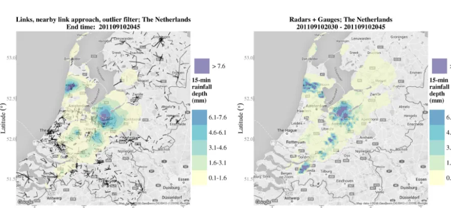
Link rainfall maps are compared to gauge-adjusted radar rainfall maps in Figs. 5 and 6 for 15 min and daily rainfall ac-cumulations respectively. These are obtained using ordinary kriging with a climatological spherical variogram model. The left panels show the link-based rainfall maps with the loca-tions of the employed links for the nearby link approach with outlier filter. The radar rainfall maps are given in the right panel. The cellular communication network is able to detect the rainfall patterns for the 15 min interval, although
devi-ations are found with respect to radars combined with rain gauges. Note that some large areas do not have link data. The daily rainfall maps are from 10 September 2011, 08:00 UTC, to 11 September 2011, 08:00 UTC, and reveal link-based rainfall depths larger than 26.0 mm. These local high rain-fall depths occurred in a few hours, i.e. convective rainrain-fall. In general, the link network is able to correctly determine the spatial rainfall patterns. These examples demonstrate a successful application of microwave links to estimate rain-fall. Figure 7 illustrates the capability of the rainfall mapping functions to produce a (local) rainfall map of high graphical quality.
4.3 Sensitivity analyses
For all sensitivity analyses the same values forAa (2.3 dB) andα(0.33) are employed, i.e. as obtained for the nearby link approach with outlier filter using the default parameter values (Table 3). Validations are performed on 15 min path-averaged link rainfall depths or link rainfall maps from the 12-day validation data set (Overeem et al., 2013). No thresh-old values regarding the minimum rainfall depths are applied in the comparisons. Metrics are computed for residuals, i.e. the link minus the gauge-adjusted radar rainfall depths. The sensitivity analyses are based on 12 rainy days from the sum-mer. Such analyses may yield different results for other sea-sons and rainfall types.
4.3.1 Nearby link approach wet–dry classification A sensitivity analysis is performed for the two threshold values of the wet–dry classification, where median(1P )
Figure 4.From received signal powers to cumulative rainfall depths (one day, one link): minimum and maximum received powers and
path-averaged, gauge-adjusted radar rainfall intensities(a); corrected minimum and maximum received powers, reference signal levels, and
path-averaged, gauge-adjusted radar rainfall intensities(b); minimum and maximum path-averaged link rainfall intensities(c); mean
path-averaged link and gauge-adjusted rainfall intensities(d); cumulative path-averaged link and gauge-adjusted radar rainfall depths(e); map
with location of microwave link in the city centre of Amsterdam, the Netherlands(f). Period is 30 August, 08:00 UTC–31 August, 08:00 UTC
(2012).
Figure 5.Fifteen-minute rainfall maps from 10 September 2011, 20:30–20:45 UTC, for links only (left) and radars plus gauges (right) for
the Netherlands. Spatial resolution is approximately 0.9 km2. Values below 0.1 mm are not shown. The lines denote the locations of the
Figure 6.Daily rainfall maps for links only (left) and radars plus gauges (right) for the Netherlands. Spatial resolution is approximately
0.9 km2. Period is 10 September, 08:00 UTC–11 September, 08:00 UTC (2011). Values below 1.0 mm are not shown. The lines denote the
locations of the employed microwave links (left). This figure is part of the working example.
Figure 7.Illustration of plotting capability of R visualisation func-tion “RainMapsLinksTimeStep” in package RAINLINK: 15 min rainfall map from 10 September 2011, for links only for
Amster-dam, the Netherlands. Spatial resolution is approximately 0.9 km2.
Values below 0.2 mm are not shown. The lines denote the locations of the employed microwave links. The number at the red cross is the rainfall depth at that location, of which the name is provided in the title caption. This figure is part of the working example.
potentially become positive, this will hardly happen or only small positive values will be obtained. If both threshold val-ues are 0 dB (km−1) this can therefore be considered repre-sentative for the situation without wet–dry classification.
The 2-D contour plots in Fig. 8 display relative mean error (%; black lines) and coefficient of variation (CV) or squared correlation coefficient (ρ2) (colours) in path-averaged 15 min rainfall depths as a function of median(1P )
and median(1PL). The default threshold values are indicated by the black dot. Given the resolution of 1 dB, the default value for median(1P ),−1.4 dB, implies that median(1P )
should be lower than−1 dB (hence the black dot is plotted at 1 dB). In order to focus on the performance of the wet–dry classification with respect to the situation without wet–dry classification, the outlier filter has not been applied here. A wet–dry classification generally leads to a clear improvement in terms ofρ2and CV upon a situation without wet–dry clas-sification.
The contour plots show that application of median(1PL) is not necessary and that the best results are obtained for median(1P )values around−4 dB, i.e. much lower than the default value. Note that the default values ofAaandαhave been used, where an outlier filter was applied. This may be the reason for the variability in relative mean errors. Find-ing optimal values ofAa and α for every combination of median(1P )and median(1PL)was considered too compu-tationally demanding and could have compensated for errors in wet–dry classification for each combination of both thresh-old values.
There-5.0 5.5 6.0 6.5 C V −5 −4 −3 −2 −1 0
−2 −1.5 −1 −0.5 0
Sensitivity analysis 12 days
Median(∆PL) (dB km )−1
M ed ia n ( ∆ P ) ( d B ) ● 0.32 0.34 0.36 0.38 0.40 ρ2 −5 −4 −3 −2 −1 0
−2 −1.5 −1 −0.5 0
Sensitivity analysis 12 days
Median(∆PL) (dB km )−1
Me d ia n ( ∆ P ) ( d B ) ●
Figure 8.Sensitivity analyses of the threshold values for the wet–dry classification. The 2-D contour plots display relative mean error (%;
black lines) and, in colours, CV (left) orρ2(right) in path-averaged 15 min rainfall depths as a function of median(1P )and median(1PL).
The default threshold values are indicated by the black dot. No outlier filter has been applied.
−300 −200 −100 0
0.35 0.40 0.45 0.50 0.55 0.60
Ft (dB km−1 h)
ρ
2
−300 −200 −100 0
3.0 3.5 4.0 4.5 5.0 5.5
Ft (dB km−1 h)
C
V
−300 −200 −100 0
−10
0
10
20
Ft (dB km−1 h)
Relativ
e mean error (%)
−300 −200 −100 0
0.0 0.2 0.4 0.6 0.8 1.0
Ft (dB km−1 h)
Fraction of data left
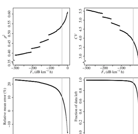
Figure 9. Sensitivity analyses of the threshold value for the
out-lier filter. Performance in terms ofρ2, CV, and relative mean error
(%) as a function of outlier filter threshold for path-averaged 15 min rainfall depths. The grey vertical line indicates the default threshold value chosen for the results in this paper. Also shown is the frac-tion of data which is left after applying the outlier filter for a chosen threshold value.
fore, this step can now also be discarded by supplying a func-tion argument. In this step the previous two time intervals and the next time interval are classified as wet if the present time interval is rainy and has more than 2 dB of attenuation for the link under consideration.
4.3.2 Outlier filter
Performance of link rainfall estimates clearly deteriorates if the outlier filter is not applied. The CV of the residuals is much larger, 6.03, theρ2is much lower, 0.35, and the relative bias in the mean becomes much larger, 24.2 % (compare to previous paragraph). The latter may be related to the fact that
Aaandαhave been calibrated on a data set where the outlier filter has been applied.
Now the performance for a wide range of threshold val-ues of the outlier filter is investigated for path-averaged 15 min rainfall depths. For the default threshold value of −32.5 dB km−1h−1, denoted by the grey line, good results are obtained in terms of ρ2 and CV (Fig. 9). Results im-prove for increasing threshold values at the expense of a se-vere decline in the amount of link data. The best choice for a threshold value is somewhat arbitrary, i.e. a range of val-ues gives good results, while still having many link data. The relative mean error decreases from more than +20 % to less than−15 % fromFt= −300 to 0 dB km−1h−1. If for each value ofFtthe coefficientsAaandαwould have been cali-brated, the relative mean error would be expected to be more constant. Apparent are the jumps inρ2and CV for certain values ofFt. It seems that these are related to some very large “rainfall depths”, which point to malfunctioning links. Note thatF is the cumulative difference between a link’s specific attenuation and that of the surrounding links. Hence, such jumps for strongly negative values ofFtare likely not caused by rain or (sources of) errors affecting a whole region. 4.4 Performance of ordinary kriging versus inverse
distance weighted interpolation
rain-fall maps (0.9 km2), which are aggregated to daily rainfall maps (0.9 km2). The nearby link approach with outlier filter and default parameter values has been applied. These maps are computed for two interpolation methodologies: (1) OK with a spherical climatological variogram model, i.e. the de-fault method; (2) IDW interpolation with an inverse distance weighting power of 2.0.
First, the 15 min rainfall maps are studied. The follow-ing metric values are obtained for IDW: relative mean error of 8.3 %, CV of 3.30, and a ρ2 of 0.41. OK performs bet-ter, since the relative mean error is clearly lower (1.5 %), CV is similar (3.29), and ρ2 is clearly higher (0.48). De-spite the high spatial resolution of the obtained rainfall maps (0.9 km2) compared to the link density, still reasonable re-sults are obtained in terms ofρ2, but values of CV are high.
Next, the daily rainfall maps are investigated. The follow-ing metric values are obtained for IDW: relative mean error of 8.2 %, CV of 0.51, and aρ2of 0.70. OK performs some-what better, since the relative mean error is clearly lower (1.4 %), CV is slightly larger (0.54), and ρ2 is somewhat higher (0.73). Hence, the improvement of OK with respect to IDW is particularly evident at the 15 min scale. Note that the results for the daily timescale are much better than those for the 15 min timescale. The performance of IDW could be-come better if another value of the inverse distance weighting power would be selected.
5 Discussion
5.1 Computation time
Using one processor (Intel i7; Linux operating system) the entire processing up to and including the interpolation takes around 10 min, i.e. to obtain 15 min link-based rainfall maps for 40 h based on data from on average 2381 links and 2473 links in total (representing 1527 unique link paths). Not ap-plying a wet–dry classification leads to a decrease in compu-tation time of 1 min. Most time is consumed by the OK in-terpolation (8 min). The IDW inin-terpolation only takes 2 min (for an inverse distance weighting power of 2.0). A similar amount of time would be needed in case multiple processors would be used to run multiple periods, each processor run-ning its own period. In order to reduce computational time it could also be worthwhile to divide a region into subregions, particularly to speed up the wet–dry classification. Another option would be to transfer the algorithm to a high-level pro-gramming language.
5.2 Transferability of code
The developed rainfall retrieval algorithm or its parameter values will likely need adaptation for (optimal) rainfall es-timation for other networks and climates around the world. Nevertheless, many networks have similar characteristics as those in the Netherlands. A 15 min sampling strategy, either
instantaneous or minimum and maximum values, is common and has been used in several other networks (e.g. Messer et al., 2006; Leijnse et al., 2007a; Messer and Sendik, 2015). We advocate a pragmatic approach to first apply this algo-rithm to data from those networks with minimum and maxi-mum received signal levels and assess the quality of the de-rived rainfall maps. This is certainly relevant for areas (e.g. developing countries) where few reference rainfall data are available to calibrate the rainfall retrieval algorithm. Sub-optimal parameter values or interpolation methods may still provide meaningful rainfall estimates for other networks or climates.
As a next step the parameters of the algorithm could be adapted to local conditions, for instance based on recommen-dations from the International Telecommunication Union (ITU, 2005). Then it could be decided whether further modi-fications of the algorithm would be needed or not. For poorly gauged regions we suggest optimising the algorithm, includ-ing interpolation methodology, employinclud-ing data from a re-gion with a similar climate and network, for which sufficient ground-truth rainfall data are available.
Coefficients and thresholds have been optimised for 15 min intervals; hence their values may not be appropriate for other time intervals. Their values can be easily changed by modifying function arguments.
Even if network characteristics are very different, e.g. in terms of sampling strategy, large parts of our code could still be used to develop algorithms suited for the specific needs of these networks. Although the rainfall retrieval algorithm contains several empirical parameters, the developed meth-ods are not merely statistical in nature. Their general ples hold for other networks as well. For instance, the princi-ple of the wet–dry classification, where data from surround-ing links are used to distsurround-inguish between wet and dry peri-ods, makes use of the general fact that rainfall is correlated in space, although decorrelation distances can vary between different climates.
which also holds for the maximum received and transmitted powers.
Ideally, the employed values foraandbshould match the polarisation of the link. If information on the latter is avail-able, the code could be easily adapted to incorporate this. 5.3 Parameter values
Table 3 gives an overview of the parameters of the rainfall retrieval algorithm, their default values, and the factors in-fluencing them. This can help to assess which parameters will change for other regions and networks. Some parame-ters are already modelled as function of frequency, others do not seem to be sensitive to frequency, whereas again others should ideally be optimised for different frequencies. 5.3.1 Wet–dry classification with nearby link approach Some of the signal fluctuations that occur in dry weather may also occur during rainy periods. The algorithm does not cor-rect for such errors. Furthermore, nearby links may suffer si-multaneously from signal fluctuations not caused by rainfall, resulting in a poor performance of the nearby link approach. The parameters concerning the wet–dry classification have been optimised using data from another period and are based on received signal level data stored at 0.1 dB resolution (Overeem et al., 2011). These values have been applied in Overeem et al. (2013) and in the current manuscript to an in-dependent data set from another brand of links with slightly different antenna covers and a coarser 1 dB power resolution. The sensitivity analysis shows that the parameter values from Overeem et al. (2011) are suboptimal but give a clear im-provement in link-based rainfall estimates compared to the case without wet–dry classification.
The chosen radius depends on the spatial correlation of rainfall and is, hence, not frequency dependent. Because net-works are designed in such a way that 1P will be simi-lar for different microwave frequencies, lower frequencies are utilised for longer link paths and vice versa. Lower fre-quencies experience less rainfall-induced specific attenua-tion compared to higher frequencies. Hence, median(1P )
is nearly independent of frequency.
Ideally, a sensitivity study should be carried out to find op-timal threshold values for the wet–dry classification in case of other networks and climates. This will be computationally expensive in case of large data sets.
It is to be expected that the nearby link approach will also work for other temporal resolutions than 15 min. This may require a smaller radius and a higher link density for higher temporal resolutions and may allow a larger radius and lower link density for lower temporal resolutions. For data sampled at very high frequencies, i.e. 1 s, the nearby link approach may become too computationally expensive. This could be circumvented by first averaging signal attenuations over longer durations before applying this approach.
5.3.2 Reference level determination
Note that a default 24 h period is considered for determining the reference level and for one step in the nearby link ap-proach. Such a relatively long period is chosen, among other reasons, to increase the probability to obtain at least 2.5 h of dry periods, which helps to determine the reference level more accurately. Note that both periods can be modified. 5.3.3 Outlier filter
The filter to remove outliers deals with specific attenuation; i.e. it does not explicitly take into account frequency. It is also suitable for other time interval lengths. Nevertheless, its threshold value is very high, which makes it unlikely that actual rainfall is filtered out accidentally, irrespective of the employed frequency. The outliers are likely caused by mal-functioning links. Perhaps melting precipitation also plays a role. Hence, it makes sense to apply a frequency-independent threshold value. Note that the threshold value may need to be optimised for other networks and climates. The sensitivity analysis on a 12-day data set shows that the chosen default value ofFt is suitable but a range of values shows a similar performance.
5.3.4 Wet antenna attenuation and sampling strategy The wet antenna attenuation correctionAawill not only com-pensate for wet antennas. The value ofAafound in the cali-bration will also be influenced by other errors. Moreover, in case of rain along the link path no, one, or both antennas can be wet, whereas this correction is always applied, andAa it-self has also been optimised on data where the number of wet antennas can vary. In addition, the correction does not depend on rainfall intensity. Hence, applyingAashould be seen as a pragmatic approach towards correcting for wet antennas.
The coefficient α is employed to obtain mean path-averaged rainfall intensities from minimum and maximum path-averaged rainfall intensities and is expected to depend on the time variability of rainfall. Note that the value ofα
presented here is based on data available at 15 min time in-tervals. It is expected that this value will be different for disparate time intervals. Messer et al. (2006) use the known distribution of rainfall intensities at the point scale to weigh minimum and maximum received signal levels.
(gauge-adjusted) weather radar data, which may provide full cov-erage over the network, as in Overeem et al. (2013). Alter-natively, path-averaged rainfall intensities may be estimated from rain gauge data. This may require a dedicated research experiment (Minda and Nakamura, 2005; Wang et al., 2012), preferably with several rain gauges along the link path.
Overeem et al. (2011) utilise a research link with high tem-poral resolution for testing the proposed rainfall retrieval al-gorithm. By applying the rainfall retrieval algorithm, mean path-averaged rainfall intensities can be derived. These can be compared to the corresponding true values obtained from the received signal powers sampled at 10 Hz. Hence, the same instrument, a microwave link, is used to assess the abil-ity of the retrieval algorithm to deal with the sampling strat-egy. Since the same instrument is used representativeness er-rors are not present. The probability distribution of minimum and maximum rainfall intensities could be studied in order to obtain more reliable mean rainfall intensities. Moreover, such an experiment may also help to assess attenuation due to wet antennas caused by dew or rain, its dependence on rainfall intensity or antenna cover type, and the time it takes for antennas to dry following a rain event. Preferably a rain gauge or disdrometer should be available near the antenna. A research link is particularly useful when the microwave fre-quency, path length, and antenna cover are representative of the links in a cellular communication network. Finally, see, for instance, Leijnse et al. (2007b, 2008) and Schleiss et al. (2013) for other wet antenna attenuation correction methods. 5.3.5 Interpolation methodology
The employed interpolation methodology, ordinary kriging, may not be specifically suited for other regions with different rainfall climatologies. The methodology developed in Van de Beek et al. (2012) could be optimised for other climates. This requires long rainfall time series. The assumed stationarity and isotropy will often be violated (Schuurmans et al., 2007). However, violation of assumptions does not automatically imply that the interpolation method is not useful. Further, the path-averaged link rainfall intensities are assumed to be point measurements. Hence, it is recommended to improve the in-terpolation methodology, e.g. by treating the rainfall values as line observations instead of as point observations, which is expected to have the largest impact at local scales for areas with high link densities or at areas with long links. Using data from the same 12 days as employed in Overeem et al. (2013), Rios Gaona et al. (2015) find that link rainfall retrieval errors themselves are the source of error that contributes most to the overall uncertainty in rainfall maps from a commercial link network. Errors due to mapping, i.e. interpolation method-ology and link density, play a minor, albeit non-negligible role for the same network as utilised in this study. Hence, de-spite the limitations of the interpolation methodology its use-fulness has been confirmed (Overeem et al., 2013). Further, Rios Gaona et al. (2015) study the performance of simulated
link rainfall maps as a function of link density. They show that even for low spatial link densities reasonable results can still be obtained.
It may be interesting to apply a tomographic approach in order to obtain link-based rainfall maps (Zinevich et al., 2008; Cuccoli et al., 2013). Such an approach can potentially reconstruct the two-dimensional distribution of rainfall from a set of one-dimensional transmission data from many dif-ferent (nearby or even intersecting) paths (Giuli et al., 1991). Hence, it would take the line character of the attenuation measurements into account, in contrast to the current ap-proach where a line measurement is assigned to a point at the middle of the link path.
The estimated sill and range will become less accurate by extrapolating to time intervals shorter than 1 h, such as 15 min. Villarini et al. (2008) use rain gauge data from Eng-land to quantify spatial correlation for short time intervals, e.g. 1 and 15 min. These kind of studies can be useful to im-prove the interpolation of link-based rainfall intensities. 5.3.6 R–krelationship
The relationship between path-averaged rainfall intensity and path-averaged specific attenuation is commonly employed in other studies. The provided parameter values ofa andbare available for frequencies ranging from 1 to 100 GHz. The value of the exponentbis close to 1 for the frequencies em-ployed in this study, which range from 12.8 to 40.0 GHz. Frequencies between 37.0 and 40.0 GHz are denoted by the grey-shaded area in Fig. 2, which contains 81 % of the links from the working example, having values ofbvery close to 1 (right). For other frequencies the corresponding value of
b often deviates more from 1 (Fig. 2, right). High rainfall variability along the link path will lead to overestimation for
b <1 and underestimation for b >1 (Leijnse et al., 2008; Uijlenhoet et al., 2011).
6 Conclusions
It has been shown in several studies that microwave links from cellular communication networks can be used to retrieve rainfall information. For instance, country-wide (≈35 500 km2) 15 min rainfall maps can be obtained from received signal powers of microwave links (Overeem et al., 2013). In this paper a detailed description is given of the al-gorithm of Overeem et al. (2013). The accompanying code is made publicly available as the R package RAINLINK via GitHub under the condition of version 3 or later of the GNU General Public License. The modular programming facili-tates users to adapt the code to their specific network and climate conditions or to only employ one or some functions of RAINLINK. We hope that RAINLINK will promote the application of rainfall monitoring using microwave links in poorly gauged regions around the world.
We invite researchers to contribute to RAINLINK to make the code more generally applicable to data from different net-works and climates. Ideally, the code should be tested on data sets containing all seasons, for varying networks and regions. Such an endeavour worldwide is currently difficult to achieve. It would require an enormous effort and it would also require data sharing among researchers, which is still not that easy to accomplish due to confidentiality requirements often imposed by telecommunication companies.
One may wonder whether the technology is bound to dis-appear due to the introduction of fibre optical cable networks. For instance, for the provided link data set the majority of the links does not exist anymore due to network renewal and deployment of underground fibre optical cable networks. Whereas the Netherlands is at the forefront internationally concerning deployment of underground fibre optical cable networks for telecommunication between base stations, the country is expected to still have several thousands of links (from cellular telecommunication companies and others) in 2025. For other countries and continents the uptake of fibre optics will be significantly slower, lagging behind at least 5– 20 years. Moreover, construction of fibre optical cable net-works may not be feasible or economically viable in many mountainous or rural areas around the world. Therefore, we expect this type of cellular communication infrastructure to still be around for several decades worldwide (Ralph Kop-pelaar, T-Mobile NL, personal communication, 2016). Why not attempt to use this existing infrastructure as a comple-mentary source of rainfall information, in particular in those areas around the world with very few rain gauges, let alone weather radars?
Although rain gauges, radars, and satellites have been specifically designed to measure rainfall, all of these instru-ments face their own challenges. It is well known that radar rainfall estimates generally deteriorate for longer ranges from the radar. Geostationary satellite observations have a time resolution of typically 15 min but are often very indi-rect (e.g. estimates through cloud physical properties;
Roe-beling and Holleman, 2009). Low-Earth Orbit satellites usu-ally have long revisit times. Despite (new) satellite missions, microwave link data can still become important for ground validation of or merging with satellite rainfall products. For instance, the IMERG product of the new GPM mission pro-vides gridded rainfall products every 30 min covering 60◦N– 60◦S with a spatial resolution of 0.1◦ (Hou et al., 2014; Rios Gaona et al., 2016). This is certainly a major step for-ward with respect to TRMM, but one has to recognise that the rainfall retrieval algorithm heavily relies on temporal in-terpolation and, depending on the product, additional data sources, such as rain gauges, since the actual satellite revisit time is typically several hours. Moreover, links measure rain-fall close to the ground, which is not the case for weather radar and satellites, and at spatio-temporal scales relevant for meteorology and hydrology (typically 1 s–15 min; 0.1– 20 km). Even if rain gauges are present, the number of links will often be an order of magnitude larger than the num-ber of rain gauges in a region. The larger spatial density of links has been demonstrated in our previous work to com-pensate for their lower accuracy with respect to rain gauges. Hence, rainfall information from cellular telecommunica-tion networks is promising for hazardous weather warning, flood forecasting, food production, drought monitoring, etc. Finally, although it is indeed difficult to obtain transmitted and received signal level data from telecommunication com-panies, researchers have managed to obtain data for a lim-ited, but expanding, number of countries (namely, Australia, Brazil, Burkina Faso, Czech Republic, France, Germany, Is-rael, Kenya, Pakistan, Sweden, Switzerland, and the Nether-lands).
To conclude, we feel that merging of rainfall data from different sources (if available) will often yield the best rain-fall estimates. For instance, satellite data could be used for wet–dry classification to prevent non-zero link-based rain-fall estimates during dry periods (Van het Schip et al., 2016). We believe that the main potential for rainfall estimation us-ing microwave links is found in areas with few surface rain-fall observations. In addition, development of a merged link-satellite rainfall product seems an interesting opportunity.
Data availability
The data from the “Radar precipitation climatology” (Overeem et al., 2016b), i.e. the gauge-adjusted radar rainfall data set, as well as the “RAINLINK microwave link data set” (Overeem et al., 2016a), are freely available for all parties. The radar data set can be obtained from http://climate4impact.eu/impactportal/data/catalogbrowser. jsp?catalog=http://opendap.knmi.nl/knmi/thredds/
Appendix A: Required data format
The code is designed for estimating rainfall from minimum and maximum received powers over time intervals of a given length, as that is the way in which cellular telecommunica-tion companies typically store their data. The time interval does not have to be an integer but should be equidistant. The time interval length is automatically computed by the RAIN-LINK package. For each link and time interval the following variables are needed: microwave frequency f (GHz), mini-mum and maximini-mum received powerPminandPmax(dBm), date and end time of observation (YYYYMMDDhhmm, i.e. year (2011), month (09), day (11), hour (08), minutes (00): 201109110800), path length L (km), coordinates (latitude and longitude) of start and end of link in WGS84 (degrees; default, also another coordinate system may be chosen), and unique link identifier (ID), which should remain the same over the entire processed period. A full-duplex link should have two IDs, one for each link direction. Note that a header should be provided as given in the data file from the example. The order of the columns does not matter, as long as the vari-able name matches the column. IDs are handled as strings. Hence, not only integers, but, for instance, also alphanumeric IDs can be used.
A user can supply microwave link data for an arbitrary pe-riod. Note that missing link data are allowed; i.e. the code will work when a time interval has no data. However, many missing data or a too short period may lead to rainfall inten-sities not being calculated.
In this paper data from one network have been utilised. In case data from more networks, either from the same or from different providers, are available, these can simply be combined into one data frame. The only requirements are that unique link identifiers are employed and that these networks use the same sampling strategy.
Appendix B: Preprocessing of link data
The processing starts with the preprocessing of link data us-ing the function “Preprocessus-ingMinMaxRSL”, which does the following.
1. Microwave link data are supplied as function argument. 2. Select only those links with microwave frequencies in chosen range (here 12.5–40.5 GHz; almost all T-Mobile NL links used to operate in this range). The chosen fre-quencies can be supplied as function arguments. 3. For each unique link identifier a time interval is
re-moved if it contains more than one record.
4. If no link data are available anymore for the selected unique link identifier, perform the previous step for the next unique link identifier.
5. For each unique link identifier it is checked whether its frequency, link coordinates, or path length vary during the considered period. If this is the case for one of these variables, the link is discarded for this particular consid-ered period.
6. A data frame is provided as output.
7. Repeat these steps for each unique link identifier.
Appendix C: Wet–dry classification with nearby link approach
A step-by-step description of the classification algorithm (function “WetDryNearbyLinkApMinMaxRSL”) is given below and mainly obtained from Overeem et al. (2011). The classification is run for each link for the period for which data are provided. Note that running this wet–dry classification is optional.
1. The link coordinates are converted to an azimuthal equidistant cartesian coordinate system (easting and northing of start of link, easting and northing of end of link; km).
2. Select a link.
3. All links for which both end points are within a chosen radius (default 15 km) from either end of the already selected link are selected as well.
4. Continue if at least three surrounding links have been selected for the considered time interval for which the link in step 2 has data, otherwise the link is not used for that time interval. If the link is part of a full-duplex link, the other link is counted as surrounding link.
5. Calculate the attenuation1P =Pmin−max(Pmin)and specific attenuation1PL=Pmin−max(PL min) for each link and each time interval. max(Pmin) is the maximum value ofPminover the previous number of hours includ-ing the present time interval (default 24 h). Note that max(Pmin)is only computed if at least a minimum num-ber of hours of data are available (default 6 h); otherwise it is not computed and no rainfall intensities will be re-trieved.
6. The median values of1P and1PLare computed over all selected links for each time interval.
7. If median(1PL) <−0.7 dB km−1and median(1P ) < −1.4 dB the time interval is classified as wet for the link selected in step 1.
9. All time intervals that have not been classified as wet are classified as dry for the link selected in step 1. 10. Repeat these steps for all other links.
Note that a radius of 10 km is used in Overeem et al. (2011), whereas a default radius of 15 km is used here and in Overeem et al. (2013), which allows estimating rainfall in ar-eas with lower spatial link densities. The 15 km radius is rep-resentative of the decorrelation distance of convective rain-fall in the Netherlands in case of a time interval of 15 min. For the often occurring stratiform rainfall this distance will be (much) longer. Step 4 has been slightly altered with re-spect to Overeem et al. (2011).
The threshold values in steps 7 and 8 have been obtained from Overeem et al. (2011), who optimise them by visual comparison with the gauge-adjusted radar data set of path-averaged rainfall intensities employing data from 2009 (NEC links with 0.1 dB power resolution). Step 8 was used because rainfall is generally correlated in time, and sometimes very local, so that it does not occur at surrounding links.
If the algorithm would be rerun for another period, for in-stance one time interval later, this can result in different rain-fall estimates compared to the preceding run. This is due to step 8 of the wet–dry classification methodology, which may also classify the previous 30 min as rainy. In order to obtain the same rainfall estimates for different runs, the algorithm would need to be slightly modified or one should wait 30 min before applying the algorithm. Another option is to not ap-ply step 8, which can be supplied as function argument. The rainfall retrieval algorithm is suitable for real-time applica-tion, for which the reclassification of previous time intervals is of no consequence, because rainfall intensity of present time interval is of interest.
Appendix D: Interpolation methodology
Here an extensive description of the interpolation algorithm is given, which is carried out by calling the function “Inter-polation”. It performs the following steps.
1. Convert the supplied interpolation grid with coordinates (longitude and latitude; two columns) to an azimuthal equidistant cartesian coordinate system. In the example the interpolation grid is in WGS84 (degrees). A radar grid is used, where the coordinate of each grid cell rep-resents the middle of the radar pixel. The coordinates of the supplied link data are also converted to an az-imuthal equidistant cartesian coordinate system (easting and northing; km).
2. Select the mean path-averaged link rainfall intensities for each time interval.
Then it calls the subfunction “IntpPathToPoint”, which does the following:
1. Compute the coordinates belonging to the middle of the links.
2. Determine the unique coordinates of the middle of the links.
3. Calculate the average rainfall intensity for each unique set of coordinates. This implies that data from full-duplex links are averaged. If another link happens to have the same middle of the link path, its rainfall in-tensity is taken into account in the averaging.
Next, three different interpolation methodologies are avail-able, which can be chosen by supplying a function argument: 1. Inverse distance weighted interpolation on link rainfall data (subfunction “IDW”). The inverse distance weight-ing power should be supplied as function argument. 2. Ordinary kriging with spherical variogram model. Its
parameter value nugget, sill, and range can be defined by the user as function arguments.
3. Ordinary kriging with spherical variogram model with climatological parameter values based on a 30-year rain gauge data set. These are computed for the DOY as ob-tained from the input data frame with microwave link data, thus taking into account seasonality in spatial rain-fall correlation. The subfunction “ClimVarParam” com-putes these parameter values.
For the last methodology the spherical variogram parame-ters can be computed as follows (power-law scaling in cosine function parameter; Van de Beek et al., 2012):
r= 15.51D0.09+2.06D−0.12cos 2π(DOY−7.37D
0.22)
365
!!4
, (D1)
C=
0.84D−0.25+0.20D−0.37cos
2π(DOY−162D−0.03) 365
4
, (D2)
C0=0.1C, (D3)
wherer is the range (m), C is the partial sill (mm2h−2), C0is the nugget (mm2h−2), DOY is day of year, andDis the duration (h), i.e. the time interval of the rainfall inten-sities which are to be interpolated. The nugget is basically the semi-variance at zero distance, which can be interpreted as very-fine scale variability or as measurement uncertainty. The sill is the variance at very large distances, and the range is the distance at which the variance does not increase any more (this is equivalent to the distance beyond which the field is completely decorrelated, i.e.ρ(r)=0).
The spherical variogram takes the following form:
γ (h)=
C "
3 2
h
r −
1 2
h
r 3#
+C0 if h≤r
C+C0 if h > r,
(D4)
The interpolation is performed for the provided grid. For ordinary kriging the 50 (default value) nearest observations are used in order to reduce computational time (subfunction “OrdinaryKriging”). Negative rainfall values occur regularly, and are replaced by zero values. Finally, the function “Inter-polation” only gives the rainfall intensity (mm h−1) as out-put. Each row corresponds to the same row from the interpo-lation grid.
Appendix E: Visualisation of rainfall maps
The rainfall maps can be visualised using the functions de-scribed for step 8 in Table 1. Both link and radar rainfall