www.the-cryosphere.net/10/29/2016/ doi:10.5194/tc-10-29-2016
© Author(s) 2016. CC Attribution 3.0 License.
Virtual radar ice buoys – a method for measuring fine-scale
sea ice drift
J. Karvonen
Finnish Meteorological Institute (FMI), Helsinki, PB 503, 00101, Finland Correspondence to: J. Karvonen ([email protected])
Received: 27 May 2015 – Published in The Cryosphere Discuss.: 8 September 2015 Revised: 5 November 2015 – Accepted: 12 December 2015 – Published: 15 January 2016
Abstract. Here we present an algorithm for continuous ice drift estimation based on coastal and ship radar data. The ice drift is estimated for automatically selected ice targets in the images. These targets are here called virtual buoys (VBs) and are tracked based on an optical flow method. To maintain continuous ice drift tracking new VBs are added after a given number of VBs have been lost; i.e. they can not be tracked reliably any more. Here we also apply the algorithm to data of three test cases to demonstrate its capabilities and proper-ties. Two of these cases use coastal radar data and one ship radar data. Ice drift velocity and direction information de-rived from the VB motion are computed and compared to the prevailing ice and weather conditions. Also a quantity mea-suring the local divergence or convergence is computed for some VBs to demonstrate the capability to estimate derived kinematic sea ice parameters from VB location time series. The results produced by the algorithm can be used as an in-put for estimation of the dynamic properties of sea the ice field, such as ice divergence or convergence, shear, vorticity, and total deformation.
1 Introduction
Sea ice motion is an important parameter, because ice dy-namics has a major effect on the nature of sea ice. Ice motion can cause ice pressure, which in turn contributes to ice de-formation, or diverging ice motion can cause opening of ice (cracks, leads). The main goal of this study was to develop and test an algorithm suitable for continuous operational ice drift monitoring based on radar data and to demonstrate it for a few test data sets from coastal and ship radars.
If necessary, radar platform (ship) motion can be compen-sated based on the geoinformation (GPS (Global Positioning System) position of each radar frame). However, large ship motion is not desirable because the radar signal is rapidly at-tenuated as a function of the range or, in the worst case, the two radar images with a given time gap between them are not overlapping any more. If ship motion is not compensated then the ice drift with respect to the ship is measured, like in the ship radar test case in this study.
Many publications on ice drift from Synthetic Aperture Radar (SAR) imagery and other satellite-borne Earth Ob-servation (EO) data have been published. The motion esti-mation is based on detecting the same features in two ad-jacent images (e.g. Fily and Rothrock, 1987; Kwok et al, 1990; Sun, 1994; Thomas et al., 2004; Haarpaintner, 2006; Thomas et al., 2008; Karvonen, 2012). Motion vector estima-tion for weather radar data has also been studied, e.g. in Peura and Hohti (2004). Sea ice drift and object tracking from coastal radars have been studied earlier: e.g. in Okhotsk Sea in Tabata et al. (1980), by matching of prominent features preserved from image to another; in the Chukchi Sea near Barrow, Alaska, in MV et al. (2013), using Lucas–Kanade optical flow algorithm (Lucas and Kanade, 1981) for fea-tures detected by Harris corner/edge detection (Harris and Stephens, 1988) algorithm; and in the Baltic Sea in Karvo-nen (2013a), using a combination of phase correlation and normalized cross-correlation. Coastal radar data for sea ice analysis in the Canadian Arctic have been utilized in Shapiro (1976), Shapiro and Metzner (1989), Mahoney et al. (2007), Druckenmiller et al. (2009), and Mahoney et al. (2015).
es-timates are inter/extrapolated values. The motion detection methods are computationally intensive but in principle easy to parallelize due to the local nature of the computations.
In our earlier studies (Karvonen, 2013a; Karvonen et al., 2013) we have used data with longer temporal differences (10–30 min) than here and an algorithm based on cross-correlation techniques. This approach was directly adapted from techniques used for ice drift estimation from SAR im-agery (Thomas et al., 2004, 2008; Karvonen, 2012). How-ever, with a finer temporal resolution sub-pixel resolution would be desirable, and it can not be achieved using cross-correlation techniques without suitable interpolation of the results. This interpolation needs to be nonlinear, thus also requiring a larger support area than a simple linear interpola-tion. Optical flow algorithm in turn inherently gives the esti-mates with a sub-pixel resolution. For this reason we found the optical flow approach better suitable for sea ice drift anal-ysis from radar imagery of fine temporal resolution. Com-pared to our earlier algorithms (Karvonen, 2013a; Karvonen et al., 2013) we also get a better (sub-pixel) spatial and tem-poral resolution of the ice drift estimates.
This optical flow algorithm also enables continuous opera-tional ice drift monitoring. The algorithm automatically adds virtual buoys (VBs) as their number decreases under a given number and the monitoring can be continued for the ice sea-son without any human intervention. Based on the automati-cally performed ice drift analysis near-real-time information, e.g. on local convergence or divergence (closing or opening ship track), can be delivered for navigation in the area. Also the radar image data can automatically be stored and trans-mitted with a shorter time interval when the ice is moving or deforming for further analysis. During periods of no ice drift or insignificantly small ice drift radar, image data storage or transmission is not necessary.
2 Radar image capturing and transmission
Marine radars typically operate at 10 GHz (wavelengthλ≈ 3 cm) and 3 GHz (λ≈10 cm), i.e. at X and S bands. The radar resolution is defined by means of two resolutions: bear-ing and range resolutions. Bearbear-ing (a.k.a. as azimuth or an-gular) resolution is the ability of a radar system to separate objects at the same range but at slightly different bearings. The bearing resolution depends on radar beam width and the range of the targets. Range resolution is the ability of a radar system to distinguish between two or more targets on the same bearing but at different ranges. Range resolution de-pends on the radar pulse length, unless radar pulse compres-sion techniques (Cohen, 1987) are used.
There are presently about 60 coastal radars along the Finnish coast, administered by the Finnish Traffic Agency. Also the Finnish navy and coastal guard have complemen-tary coastal radar networks of their own. The radars are typ-ically located 20–50 m above the sea level (the Tankar radar
used in two cases presented here about 30 m). The environ-mental monitoring can be realized by instrumenting the radar with an independent radar server, in our case the Image Soft radar server designed and manufactured by the Finnish com-pany Image Soft Ltd. We presently have radar servers in Mar-janiemi and Tankar coastal radars in the Bay of Bothnia and in the Uto coastal radar facing the northern Baltic Proper. Further installations have been planned. The radar server is a LINUX server equipped with a radar image capturing hard-ware card. The radar servers capture the analog signals of the radar and rasterize a PPI (plan position indicator) image from the radar signal, the radar triggering pulse and the radar antenna pulse for each radar revolution (or an image per a user-defined time interval). PPI is the most common type of radar display: the radar antenna is represented in the centre of the display, so the distance from it can be presented as con-centric circles. The sampling rate of the image digitization on the image server is 20 MHz.
The digital–analog conversion produces 12 bit raw radar data values. For the PPI imagery these data are quantized to 8 bits per pixel. According to our experience this quantiza-tion is adequate for sea ice tracking. Many of the radar server processing parameters can be adjusted for the user to be suit-able for the radar and application; more details can be found in the radar server technical manual (Image Soft, 2014)
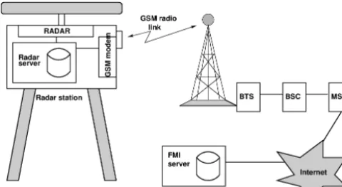
All the rasterized images are stored on the server hard disk while a subset of preprocessed images are sent to FMI. The preprocessing performed on the radar servers is a temporal median filtering of 15–20 s. The data are transmitted via a stand-alone GSM (Global System for Mobile Communica-tions) mobile link, for details see Fig. 1. Due to the limited bandwidth of the GSM modems a preprocessed image is also transmitted in every 2 min, which has proved to be a suit-able time interval for continuous ice drift monitoring. Our plans are to install the presented VB tracking software on the radar servers, leading to a reduced amount of required data transmission. In practice only VB motion, or VB motion data with radar imagery in the case of significant ice motion, then needs to be transmitted.
3 Data sets used in the study
We have used three data sets to test the new algorithm. Two of the data sets were coastal radar data from the Tankar coastal radar, located at 63.95◦N, 22.84◦E: the first data set period
Figure 1. Coastal radar and data transmission. The temporal
me-dian filtering is performed on the radar server; a PPI radar image is transmitted every 2 min by the GSM modem through the GSM base transceiver station (BTS), GSM base station controller (BSC), and mobile switching centre (MSC) and further through the Internet and to the FMI server performing the radar motion analysis.
The third data set was a longer period data set and collected on-board RV Lance during the period from 21 January 2015, 11:30 UTC, to 18 February 2015, 10:20 UTC. The time dif-ference between successive radar images of the RV Lance data set was 10 min. For demonstration purposes we selected a 1-day period (8 February 2015 from 00:00 to 24:00 UTC) of the RV Lance data set. This data set will be referred as case C here. During this time period set, significant and heteroge-neous ice motion with respect to the ship also occurred within the radar coverage. During this 1-day period the location of RV Lance was north of Svalbard, approximately 82.5◦N,
18◦E. The total range of the Tankar coastal radar data sets
was 20 km and the image size was 1200×1200 pixels; i.e. the nominal resolution was 33.3 m. For the RV Lance radar the image size in pixels was the same as for the Tankar data, but the range was only 7.5 km, resulting to a nominal reso-lution of 12.5 m. The radar image area of the Tankar radar was shifted 10 km to the west and the images were rotated 49.93◦to the counterclockwise direction on the radar server with respect to the radar location. This kind of operations can be performed on the radar server by giving the displacement and rotation parameters. The translation and rotation were performed to minimize the land area in the imagery to get a larger cover of the sea area.
To reduce radar artifacts (e.g. due to weather phenomena, radar noise or clutter, electromagnetic interference) tempo-ral median filtering in the beginning of each minute (11 im-ages, corresponding to about same amount of time in sec-onds, assuming that the radar rotation frequency is about 1 Hz) was performed. During this time period the ice mo-tion is neglectable and only the noise and possible artifacts are reduced by the filtering. The images were also processed by homomorphic filtering (HMF) to reduce the signal atten-uation as a function of the range (Lensu et al., 2014). This processing mainly makes the visual analysis of the data
eas-ier. According to some performed tests it does not have sig-nificant effect on the tracking of objects.
We also applied a rough land mask to the Tankar im-agery. Our land mask was derived from the GSHHG (Global Self-Consistent Hierarchical High-resolution Geog-raphy database) from the NOAA (National Oceanic and At-mospheric Administration) coastline data (Wessel and Smith, 1996).
For the RV Lance data we were unable to perform the tem-poral median filtering because we only had data with 10 min temporal sampling at our disposal, i.e. only one unfiltered image every 10 min.
4 Weather and ice conditions at the test sites
The air temperature on 25 February 2011 (corresponding to case A) around the Tankar lighthouse and radar station was from about−15◦C in the morning to about−3◦C in the
af-ternoon. The previous day was colder with a daily maximum temperature of about−15◦C. The wind direction was 150– 180◦, and wind speed varied in the range 6–8 m s−1. In the eastern parts of the area there was landfast ice; west of the fast ice there was a zone of very open ice (concentration 10– 30 %), and west of this zone there were very close drift ice (concentration 90–100 %). The ice thickness in the area was 20–55 cm. The ice information were extracted from the FMI ice charts.
On 8 February 2012 (case B) the air temperature around the Tankar lighthouse and radar station was from −11◦ in the morning to−20◦C in the evening; also, the previous day
the temperatures were relatively cold, below−10◦C. The
wind direction was 90–180◦, and wind speed in the range
2–6 m s−1. According to the FMI ice charts there was a fast ice zone in the eastern parts of the area, a zone of new ice to north and east of the fast ice, and very close drift ice (ice con-centration 90–100 %) further in the west. The ice thickness in the area was 5–30 cm.
On 8 February 2015 (case C) the air temperatures around RV Lance were cold, about −30◦C; the wind direction was 300–330◦ and wind speed around 8 m s−1. The ship was drifting with a speed of approximately 0.2 m s−1, first to the south and later to the southeast. According to the met.norway ice charts the ice in the area was very close drift ice (ice concentration 90–100 %), and according to the op-erational Nansen Environmental and Remote Sensing Center (NERSC) Topaz ice model (Sakov et al., 2012) the ice thick-ness was 100–120 cm in the area. As the weather was cold, the opening leads were also frozen relatively fast and the ice thickness in frozen leads was typically around 20 cm.
5 Virtual buoys and tracking algorithm
in more detail in Sect. 5.1. After this we used an edge and corner detection to locate the VBs in the first radar image of a radar image sequence and also when adding new VBs af-ter the number of VBs has reduced to a predefined level (an adjustable parameter). The tracking algorithm is also based on the optical flow (e.g. Horn and Schunck (1981) and Beau-chemin and Barron (1995)) between successive image pairs. The schematic flow diagram of our algorithm has been pre-sented in the diagram of Fig. 2. In the first phase the VBs are initialized based on features (edges and corners) detected by using absolute local binary patterns (ALBPs; described in more detail in Sect. 5.2), and then one iteration of motion tracking between the first two images of the image sequence is performed to prune the VBs due to noise amplification by the image filtering: all the images fed into the algorithm are first filtered by the HMF to reduce the range dependence of the radar signal. After this initialization a list of the auto-matically selected VBs (including the locations and cross-correlations between the matched windows) are fed to the continuous VB tracking algorithm. At each iteration a new filtered radar image is put into the tracking system and the optical flow tracking between the previous and the novel im-age is performed. After each tracking iteration the number of resulting VBs is compared to a predefined threshold (TN), and if the number of the remaining VBs is less than TN, new VBs are added starting from near range until the orig-inal number of VBs has been reached. The new VB location are defined based on ALBP features with the limitation that they are not allowed to be added closer than a given radius Rx(we have appliedRx=15 pixels here, but this parameter can be defined by the user) from the existing VBs. After the VB adding step the tracking is continued with the updated list of VBs. If still more VBs exist than the defined threshold TN, then the VB tracking is continued without updating the list of VBs.
5.1 Radar image preprocessing by HMF
The temporal median filtering is applied already on the radar server before transmitting the data. After receiving the data HMF is applied to reduce the attenuation of the signal as a function of the distance from the radar.
HMF has its background in optical image processing (Pitas and Venetsanopoulos, 1990). HMF intensityI (r, c)at image location(r, c)for an optical image is presented as a product of the illuminationLI and reflectanceRI, whereRI cab be considered as a quantity describing interesting objects in the scene andLI results from the lighting conditions, i.e.
I (r, c)=LI(r, c)RI(r, c). (1)
The applicability of the method for coastal radar imagery is readily conceived, as the images make the impression that the radar tower “illuminates” the ice field where the sea ice fea-tures reflect this “light”. To proceed, a logarithm transform is first applied to make the components of Eq. (1) additive
Figure 2. Flow diagram of the continuous VB tracking.
and linearly separable. The variations of illumination are then considered as noise that can be reduced by applying a high-pass filter. We assume that the reflectance, which is of inter-est, is represented more by the high-frequency components while the low-frequency components relate to the illumina-tion. In other words, the lighting condition is assumed to vary slowly across the image (the physical attenuation of the radar power) and reflectance is changing faster (due to deformed ice areas such as ridges). In practice the frequency filtering has here been implemented by applying the 2-D fast Fourier transform (FFT) to the image, then performing the high-pass filtering in the Fourier domain, and finally performing the in-verse FFT. Because FFT requires the size of the input to be a power of 2, we extend our image to the nearest power of 2 larger than the image size by mirroring with respect to the im-age boundaries (in our case a 1200×1200 pixel image is ex-tended to 2048×2048 pixel image). In the frequency (FFT) domain the low-pass coefficients are attenuated by multiply-ing by a factorf <1.0; in our case we have usedf =0.0, i.e. totally zeroing the low-frequency components. A schematic presentation of the HMF principle is shown in Fig. 3. An ex-ample of HMF for a radar image of the case. A time series is shown in Fig. 4.
5.2 Local binary patterns and VB selection
tex-Figure 3. The principle of homomorphic filtering. A logarithmic
transform is applied to make the illumination and reflection terms additive, a high-pass filter is then applied, and an exponential trans-form is applied to invert the log transtrans-form.
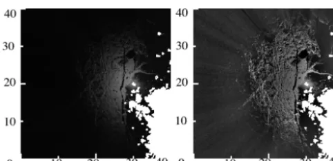
Figure 4. One temporal median filtered radar image (25 February
2011, left) and the same image after the homomorphic filtering. The land areas according to our rough land mask are masked off (white area in the figures). The associated scale is in kilometres.
ture measure or for detecting certain imagery features such as edges and corners. We used a step of5/4 in direction cor-responding to 8 bit binary patterns; the radiusRLBP(distance
from the centre pixel, see Fig. 5) used here was 2. A (8 bit) local binary pattern is defined as
LBP=
7
X
k=0
s1(gk−gc)2k, (2)
wheregcis the grey tone of the centre pixel and the values of
gk are the grey tones in the 8 pixels within the given radius RLBParound the centre pixel (see Fig. 5) ands1(x)defined
as
s1(x)=
(
1, ifx≥0
0, ifx <0. (3)
Herexis a generic argument fors1; for LBP,x=gk−gc. We have used a variant which we here call the ALBP:
ALBP=
7
X
k=0
s2(gk−gc)2k, (4)
ands2(x)defined as
s2(x)=
(
1, if|x| ≥T
0, if|x|< T . (5)
T is a threshold value and we have used value T =10 in this study. Rotational invariance can be achieved by using the minimum among all the (eight) cyclic shifts of the ALBP.
Figure 5. Geometry of an LBP with an angular step of5/4. The circle has a radius ofR, which is one LBP parameter.
This is denoted here by ALBPr. The value 15 of ALBPr
cor-responds to an edge point, value 31 corcor-responds to a corner point, and value 63 corresponds to a sharp corner point. The ALBP 15 corresponds to the pattern of four adjacent points Gi(i=0. . .7) with the value of 1 (see Fig. 5), 31 to a pattern of five adjacent pointsGi with the value of 1, value 63 to a pattern of six adjacent points with a value of 1, and all the other valuesGiof 0.
We also first locate all the corner and sharp corner points over the radar image and, based on the local densities of corner and sharp corner points, search for suitable objects for VBs. The idea is to select such areas of the radar im-age where there are many corner and sharp corner points, i.e. local maxima of their densities. The corners are searched to locate locally unique features containing nonlinear edges, because linear edges often are similar along the edge and can lead to similarization errors in the tracking process.
We select the points which locally (within a given radius Rb) maximize the complexity functionFc:
Fc(r, c)=Nc(r, c, Rs)Nsc(r, c, Rs), (6)
where Nc(r, c, Rs) is the number of corner points within
a search radiusRsfrom the location described by the column
and row coordinates(r, c), andNsc(r, c, Rs)is the number of
sharp corner points within the same area. To avoid assign-ing VBs too close to each other, we only perform the search Rs or more outside the already assigned VB locations. We
have used valuesRb=30 andRs=15 pixels here, but these
parameters can be defined by the user.
Because we apply the HMF prior to the VB selection, we also get relatively many VBs in the far range, because the filtering also amplifies the noise in the far range. For this reason, to properly initialize the VBs we perform one VB tracking iteration between the first and second images of the sequence to remove the VBs due to this noise amplification. This first iteration removes the VBs generated by random fluctuation (amplified radar noise).
In the areas of no distinguishable ice features (low signal-to-noise ratio) in the imagery the tracking can not be reliably performed. For example in the far radar range this is typically the case. Typically there are enough ice features available and suitable for tracking ice drift in the drift ice field; within drift ice deformation continuously occurs, leading to ice features visible in radar (e.g. ice ridges). The algorithm only adds and tracks VBs in the areas where such traceable targets exist. 5.3 Optical flow and algorithm implementation
Optical flow (Horn and Schunck, 1981; Beauchemin and Barron, 1995) is a method used for estimating motion in im-age sequences such as in digital video. In optical flow we assume an intensity at a location (x, y) in a digital image at time to be moving such that
I (x, y, t )=I (x+1x, y+1y, t+1t ). (7) Using the Taylor expansion and assuming small motion, I (x+1x, y+1y, t+1t )=I (x, y, t )+δI
δx1x
+δI δy1y+
δI
δt1t+HOT ⇒δI
δx1x+ δI δy1y+
δI
δt1t=0, (8)
where HOT stands for higher-than-first-order terms. Divid-ing by1twe get the optical flow equation:
Ixvx+Iyvy= −It, (9)
where Ix, Iy, and It indicate the partial derivatives of the image signal with respect to x,y, andt. The changes ofI at (x, y) inx andy directions and change ofI in time can be estimated from an image pair. To perform the estimation additional conditions are needed. One practical approach is the Lucas–Kanade method (Lucas and Kanade, 1981) where it is assumed that optical flow equation holds for a block of N pixelspk (k=1, . . ., N):
Ix(p1)vx+Iy(p1)vy= −It(p1)
. . . (10)
Ix(pN)vx+Iy(pN)vy= −It(pN).
This corresponds to a (overdetermined) linear systemAv= b, wherev= [vx vy]T and
A=
Ix(p1) Iy(p1)
. . .
Ix(pN) Iy(pN)
(11)
and
b=
−It(p1)
. . . −It(pN)
. (12)
The block of N pixels consists of pixels within a round-shaped window around a centre pixel (VB centre). This lin-ear overdetermined system of equations can be solved (least squares solution) (Penrose, 1955) as
v=(ATA)−1ATb=Mb. (13)
M=(ATA)−1AT is known as the Moore–Penrose pseu-doinverse.
We have used the following discrete estimates forIx,Iy, andIt (Horn and Schunck, 1981):
Ix=(I1(r+1, c)−I1(r, c)+I1(r+1, c+1)
−I1(r, c+1)+I2(r+1, c)−I2(r, c)
+I2(r+1, c+1)−I2(r, c+1))/4
Iy=(I1(r, c+1)−I1(r, c)+I1(r+1, c+1)
−I1(r+1, c)+I2(r, c+1)−I2(r, c)
+I2(r+1, c+1)−I2(r+1, c))/4
It=(I2(r, c)−I1(r, c)+I2(r+1, c)−I1(r+1, c)
+I2(r, c+1)−I1(r, c+1)+I2(r+1, c+1)
−I1(r+1, c+1))/4, (14)
whereI1andI2are the first and second (in this temporal
or-der) image of an image pair, and (r, c) refers to the row and column coordinates which are used here instead ofx andy. The image pixel values with fractional coordinates are com-puted using bilinear interpolation. For numerical stability it is essential that the estimates forIx,Iy, andIt are computed at the same spatiotemporal location.
The optical flow method is best suitable for short mo-tion corresponding to short time differences, e.g. for our coastal radar data with a relatively short time difference (in our case 2 min). In practice some image smoothing at sharp edges is recommendable before the optical flow computa-tion, because optical flow assumes continuity of the signal. For this reason we perform a spatial Gaussian smoothing of the images before the optical flow estimation. The Gaussian smoothing is combined with the original image data by a lin-ear combination to get the smoothed pixel valueI0(r, c)from the original pixel valueI (r, c)and the smoothed pixel value G(r, c)(Grefers to the image convolved with a predefined Gaussian kernel):
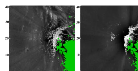
Figure 6. The initial VBs of the February 2011 test data set (a), and
the February 2012 data set (b) drawn over the first radar images of the sequences. The coordinates are in kilometres, and the radar is located at (row, column)=(20,30). The land area according to our rough land mask is indicated in green. The associated scale is in kilometres.
and the smoothed pixel value a weight of 0.8 in the linear combination used.
In computation of the optical flow we used a spherical win-dow with a radius of 11 pixels (resulting toN=377 pixels involved) for the coastal radar data and a a spherical window with radius of 21 pixels (N=1373) for the ship radar (with longer time difference between the successive images) in the optical flow estimation.
If the cross-correlation between two matched windows is less than a given thresholdTccthe object is not tracked any
more, i.e. the VB is lost. We have usedTcc=0.9 in our
ex-periments presented here. We also studied the use of the co-efficient of determination of the linear fits as a measure of the matching quality, but it seems to have insignificant corre-lation e.g. with respect to the cross-correcorre-lation, which seems to be a more useful measure. The first tracking iteration (be-tween the first and second images) is used to prune the unre-liable VBs produced by noise amplification due to the HMF. The same cross-correlation thresholding is applied for this purpose.
6 Experimental results
6.1 Coastal radar image sequences
The initial radar images (first images in the image sequences) of the two coastal radar image sequences of cases A and B, with the locations of the initial VBs indicated, used in our experiments are shown in Fig. 6. The location of the radar indicated by the green dot and the initial VBs are indicated by red dots and the location of the radar by green dots.
The first and last images of case A and case B are shown in Figs. 7 and 8 respectively. From these images we can see the change of the ice field during the whole study period. In case A a large ice field is torn off and drifting away from the land and landfast ice zone. In case B a smaller part of
Figure 7. The first and last image of the February 2011 test data set.
The coordinates are in kilometres, and the radar is located at (row, column)=(20,30). The land area according to our rough land mask is indicated in green. The associated scale is in kilometres.
Figure 8. The first and last image of the February 2012 test data set.
The coordinates are in kilometres, and the radar is located at (row, column)=(20,30). The land area according to our rough land mask is indicated in green. The associated scale is in kilometres.
the ice is also torn off and floating away from the coast. The trajectories resulting from the Lucas–Kanade optical flow al-gorithm for the two test cases are shown in Fig. 9a and b. We can see that for case A the direction of the motion was rather uniform over the whole drift ice area, but for case B the di-rection of the motion was less uniform. However, this kind of trajectory plots do not show the ice drift velocity evaluation as a function of time.
Figure 9. Trajectories of the VBs which survived the whole
Febru-ary 2011 and FebruFebru-ary 2012 test periods. The three VBs whose properties are studied in more detail in both the cases are indicated in red. The starting point of a trajectory is indicated by an open circle and the end point by a closed circle. The coordinates are in kilometres, and the radar is located at (row, column)=(20,30). The land area according to our rough land mask is indicated in green. The associated scale is in kilometres.
For case A a large part of the ice was torn off the fast ice and drifting to north/northwest (Figs. 7 and 9a). For this case we applied a thresholdTN=75 % of the original number of VBs. The number of VBs as a function of time for this case is shown in Fig. 10a. We adjustedTN this high just to demon-strate the adding of VBs, in practice a lower value could be used. For case B some smaller ice floes were torn off and drifting to the northwest and west (Figs. 8 and 9b). For this case we usedTN=90 % of the original number of VBs. The number of VBs as a function of time is shown in Fig. 10b. Because the total time was longer for this case the VBs were added twice during the whole time period of 24 h.
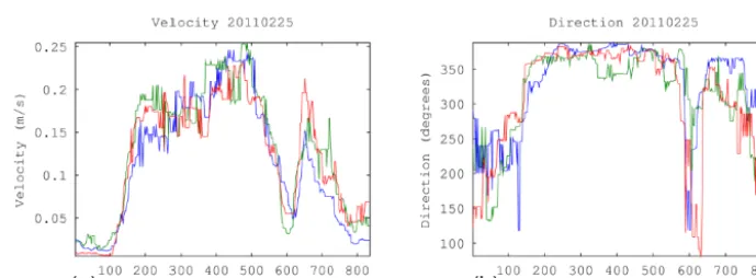
It is also straightforward to compute the velocity and direc-tion (here given as the compass direcdirec-tion with 0◦to the north, 90◦to east, and so on) by just dividing the displacement con-verted to metres by the time step of 2 min for each successive image pair. The velocities and direction for the selected three VBs of case A are shown in Fig. 11. It can be seen that the three VBs are moving rather coherently. The velocity is first very slow and the direction rather ambiguous. Then the ve-locity is accelerated rather rapidly (the average acceleration a can be estimated by dividing the velocity differences be-tween the two adjacent velocities by the length of the time step: a≈3.0×10⁻⁵m s−2). It can also be seen that as the direction changes for a short time, the velocity is reduced (around time 600 min). In Fig. 12 the velocity and direction are shown for case B. Also in this case the ice is quite stable for a while in the beginning of the time period and then the velocity accelerates (in the beginning,a≈1.5×10⁻⁵m s−2; later the average acceleration in general is lower but exhibits temporal variation) to a top value of about 0.3 m s−1achieved near the end of the period. For case A the top velocity was a little lower and achieved about in the middle of the time period. For case B the velocities of the three studied VBs
were less uniform than for case B. This also results to the larger divergence for this case compared to 25 February 2011 case. The ratio of the area of a triangle formed by a selected triplet of points to the area of the triangle formed by the same triplet in the beginning of the study time period are shown in Fig. 13 for the cases A and B. These figures indicate the local ice convergence (decreasing value) or divergence (increasing value).
For case A we can see divergence after the motion starts (after around 100 min) to around 300 min, and then about 100 min of convergence and then divergence again. The di-vergence is increased around 600 min, and finally after about 700 min the VBs move uniformly for the rest of the time. The VB velocity accelerates from 0 to about 0.2 m s−1during the period from approximately 100 to 300 min; also during this period the relative area increases, indicating divergence. Dur-ing the period from approximately 300 to 400 min the VB velocity remains about similar, but there is some variability in the velocities and directions of the single VBs leading to convergence during this period. After this, during the time period from about 400 to 600 min, the VBs move quite uni-formly while their velocity first increases and then decreases. After 600 min the velocity of all the VBs accelerates from about 0.05 m s−1to about 0.2 m s−1 and during this period we also see differences in the velocity of the different VBs and due to these differences also the relative area increases (indicating divergence).
For case B, there is a period of divergence from about 200 min to about 800 min, and after that the VBs move quite uniformly to the end of the period. During the diverging pe-riod, there seem to be one VB (the northernmost one) moving faster than the two other VBs, mostly explaining the diver-gence. The relative area changes were from 1.0 to 1.2 for case A and from 1.0 to 1.5 for case B. In case B the ice con-centration in later parts of the period was quite low, but in case A the VBs were part of a larger drifting ice field.
ac-Figure 10. Number of VBs at each time step for the 2011 case (a) and for the 2012 case (b). The threshold to add new VBs was 75 and 90 %
of the original number of VBs respectively.
Figure 11. Velocity (a) and direction (b) for the 2011 case selected three VBs. The direction is in degrees.
cordance with the free drift model ice direction, taking into account that the Finnish coastline in the east was restricting the eastward drift component.
For case B the wind speed was approximately in the range 4–6 m s−1during the first 8 h of the study period. During the second 8 h period the wind speed was in the range 2–4 m s−1, and during the last 8 h period it increased to approximately to 4–5 m s−1. The wind direction during the period varied from about 180◦ to about 90◦ and then back to about 150◦. Ac-cording to the free drift model the ice drift velocities in the three 8 h periods would have been approximately 0.12, 0.08, and 0.11 m s−1. There was, just like in case A, a static period in the beginning of the study period, but after the ice motion started the VB velocities were somewhat larger than the val-ues based on the free drift model. One reason for this may be that the ice was relatively thin and drift ice concentration was low as the ice proceeded faster further from the coast. The ice drift direction of Fig. 12b corresponded to the free drift model quite well.
6.2 Ship radar image sequence
The RV Lance ship radar data were collected during the pe-riod from 21 January to 18 February, and the temporal dif-ference between each image pair was 10 min, which is quite long for an optical flow algorithm. The ship was drifting in
ice and no ship motion correction based on ship GPS has been performed; i.e. the detected ice drift is the drift with respect to the ship. The ship motion could be compensated based on the ship GPS, but we did not have this information available when this study was performed.
We computed the tracking for the whole period but here we only show the results for a 1-day period with some in-teresting motion. During many of the days the motion with respect to the ship was not significant. Because the ship radar had a shorter range and higher resolution there were sea ice details visible over the whole image.
Figure 12. Velocity (a) and direction (b) for the 2012 case selected three VBs. The direction is in degrees.
Figure 13. Ratio of the area of the triangle formed by the selected three VBs with respect to the area in the beginning of the period for the
2011 case (a) and for the 2012 case (b).
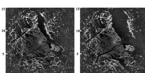
Figure 14. The first and last radar images of the RV Lance 1-day
test period. The ship radar is located in the middle of the image. The associated scale is in kilometres.
are shown in Figs. 16 and 17. In this case the direction changes quite suddenly around the 300–400 min mark. How-ever, there is no significant reduction in the computed drift velocity. This may be due to the relatively sparse time step of 10 min; with 2 min time steps the observed speed change might have been larger. It can also be seen that some con-vergence occurs for the ice area described by the selected triplet of VBs. The area is decreased to about 80 % of the original area. This is because the VBs belong to the ice field east of the opening lead and the ice is converging in this
Figure 15. Trajectories of the VBs which survived the RV Lance
1-day February 2015 test periods. The three VBs whose properties are studied in more detail in both cases are indicated in red. The starting point of a trajectory is indicated by an open circle and the end point by a closed circle. The associated scale is in kilometres.
Figure 16. Velocity (a) and direction (b) for the RV Lance 2015 case selected three VBs. The direction is in degrees.
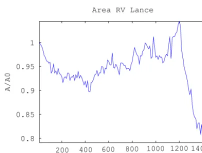
Figure 17. Ratio of the area of the triangle formed by the selected
three VBs with respect to the area in the beginning of the period for the 2015 RV Lance case.
For case C, the wind direction also varied in the range 300–330◦, and wind speed was around 8 m s−1. According
to the free drift model this would result in drift direction of about 90–120◦and speed around 0.015 m s−1. These values
approximately correspond to the ship drift speed and direc-tion. As the VB drift was estimated with respect to the ship we were not able to apply the free drift model to the estimated VB velocity and direction of Fig. 16. We can see that in the beginning as the ice drift with respect to the ship is slow the ice drift direction is approximately the same as the ship drift direction (ice is moving slightly faster than the ship to ap-proximately same direction), but after the non-homogeneous dynamic ice drift events begin there are some relatively rapid changes in the VB velocities and directions. These relative changes were due to the local surface current and wind de-viations. The compression in the triangle described by the triplet of VBs started around 1200 min and continued to the end of the period. During this period the velocity also de-creased proportionally to the decrease of the triangle area. This is also an expected result as the ice velocity tends to reduce in compressing ice.
6.3 Evaluation of the estimation error
We performed a study in which we compared some visu-ally selected points within some target windows (VB area) of a moving VB and manually defined the location after each 200 min steps (100 2 min time steps) in the four Tankar coastal radar VB sets. The selected points were not neces-sarily in the middle of the window (which corresponds the VB location in the algorithm), but such points which could be visually located in the time series of radar images. If we assume that the VB area remains unchanged (acts as a rigid object) then the difference between the VB centre and the studied point should remain constant. We computed the stan-dard deviation of the difference for our selected points and the VB centres for the row and column coordinates and got valuesσr =1.41 and σc=1.24. The manually defined lo-cations were always integers; i.e. the lolo-cations were defined visually from the image by pointing the pixel by a mouse and recording the pixel coordinates with a precision of one pixel. There are three sources of error in the manual estimation: hu-man estimation error, rounding error to an integer pixel (on average 0.25 pixels in both directions), and changes due to possible internal transformations within the VB area. Based on this analysis we can only estimate the error in VB posi-tion to roughly be less than or equal to 1 pixel (33 m) in both coordinate directions, because it is difficult to estimate the exact contributions of the error sources present.
In Fig. 18 we show the locations of the VBs (red) and lo-cations of the manually tracked points within the VB area for one case A time series. Also the corresponding VB and some ice area around it at the time instants 0, 200, 400, 600, and 800 min are shown in the figure. A thorough evaluation using this method would in practice be labour intensive. An estima-tion error of roughly 1 pixel in both coordinate direcestima-tions in 2 min seems to overestimate the actual error; in addition, we also studied other methods of estimating the error.
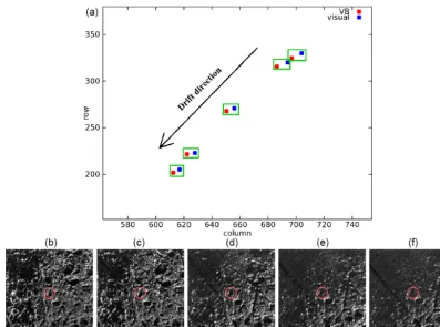
se-Figure 18. An example of manual VB pixel location estimation and VB location defined by the algorithm with a time step of 200 min (case
A). The locations are shown in (a): the red dots indicate the VB centre location, the blue dots the selected and tracked feature location, and the corresponding pairs have been marked with the green rectangles. The VB areas (red circles) in the radar imagery with some background included at the given time instants are shown in time order from left to right in (b)–(f).
ries and computed the means and standard deviations of the successive (with a time difference of 2 min) location differ-ences ofrandccoordinates (row and column) for three VBs of this time series. We got for the valuesµ1r= −0.020 and µ1c= −0.035 for the means and σ1r=0.126, and σ1c= 0.120 Tankar radar pixels (33 m) for the standard deviations. We also performed a similar study with the RV Lance case by selecting a VB which was visually static during the whole 1-day study period and computed the valuesµ1r= −0.00076 andµ1c= −0.000393 for the means andσ1r=0.145, and σ1c=0.142 RV Lance radar pixels (12.5 m). The standard deviations can be considered as estimates of the location esti-mation error in the row and column directions. Possibly there still were some minor ice motion (not easily visible by eye) in the Tankar radar case as the values ofµ1randµ1c were significantly higher than for the RV Lance data.
For comparison, the error of GPS is 15m or less for 95 % of the time (Hofmann-Wellenhof et al., 2008). Some addi-tional error in the GPS location is caused by the water level changes. This gives an idea of the location error of buoys equipped with GPS positioning.
The accuracy of the derived quantities such as velocity, direction, and area of a triangle formed by three VBs can be estimated based on the multivariate Taylor expansion; if
we assume the errors are relatively small, we can also as-sume the higher-order terms to be neglectable and estimate the error by the first-order terms. If the derived quantityZ is a function of the original quantitiesXi,i=1, . . ., n, i.e. Z=F (X1, . . ., Xn), then the error1U at(X1, . . ., Xn)can be estimated as, see e.g. (Steward, 1996),
1U= n X
i=1
∂F ∂Xi
1Xi. (16)
We can compute the error estimates for the velocity v and direction θ from their formulas v=s/t, and θ= arctan(dr/dc), where s is the drift of the VB between the 2 or 10 min time period,t is the time (2 or 10 min), dr is the row direction drift, and dc is the column direction drift within a given time period. Also the corresponding error estimate for the triangle areaAcan be estimated based on the equation used for the triangle areaA:
A= |(r1(c2−c3)+r2(c3−c1)+r3(c1−c2)|/2, (17)
where(r1, c1),(r2, c2), and(r3, c3)are the corner row and
is neglectable, we get the estimates 1v≈0.05 m s−1 for the Tankar cases (A and B) and 1v≈0.004 m s−1 for the RV Lance case (C). The derived error estimation formula for the ice drift direction has the ratios of dr2+dc2in the denom-inator, and for this reason it will give unreliable estimates for small values of drift in the case both dr and dc are small. According to our experiments the estimates of the direction are not very reliable (include a lot of variation) for veloci-ties lower than approximately 0.1 m s−1. This can be seen in Figs. 11b and 12b in the beginning of the two periods as the ice motion is small, or does not exist at all, as large varia-tions of the direction estimates. According to our evaluation the relative error in the computed triangle (formed by VB triplets) size is about 0.5–0.6 % of the triangle area for case A, 0.8–1.1 % for case B, and 1.3–1.5 % for case C.
7 Discussion and conclusions
An algorithm for ice tracking was developed to track virtual ice buoys. The algorithm enables continuous ice drift track-ing by addtrack-ing VBs after a certain absolute or relative amount of VBs has been lost; this number or ratio can be defined by the algorithm user. The location of the VBs are initialized automatically based on the local information content of the image favouring locations with well-distinguishable features. The VBs can also be initialized manually if some specific case studies are made. This method is best suitable for rel-atively short temporal steps and giving sub-pixel resolution, unlike our earlier algorithm based on cross-correlation (Kar-vonen, 2013a). From the VB tracks many kinds of derived quantities, such as divergence, shear, vorticity, and total de-formation, can be computed and information on the nature of the ice dynamics extracted. For example it is possible to dis-tinguish between deformed ice and level ice or open water at least in the near range area, and opening of new open water channels can also be identified.
The main advantages of this algorithm are the capabil-ity of sub-pixel resolution and capabilcapabil-ity to monitor sea ice alone and continuously by adding VBs when needed. The estimation cannot be performed in the areas where no distin-guishable ice features are present in the radar imagery. How-ever, usually there are such features available in the radar im-ages of drift ice and VB tracking is possible. Also the imag-ing geometry imposes some restrictions, especially in the far range. The typical ice ridges in the Baltic are at maximum several metres high and are not very well visible in the far range as their backscattering towards radar is less than that of larger (higher) targets. However, their shadowing effect is also less, even though for example a typical 2 m high ridge has a shadow of approximately 1 km in the range of 15 km, assuming the radar to be at a 30 m altitude from the sea sur-face and (locally) flat earth geometry. This may reduce the number of targets suitable for a VB in the far range.
The lost targets were typically lost as they had drifted away from the radar and signal-to-noise ratio had become lower. In general the number of traceable targets depends on the density of good scatterers (deformed ice, e.g. ridges) within the radar range. The algorithm radius parameters have been selected such that adjacent VBs are not very close to each other. If there are images of poor quality in the radar image sequence, e.g. due to weather conditions or radio-frequency signal interference from other sources (e.g. other radars), more VBs can be lost and the tracking can temporally be interrupted, but it will be restarted (by adding new VBs) as soon as the radar image quality has recovered.
We applied the developed algorithm to three test cases. Here we only computed some relatively simple derived quan-tities related to the ice dynamics, i.e. velocity, direction, and the relative area defined by triplets of VBs. The relative VB triplet areas give information on the divergence and conver-gence of the ice and also to some degree on the compres-sion in the ice. Some other and more sophisticated ways to analyse VB data have been presented e.g. in Karvonen et al. (2013). The main purpose of this study was the development and testing of the VB tracking system.
The VB drift results for the test cases were evaluated based on visual inspection of the animations of the image sequences with overlaid VB positions. There were no real buoy data available. The visual analysis showed that the al-gorithm results correspond to the visual interpretation and same targets were tracked throughout the radar image se-quences. This could also be visually verified by extracting single frames of the radar image time series with a time dif-ference of e.g. 2–3 h and with some given VB positions indi-cated on the radar images. Also, according to this verification the algorithm tracking results and visual inspection were in good agreement. Also some attempts to estimate the estima-tion error numerically were made for the test cases.
This VB tracking software complemented some basic VB data analysis software tools will be included in the radar servers, making automated ice dynamics analysis in real time or near-real time possible. The analysis tools will include the analysis of VB drift velocity and direction as well as di-vergence based on triangles formed by VB triplets. These will be computed within the convex polygon defined by the outer VBs in the image in a given grid and for a given time step (multiple of the basic time step). This integration is un-der construction as part of the project “Harnessing Coastal Radars for Environmental Monitoring Purposes” (HARD-CORE) funded by the Baltic Sea Research and Development Programme (BONUS).
Acknowledgements. The author would like to thank Norwegian
Polar Institute (NPI) and Jari Haapala (FMI) for providing the RV Lance data for this study.
References
Beauchemin, S. S. and Barron, J. L.: The Computation of Optical Flow, ACM Computing Survey v. 27, n. 3, 433–467, 1995. Cohen, M. N.: Principles of Modern Radar Systems, Chapman and
Hall, New York, USA, 465–501, 1987.
Druckenmiller, M. L., Eicken, H., Johnson, M. A., Pringle, D. J., and Williams, C. C.: Toward an integrated coastal sea-ice obser-vatory: System components and a case study at Barrow, Alaska, Cold Reg. Sci. Technol., 56, 61–72, 2009.
Fily, M. and Rothrock, D. A.: Sea ice tracking by nested correla-tions, IEEE T. Geosci. Remote, 5, GE-25, 570–580, 1987. Haarpaintner, J.: Arctic-wide operational sea ice drift from
enhanced-resolution QuikScat/SeaWinds scatterometry and its validation, IEEE T. Geosci. Remote, 44, 102–107, 2006. Harris, C. and Stephens, M.: A combined corner and edge
detec-tor, Proc. of Alvey Vision Conference, Univ. of Manchester, 31 August–2 September 1988, Manchester, UK, 147–151, 1988. Hofmann-Wellenhof, B., Lichtenegger, H., and Wasle, E.: GNSS –
Global Navigation Satellite System, Chapter 9 (GPS), Springer, Wien/NewYork, 309–340, 2008.
Horn, B. K. P. and Schunck, B. G.: Determining optical flow, Artif. Intell., 17, 185–203, 1981.
Image Soft: Radar Recording Server, Technical Manual, version 2014.09.0, Image Soft Ltd, Finland, 2014.
Jones, J. M.: Landfast sea ice formation and deformation near Bar-row, Alaska : variability and implications for ice stability, 80 pp., University of Alaska Fairbanks, Fairbanks, AK, USA, 2013. Karvonen, J.: Operational SAR-based sea ice drift monitoring over
the Baltic Sea, Ocean Sci., 8, 473–483, doi:10.5194/os-8-473-2012, 2012.
Karvonen, J.: Tracking the motion of recognizable sea-ice objects from coastal radar image sequences, Ann. Glaciol., 54, 4149 pp., 2013.
Karvonen, J., Heiler, I., Haapala, J., and Lehtiranta, J.: Ice objects tracked from coastal radar image sequences as virtual ice buoys, Proc. of The International Conferences on Port and Ocean En-gineering under Arctic Conditions (POAC’13), abstract number POAC13_030, 9–13 June 2013, Espoo, Finland, 2013.
Kwok, R., Curlander, J. C., McConnell, R., and Pang, S. S.: An Ice-Motion Tracking System at the Alaske SAR Facility, IEEE J. Oceanic Eng., 15, 44–54, 1990.
Lensu, M., Heiler, I., and Karvonen, J.: Range compensation in pack ice imagery retrieved by coastal radars, in: Proc. IEEE Baltic In-ternational Symposium (BALTIC), 27–29 May 2014, Tallinn, Es-tonia, 1–5, 2014.
Lepparanta M.: The Drift of Sea Ice, 2nd edition, p. 143, Praxis publishing, Chichester, UK, 2009.
Lepparanta, M. and Myrberg, K.: Physical Oceanography of the Baltic Sea, p. 252, Praxis publishing, Chichester, UK, 2009. Lucas, B. and Kanade, T.: An iterative image registration technique
with an application to stereo vision, in: Proceedings of the 7th International Joint Conference on Artificial Intelligence (IJCAI), 24–28 August 1981, Vancouver, Canada, vol. 2, 674–679, 1981. Mahoney, A., Eicken, H., and Shapiro, L.: How fast is landfast sea ice? A study of the attachment and detachment of nearshore ice at Barrow, Alaska, Cold Reg. Sci. Technol., 47, 233–255, 2007.
Mahoney, A. R., Eicken, H., Fukamachi, Y., Ohshima, K. I., Simizu, D., Kambhamettu, C., Mv, R., Hendricks, S., and Jones, J.: Tak-ing a look at both sides of the ice: comparison of ice thickness and drift speed as observed from moored, airborne and shore-based instruments near Barrow, Alaska, Ann. Glaciol., 56, 363– 372, 2015.
MV, R., Jones, J., Eicken, H., and Kambhamettu, C.: Extracting quantitative information on coastal ice dynamics and ice hazard events from marine radar digital imagery, IEEE T. Geosci. Re-mote, 51, 2556–2570, 2013.
Ojala, T., Pietikainen, M., and Harwood, D.: A comparative study of texture measures with classification based on feature distribu-tions, Pattern Recogn., 29, 51–59, 1996.
Penrose, R.: A generalized inverse for matrices, P. Camb. Philos. Soc., 51, 406–413, doi:10.1017/S0305004100030401, 1955. Peura, M. and Hohti, H.: Optical flow in radar images, in: Proc.
Third European Conference on Radar in Meteorology and Hy-drology (ERAD2004), Copernicus, 454–458, 6–10 September 2004, Visby, Sweden, 2004.
Pitas, I. and Venetsanopoulos, A. N.: Nonlinear Digital Filters, Prin-ciples and Applications, Chapter 7 “Homomorphic Filters”, 217– 243, Springer, New York, ISBN: 978-1-4419-5120-5, 1990. Sakov, P., Counillon, F., Bertino, L., Lisæter, K. A., Oke, P. R., and
Korablev, A.: TOPAZ4: an ocean-sea ice data assimilation sys-tem for the North Atlantic and Arctic, Ocean Sci., 8, 633–656, doi:10.5194/os-8-633-2012, 2012.
Shapiro, L. H.: A preliminary study of ridging in landfast ice at Barrow, Alaska, using radar data, paper presented at 3rd Inter-national Conference on Port and Ocean Engineering under Arc-tic Conditions (POAC), University of Alaska, Fairbanks, Alaska, 417–425, 1976.
Shapiro, L. H. and Metzner, R.: Nearshore ice conditions from radar data, Point Barrow, AlaskaUAG R-268, 46 pp., Geophysical In-stitute, University of Alaska Fairbanks, 1989.
Stewart, J.: Multivariable Calculus, 3rd Edition, Brooks/Cole Pub-lishing Company, Pacific Grove, CA, USA, p. 790, 1995. Sun, Y.: A new correlation technique for ice-motion analysis,
EARSeL Adv. Remote Sens., 3, 57–63, 1994.
Tabata, T., Kawamura, T., and Aota, M.: Divergence and rotation of an ice field off Okhotsk Sea Coast of Hokkaido, annals of glaciol-ogy, in: Sea Ice Processes and Models, edited by: Pritchard, R. S., University of Washington Press, Seattle, USA, 273–282, 1980. Thomas, M., Geiger, C., and Kambhamettu, C.: Discontinuous
non-rigid motion analysis of sea ice using C-band synthetic aper-ture radar satellite imagery, IEEE Workshop on Articulated and Nonrigid Motion (ANM, In conjunction with IEEE CVPR’04), 27 June–2 July 2004, Washington DC, USA, available at: http: //vims.cis.udel.edu/publications/anm-thomas.pdf (last access: 21 October 2015), 2004.
Thomas, M., Geiger, C. A., and Kambhamettu, C., High resolution (400 m) motion characterization of sea ice using ERS-1 SAR im-agery, Cold Reg. Sci. Technol., 52, 207–223, 2008.