www.ocean-sci.net/13/175/2017/ doi:10.5194/os-13-175-2017
© Author(s) 2017. CC Attribution 3.0 License.
Characteristics and causes of Deep Western Boundary Current
transport variability at 34.5
◦
S during 2009–2014
Christopher S. Meinen1, Silvia L. Garzoli2,1, Renellys C. Perez2,1, Edmo Campos3,2, Alberto R. Piola4,5,6, Maria Paz Chidichimo4,5,6, Shenfu Dong1, and Olga T. Sato3
1Physical Oceanography Division, Atlantic Oceanographic and Meteorological Laboratory, Miami, Florida, USA 2Cooperative Institute for Marine and Atmospheric Studies, University of Miami, Miami, Florida, USA
3Instituto Oceanográfico, University of São Paulo, São Paulo, Brazil
4Departamento Oceanografia, Servicio de Hidrografía Naval, Buenos Aires, Argentina 5Departamento Oceanografia, Universidad de Buenos Aires, Buenos Aires, Argentina
6Instituto Franco-Argentino sobre Estudios de Clima y sus Impactos, Consejo Nacional de Investigaciones
Científicas y Técnicas (CONICET), Argentina
Correspondence to:Christopher S. Meinen ([email protected]) Received: 26 September 2016 – Discussion started: 17 October 2016
Revised: 23 January 2017 – Accepted: 13 February 2017 – Published: 2 March 2017
Abstract. The Deep Western Boundary Current (DWBC)
at 34.5◦S in the South Atlantic carries a significant frac-tion of the cold deep limb of the Meridional Overturning Circulation (MOC), and therefore its variability affects the meridional heat transport and consequently the regional and global climate. Nearly 6 years of observations from a line of pressure-equipped inverted echo sounders (PIESs) have yielded an unprecedented data set for studying the char-acteristics of the time-varying DWBC volume transport at 34.5◦S. Furthermore, the horizontal resolution of the ob-serving array was greatly improved in December 2012 with the addition of two current-and-pressure-equipped inverted echo sounders (CPIESs) at the midpoints of the two west-ernmost pairs of PIES moorings. Regular hydrographic sec-tions along the PIES/CPIES line confirm the presence of recently ventilated North Atlantic Deep Water carried by the DWBC. The time-mean absolute geostrophic transport integrated within the DWBC layer, defined between 800– 4800 dbar and within longitude bounds of 51.5 to 44.5◦W, is−15 Sv (1 Sv=106m3s−1; negative indicates southward flow). The observed peak-to-peak range in volume transport using these integration limits is from−89 to+50 Sv, and the temporal standard deviation is 23 Sv. Testing different verti-cal integration limits based on time-mean water-mass prop-erty levels yields small changes to these values, but no sig-nificant alteration to the character of the transport time
se-ries. The time-mean southward DWBC flow at this latitude is confined west of 49.5◦W, with recirculations dominating the flow further offshore. As with other latitudes where the DWBC has been observed for multiple years, the time vari-ability greatly exceeds the time mean, suggesting the pres-ence of strong coherent vortices and/or Rossby Wave-like signals propagating to the boundary from the interior.
1 Introduction
under-stood as in the North Atlantic. In a recent paper, Garzoli et al. (2015) used all available WOCE and CLIVAR-era hydro-graphic sections including dissolved oxygen and chloroflu-orocarbon (CFC) data, Argo float profile data, and two dif-ferent analyses of the Ocean General Circulation Model For the Earth Simulator (OFES) to trace the time-mean pathways of the DWBC through the South Atlantic. Together with other historical analyses, their results show that the DWBC crosses 5◦S as a narrow western boundary current, and it becomes dominated by eddies further south around 8–11◦S, consistent with earlier mooring observations (Dengler et al., 2004; Schott et al., 2005). Previous work has suggested that when this very energetic eddying flow reaches the Vitória-Trindade Ridge at about 20◦S, the mean flow appears to fol-low two different pathways, with a significant fraction (es-timates ranging from 3 to 12 Sv) flowing eastward across the Mid-Atlantic Ridge toward the African continent (e.g., Zangenberg and Siedler, 1998; Arhan et al., 2003; Hogg and Thurnherr, 2005; van Sebille et al., 2012) and the remain-der flowing southward along the western boundary hugging the South American continental slope. The recent analysis of ship sections of CFC, oxygen, and salinity by Garzoli et al. (2015) clearly demonstrates that the strongest pathway in the South Atlantic south of about 22◦S for recently ventilated North Atlantic Deep Water (NADW), the primary water mass carried in the DWBC, is along the western boundary in the form of a narrow boundary current similar to what is found in most of the North Atlantic. That study suggests that only a small fraction, about 20 %, of the DWBC volume transport flows eastward near 20◦S, consistent with Arhan et al. (2003) and van Sebille et al. (2012). The Garzoli et al. (2015) study; however, focused primarily on the time-mean circulation pat-tern and provides little information about the time variability of the DWBC flow, which is the focus of the present study.
Variations of the MOC and the DWBC have historically been studied mostly in the North Atlantic (e.g., Meinen et al., 2013a; Perez et al., 2015; Srokosz and Bryden, 2015; Frajka-Williams et al., 2016; and citations therein). This has mostly been a matter of convenience and proximity, not a reflection on scientific importance, as theoretical work and numerical models have suggested that variations in the South Atlantic may be critical to the stability and flow of the overall MOC system (e.g., Dijkstra, 2007; Drijfhout et al., 2011; Garzoli and Matano, 2011; Garzoli et al., 2013; Buckley and Mar-shall, 2016). Only in the past few years have observations been collected to study the MOC and/or the DWBC in the South Atlantic region, beginning with repeated upper ocean expendable bathythermograph (XBT) transects (e.g., Garzoli and Baringer, 2007; Dong et al., 2009, 2014) and full-depth hydrographic sections (e.g., Lumpkin and Speer 2003, 2007; Bryden et al., 2011), and later adding continuous moored ob-servations at a few locations including 11◦S (Hummels et al., 2015) and 34.5◦S (Meinen et al., 2012, 2013b). Gridded data sets from Argo float profiles in the upper 2000 m of the water column and satellite altimetry measurements have also
been brought to bear on the meridional flows in the South Atlantic (e.g., Schmid, 2014; Dong et al., 2015; Majumder et al., 2016), providing important information about latitudinal variations of the MOC. Note that most of these systems focus only on the volume transport in the upper water column, and do not directly observe the DWBC (e.g. XBT, Argo).
True continuous time series observations of the time vary-ing deep limb of the MOC, the DWBC, are very limited in the South Atlantic. In terms of continuous measurements of absolute1volume transports, in the scientific literature there are essentially only a few years of observations (2000–2004; 2013–2014) at 11◦S (e.g., Hummels et al., 2015), and about one year of observations (2009–2010) at 34.5◦S (Meinen et al., 2012). The WOCE Deep Basin Experiment in the early 1990s, used current meters to measure the components of the deep and abyssal flows at 20 and 30◦S with an emphasis on Antarctic Bottom Water (AABW) transports, but did not es-timate the integrated DWBC volume transports (Hogg et al., 1999). The purpose of this paper is to extend the DWBC record at 34.5◦S to five and a half years (2009–2014), ex-amining daily to monthly changes as well as variability on seasonal and longer timescales. The paper examines possible causes for the largest observed DWBC variations, and puts them into context through comparisons with previous DWBC findings at other latitudes, as well as with numerical model output.
2 Data and methods
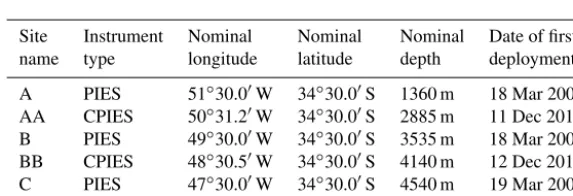
The Southwest Atlantic MOC (SAM) array was first de-ployed at 34.5◦S in March 2009 to capture the meridional flow of the western boundary currents, with the primary aim of making long-term measurements of the western boundary flows associated with the MOC (Meinen et al., 2012, 2013b). The ultimate long-term goal was also for the SAM array to be a cornerstone for the South Atlantic MOC Basin-wide Ar-ray (SAMBA) at 34.5◦S, which is coming to fruition with parallel deployments occurring on the eastern boundary in 2013 and 2014 (e.g., Ansorge et al., 2014). The SAM ar-ray involves four pressure-equipped inverted echo sounders (PIESs) deployed at depths ranging from about 1300 m down to about 4700 m, and extending roughly 650 km offshore from the outer edge of the continental shelf (see Table 1 and Fig. 1). Note that the Site B PIES (see Fig. 1) malfunctioned in 2010 and was lost during a recovery attempt in July 2011, so there is a roughly 1-year gap at that site in 2010–2011.
The array location was selected to be just north of the northern edge of the meander window of the Brazil– Malvinas Confluence (e.g., Gordon and Greengrove, 1986; Olson et al., 1988; Garzoli 1993; Goni et al., 1996, 2011;
1The term “absolute” here refers to transports which
Figure 1.Map illustrating the location of the moored instruments used in this study. Instrument types are noted in the legend; site names for the original PIES (yellow squares) are “A” through “D” from west to east; the newer CPIES (cyan diamonds) site names are “AA” and “BB”, also from west to east. Filled contours indicate bottom topography from the Smith and Sandwell (1997) data set. Color contours indicate the time-mean sea-surface temperature (◦C) from 2009–2015 from the GHRSST MUR reanalysis SST data product (see Chin et al., 1998; see also https://mur.jpl.nasa.gov/multi_resolution_analysis.php). The smaller panels on the right show the monthly mean SST maps from 2009–2015 for February (top) and August (bottom) to illustrate the latitudinal range through which the Brazil–Malvinas Confluence shifts during the year.
Table 1.Nominal locations, depths, and initial deployment dates of the PIES and CPIES moorings discussed in this paper. Note: the first instrument at Site B was a CPIES, but it was replaced with a PIES in July 2011.
Site Instrument Nominal Nominal Nominal Date of first name type longitude latitude depth deployment
A PIES 51◦30.00W 34◦30.00S 1360 m 18 Mar 2009 AA CPIES 50◦31.20W 34◦30.00S 2885 m 11 Dec 2012 B PIES 49◦30.00W 34◦30.00S 3535 m 18 Mar 2009 BB CPIES 48◦30.50W 34◦30.00S 4140 m 12 Dec 2012 C PIES 47◦30.00W 34◦30.00S 4540 m 19 Mar 2009 D PIES 44◦30.00W 34◦30.00S 4757 m 20 Mar 2009
Lumpkin and Garzoli, 2011) based on altimeter, sea-surface temperature (SST), and surface drifting buoy measurements. Depending on the precise indicator of the Brazil–Malvinas Confluence selected, the seasonal movement of the Brazil– Malvinas Confluence is characterized either by meridional shifts centered near 38.5◦S (e.g., Matano, 1993; Lumpkin and Garzoli, 2011) or by pivots around a fixed point located near 39.5◦S, 53.5◦W, changing its orientation from north–
south in austral winter to northwest–southeast in austral sum-mer (Saraceno et al., 2004). The sum-meridional extremes in the confluence location (denoted by sharp horizontal SST gradi-ents) are typically found in February and August, as can be seen in SST maps (Fig. 1, right panels).
Based on recommendations from the broad South Atlantic Meridional Overturning Circulation (SAMOC) Initiative (see www.aoml.noaa.gov/phod/SAMOC_international/), the PIES array was complemented in December 2012 with two current-and-pressure-equipped inverted echo sounders (CPIESs) as part of the parallel South Atlantic MOC Brazil
project (SAMOC-Br). These CPIES instruments were de-ployed near the midpoints of the two westernmost pairs of existing PIES moorings (Fig. 1) in order to provide better horizontal resolution across the western boundary currents.
The analysis of PIES data has become more commonplace within the scientific community over the past few decades, and their use to study the DWBC and the MOC in both the North and South Atlantic has been well documented (e.g., Meinen et al., 2006, 2012, 2013a, b). Therefore, the PIES analysis methods will only be summarized here briefly, with the remainder of the methodology details left to the refer-ences cited.
time is determined using a transducer and a high-quality crystal clock (e.g., Rossby, 1969; Watts and Rossby, 1977; Tracey and Watts, 1986). The travel-time measurements from each PIES are calibrated into daily, full-water-column pro-files of temperature, salinity, and specific volume anomaly via hydrography-derived look-up tables using the Gravest Empirical Mode (GEM) technique (e.g., Meinen and Watts, 2000). The application of the GEM method to the PIES in the SAM array was first done in Meinen et al. (2012)2; that study demonstrated that the measured travel times were accu-rate to roughly 4.4 % of the observed range when compared with concurrent CTD profile data. That study also showed that the signal-to-noise ratio (SNR) for the GEM look-up ta-bles was around 20 for depths within the main thermocline and halocline, and decreased to around 1–3 below 2000 dbar. The decreased SNR below 2000 dbar is a result of both a de-creased correspondence between the observed changes and the empirical “mode” captured by the GEM technique, and the much smaller signals themselves at these depths. Because the deep vertical shear (of density as well as horizontal ve-locity) is generally quite weak in this region, this does not represent a serious limitation for the purposes of this study.
The combined observations made by an array of PIESs are powerful, as when combined with the GEM look-up ta-bles they can provide an estimate of the absolute geostrophic velocity, i.e., the combined baroclinic (vertically sheared) plus barotropic (depth-independent) flow, as follows. Verti-cally integrating the specific volume anomaly profiles gener-ated from the GEM fields and the PIES travel-time measure-ments yields daily dynamic height anomaly profiles at each of the four instrument sites. Differences in dynamic height anomaly profiles between neighboring PIES sites provide relative geostrophic velocity profiles orthogonal to the line between the PIESs (the “baroclinic” component of the veloc-ity; e.g., Meinen et al., 2006). Differences in bottom pressure from neighboring PIES sites provide absolute geostrophic velocity variability at the bottom that can be used to reference the relative velocity profiles (the “barotropic” component of the velocity; e.g., Meinen and Watts, 2000). Due to the well-known leveling problem, the time-mean absolute geostrophic velocity at the bottom cannot be determined from the bottom pressure differences (e.g., Donohue et al., 2010). The addi-tional measurement of water velocity made by the CPIESs can characterize the flow 50 m above the seafloor. However, given that the two CPIESs were deployed much further apart than the typical velocity decorrelation length scale (e.g., Donohue et al., 2010), and given that there are only measure-ments at two locations (Fig. 1), these velocity observations
2Note: It was recently discovered that, due to a coding mistake,
the time-varying bottom-pressure derived term in the absolute ve-locity in the 2012 study was added with the incorrect sign. The full time series has been recomputed for the present study. Although the character of the absolute-transport time series changes due to this mistake, the major results of the earlier study were not impacted.
are too sparse to solve the time-mean absolute-velocity refer-ence issue. As such those velocity measurements will not be discussed further in this article, and for the purposes of this study the PIESs and CPIESs will be treated interchangeably. As time variability is the focus of this paper, the time-mean issue is not crucial for this study. However, to provide reason-able time-mean absolute-velocity profiles for discussion, the time-mean velocity from an ocean general circulation model (the model is described in the next section) at 1500 dbar was added to the velocity profiles created using the PIES data3. Note that only the time-mean velocity at only 1500 dbar is used from the model for this purpose. All time variability from the PIESs is independent of the model, as is the time-mean velocity shear profile.
Most of the detailed testing of PIES-GEM estimated ve-locities and transports has been done in the North Atlantic where independent estimates were available at concurrent lo-cations – specifically for the DWBC, this has been done at 26.5◦N (e.g., Meinen et al., 2004, 2006, 2013a). Meinen et al. (2013a) compared daily PIES-derived transports to those determined from dynamic height mooring data at 26.5◦N and showed that DWBC transports estimated from the two systems had a correlation of r=0.96, and a root-mean-square difference of 6 Sv. Furthermore, they showed that cor-relations for baroclinic transports using an assumed level of no motion at 800 dbar were similarly high. Unfortunately there are no independent absolute-transport continuous time series measurements for a similar comparison at 34.5◦S as there are at 26.5◦N. However, it can be noted that the same types of instruments are used for both arrays, and the 34.5◦S GEM SNR of∼20 in the main thermocline depth range, and of 1–3 below 2000 dbar, are similar to what is observed at 26.5◦N4.
The GEM look-up tables used herein are based on a data set of 200 CTD profiles and 365 Argo profiles collected be-fore the end of 2008. See Meinen et al. (2012) for more
de-3Note that in the earlier Meinen et al. (2012) study the model
mean velocity was added near the bottom; however, for this study the model velocity at 1500 dbar was used to avoid the signifi-cant ageostrophic velocity components in the model in the nearest-bottom grid cell. The results are not highly sensitive to this choice of reference level. Also the time-mean meridional velocities are quite similar if other numerical models are used in place of OFES, e.g., NEMO (see the description of the NEMO run used in Meinen et al., 2013b). For example, the time-mean meridional velocity for the vertical grid cell nearest 1500 dbar, averaged zonally between 51.5 and 44.5◦W, from this NEMO run (−2.4 cm s−1)is very close to the same value for the OFES run (−1.6 cm s−1).
4Note that, like all bottom pressure gauges, the PIES bottom
0 1000 2000 3000 4000 5000
Average V velocity: 2009−2014
Pressure [ dbar ] (a)
Average V velocity: OFES model
(b)
0 1000 2000 3000 4000 5000
Average V velocity: 2012−2014
Pressure [ dbar ] (c)
Average V velocity: OFES model
(d)
51°W 49°W 47°W 45°W 0 1000 2000 3000 4000 5000
Average V velocity: 2012−2014
Pressure [ dbar ] (e)
51° W 49° W 47° W 45° W
Average V velocity: OFES model
(f)
Meridional velocity [ cm s
−1 ] −40 −30 −20 −10 0 10 20
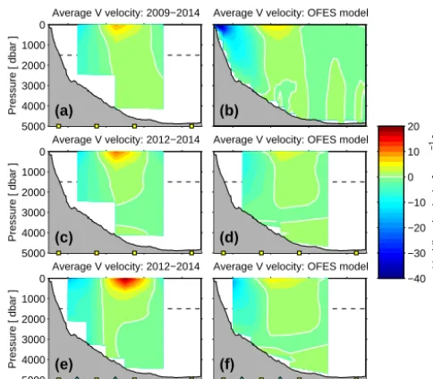
Figure 2.Time-mean meridional velocity from the PIES data (left panels) and from the OFES model (right panels). For the data-based mean sections: top panel indicates the mean over the full 5-year pe-riod for which data are available at the four PIES sites (denoted as yellow boxes on bottom axis); middle panel indicates the mean over only the∼2 years when the array was augmented, but still using only the four PIES sites; bottom panel indicates the mean over the augmented∼2 years but now using the additional CPIES sites (de-noted as cyan diamonds on bottom axis). For the model-based mean sections: top panel indicates the mean at 0.2◦horizontal grid reso-lution; middle panel indicates the time mean with the profiles hor-izontally averaged between the PIES sites; bottom panel indicates the time mean with the profiles horizontally averaged between all PIES and CPIES sites. For all panels, the gray-filled shape indicates the bottom topography from the Smith and Sandwell (1997) data set. Horizontal dashed line indicates the level where the time mean from the model is used to reference the bottom-pressure variability. White contours in all panels indicate zero flow; color contours are at 2 cm s−1intervals.
tail and an example GEM look-up table. Since the beginning of the SAM project, quasi-annual CTD sections have been collected along the PIES line, both to provide concurrent calibration for the PIES travel times and to observe finer-scale and better horizontal resolution water-mass changes over time. These CTD data have not been incorporated into the GEM fields, and as such they represent an independent data set. For this study, CTD sections from July 2010, De-cember 2010, July 2011, and DeDe-cember 2012 are averaged in a fairly simple manner solely to provide an overview of the major water masses. The CTDs collected right at the PIES sites were also used to calibrate the PIES-measured travel times into the corresponding travel times that would be ob-served on a common pressure level (e.g., Meinen and Watts, 1998).
3 Numerical model output
To aid in the interpretation of the observations from the PIES array at 34.5◦S, output from a high-quality, well-validated, numerical model was also used. The OFES (e.g., Sasaki et al., 2008) was selected for this study. The OFES model is produced by the Japan Agency for Marine-Earth Science and Technology (JAMSTEC), and it is a massively paral-lelized implementation of the National Oceanic and Atmo-spheric Administration’s Geophysical Fluid Dynamics Lab-oratory’s Modular Ocean Model version 3 (MOM3). The model equations have been discretized on a Mercator B-grid with 54 verticalzlevels and a horizontal resolution of 0.1◦.
For the analysis presented here, model fields were provided by JAMSTEC on 3-day snapshot intervals with a 0.2◦ hor-izontal grid (i.e., every other grid point) during the period 1980 through 2006. This roughly 20 km spacing is 5 to 15 times finer than the spacing between the PIES moorings in the real ocean. The OFES model was spun up for 50 years using a monthly climatology derived from National Cen-ters for Environmental Prediction–National Center for At-mospheric Research (NCEP–NCAR) reanalysis atAt-mospheric fluxes (Masumoto et al., 2004), and it then was forced with daily mean NCEP–NCAR reanalysis data from 1950 to 2006 (Sasaki et al., 2008). To avoid remaining spin-up transients, only the output from the final 27 years of the run was used for this analysis. This model run was selected because it has previously been validated against both other models and the limited available observations in the South Atlantic (Dong et al., 2011; Perez et al., 2011; van Sebille et al., 2012; Garzoli et al., 2013, 2015).
4 Results and discussion
The time-mean absolute-velocity section calculated from the PIES data during 2009–2014 via the methods de-scribed above shows the Brazil Current flowing southward between PIES sites A and B between the surface and roughly 800 dbar, with the DWBC flowing southward be-low it (Fig. 2a). These fbe-lows appear weak and smooth hor-izontally; however, keep in mind that because these veloc-ities are calculated via the geostrophic method they repre-sent a horizontal average between each pair of PIES sites – i.e., horizontal averages over 2–3◦of longitude. Also, along the SAM section west of∼49.5◦W the entire water column flows southward, so there is no obvious separation in the ve-locity section between the near-surface Brazil Current and the intermediate and deep-water flows. Immediately offshore of these southward flows, recirculations to the north in both the surface and deep layers are observed. Even further off-shore, between PIES sites C and D, the flow turns southward once again.
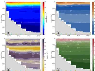
Figure 3.Average sections of in situ temperature(a), salinity(b), dissolved oxygen(c), and neutral density(d). Sections from July 2010, December 2010, July 2011, and December 2012 are averaged in a simple manner to make these plots, solely to illustrate the approximate vertical distribution of the water masses in the region.
section from the data (Fig. 2a), albeit with more finely re-solved horizontal structure. Additional horizontal informa-tion is available from the PIES/CPIES array during the final 2 years – but before looking at that structure it is instruc-tive to first evaluate the time-mean velocities derived from the original four-PIES array only during the final 2-year pe-riod (Fig. 2c). The roughly 2-year average is similar to the 4.5 year average (compare Fig. 2a and c), with the upper layer recirculation being slightly stronger and the deep ocean recirculation being slightly weaker or even slightly south-ward at some depths during the shorter 2-year average. Av-eraging the model velocity output between pairs of PIESs to simulate the geostrophic averaging (Fig. 2d) yields a section that is qualitatively similar to the 2-year average from the PIES in terms of horizontal and vertical structure, although there are some differences in intensity (compare Fig. 2c and d).
Including the two CPIES records enhances the horizon-tal structure of the time-mean section, with a more evident Brazil Current core, a stronger upper ocean recirculation core, and a deep recirculation cell that extends to the bot-tom (Fig. 2e). The model velocity output averaged between the six sites (Fig. 2f) is quite similar to the PIES/CPIES ve-locity section, although the northward recirculation in the model is weaker than observed both near the surface and at
depth. An important point to remember is that the time-mean model velocity at 1500 dbar was used to set the time-mean PIES flow at that pressure level as mentioned earlier (see dashed black lines in Fig. 2), so there is perfect agreement between the PIES/CPIES time-mean velocity and the model velocity at 1500 dbar by construction. (Apparent differences at 1500 dbar are contouring artifacts only.)
As noted earlier, at 34.5◦S, the western boundary flows in the upper and deep layers (Brazil Current and DWBC, re-spectively) overlay one another, such that the meridional ve-locities near the boundary are generally all southward from surface to bottom. One could attempt to use water-mass prop-erties to identify the level that bounds the base of the Brazil Current and the top of the DWBC; however, as will now be shown, this is not particularly satisfying or successful at this location. Average vertical sections of temperature, salinity, dissolved oxygen, and neutral density (Fig. 3) show obvi-ous water-mass layers, perhaps most clearly in the dissolved oxygen (Fig. 3c). For the purposes of the discussion of deep-water flows in this paper, the following deep-water-mass defini-tions are used following Preu et al. (2013):
51°W 49°W 47°W 45°W 0
1000
2000
3000
4000
5000
Pressure [ dbar ]
UCDW
NADW
LCDW
AABWx − northwardo − southward
Figure 4. Schematic section illustrating the observed deep wa-ter masses and their time-mean flow direction across the section. Water-mass definitions are as noted in the text, with the direction of flow denoted with either an “x” or an “o” as noted. Time mean is determined over the December 2012–October 2014 time period when all six PIES/CPIES sites are available. Water masses are deter-mined using the PIES+GEM estimated profiles. Note the dissolved oxygen criteria for UCDW cannot be tested using the PIES+GEM data, so only the neutral density criteria were employed here; evalu-ation using the CTD section data suggests that the oxygen criteria is consistently met in the depth range where the UCDW neutral den-sity criteria are satisfied.
– Upper Circumpolar Deep Water (UCDW): neutral den-sity between 27.75 and 27.90 kg m−3 with dissolved oxygen values below 4.5 mL L−1;
– North Atlantic Deep Water (NADW): neutral density between 27.90 and 28.10 kg m−3 with salinity greater than 34.8 psu;
– Lower Circumpolar Deep Water (LCDW): neutral den-sity between 28.06 and 28.20 kg m−3with salinity less
than 34.8 psu;
– Antarctic Bottom Water (AABW): potential tempera-ture less than 0◦C.
Based on these definitions, the layering of the water col-umn along the SAM array clearly shows AAIW overlay-ing UCDW, which overlays NADW, which overlays LCDW, which finally overlays the AABW. These are most evident in the oxygen section (Fig. 3c), with the enhanced oxygen values of the AAIW around 900 dbar, the NADW around 2800 dbar, and the AABW around 4800 dbar standing out from the comparatively lower oxygen waters of the UCDW and LCDW.
The time-mean locations of the main DWBC water-mass interfaces demonstrate some rather surprising results
when overlain on the time-mean meridional velocity section (Fig. 4). Very near the continental slope, the NADW is car-ried southward as one would expect in the DWBC; however, immediately offshore the entire NADW layer is being car-ried northward, essentially heading back toward the north-ern formation regions, although the array provides no infor-mation on how far to the north these waters are carried be-yond 34.5◦S. Similarly, all of the time-mean flow that can clearly be tagged as AABW at this section is headed south-ward tosouth-ward the formation region; this result appears to be robust, as small variations in the time-mean flow added at 1500 dbar from a different model (not shown) would not change these southward values (or the northward sign of the NADW mean recirculating flow). The NADW recirculation is not too surprising, as DWBC recirculations in the NADW layer have been commonly observed at many locations along the DWBC pathway through the Atlantic (e.g., Schott et al., 2005; Johns et al., 2008; Meinen et al., 2012; Hummels et al., 2015). The AABW flow to the south, on the other hand, is somewhat unexpected, as it is counter to both previous hy-drographic observations (e.g., Hogg et al., 1999; Mémery et al., 2000) and simple intuition given the location of the for-mation regions for the AABW.
absolute velocities near the boundary, and not just relative velocities.
4.1 Observed deep-flow variability
As has been noted at several other latitudes along the path-way of the DWBC, the temporal variability of the DWBC flow greatly exceeds the time-mean values (e.g., Schott et al., 2004, 2005; Toole et al., 2011; Johns et al., 2008; Send et al., 2011; Hummels et al., 2015). The deep-flow variabil-ity at 34.5◦S is no exception (Fig. 5). Most of the strongest variations in the deep flow within the NADW layer (2000– 3200 dbar; right panel in Fig. 5) are also observed in the mid-depth and surface layers (center and left panels in Fig. 5, respectively). The shear between layers is not constant; how-ever, with some events having similar transport in the NADW layer and the mid-depth layer above (see June 2009 anoma-lously northward flow event in the middle and offshore parts of the array in Fig. 5, center and right panels), while oth-ers can be much more intense in one layer than the other (see the anomalously northward flow in the May–June 2012 event and the February–March 2014 event in the offshore parts of the array in Fig. 5 where the transport signal in the NADW layer is much larger than in the mid-depth layer im-mediately above). Interestingly, these intense events in the deep layer are sufficiently large at times that the cumula-tive NADW flow integrated offshore will reverse sign (see white contours in the right panel of Fig. 5), indicating that the offshore recirculation to the north at times exceeds the southward flow of the DWBC itself. In most cases the deep flow, i.e., the flow deeper than 800 dbar, is highly correlated in terms of variability. For example, the transport integrated across the array from sites A to D within vertical limits of ei-ther 800–4800 dbar or 2000–3200 dbar yields time series that are very highly correlated5within one another (r=0.98). For the remainder of the paper, unless otherwise noted, the deep transports will be integrated between 800 and 4800 dbar (or between 800 dbar and the seafloor where shallower).
Integrating the meridional transport through the largest possible DWBC layer, from 800 down to 4800 dbar and across the entire array between sites A and D, it becomes clear that these strong events can reverse the deep flow for periods of a few days to a few months (Fig. 6, black solid line; see also Table 2 for volume transport statistics)6. The
5Some might suspect this high correlation could be artificial due
to the calculation of transport via the single “gravest” mode inher-ent in the PIES/CPIES analysis technique. While a single “mode” is used in this manner, a similar correlation analysis of the deep trans-port integrated in the OFES model yields a very similar high value (r=0.95).
6Note that the transport integrated over the full record (2009–
2014) within the 800–4800 dbar level from sites A to D does not use the data from sites AA and BB, as those two sites are only available during 2012–2014. Because of the sloping topography, the trans-ports integrated with or without sites AA and BB are slightly
dif-Table 2.Statistics for the volume transport calculated from the PIES and GEM data. The transports were integrated from sites A to D (see Table 1) and from 800 down to 4800 dbar (or the bottom, where it is shallower). Statistics were calculated over the period 2009 to 2014 using only the original PIES moorings.
Daily 30-day low-pass filter
Mean −15.2 Sv −15.2 Sv
Median −17.4 Sv −17.4 Sv
Standard Deviation 22.8 Sv 20.3 Sv Maximum value +50.1 Sv +35.0 Sv Minimum value −89.3 Sv −60.8 Sv
resulting time-mean value (−15.2 Sv) is slightly smaller than would be expected given previous moored observations up-stream at 11◦S (−16.9 Sv for the NADW layer only, Schott
et al., 2005;−17.5 Sv for the DWBC, Hummels et al., 2015). It is also slightly smaller than the averages estimated from repeated ship sections at 5◦S (e.g.,−17.3 Sv; Schott et al., 2005, estimated roughly between 800–4800 dbar from their Fig. 7a) and at 11◦S (e.g.,−22.5 Sv; Schott et al., 2005, esti-mated roughly between 800–4800 dbar from their Fig. 7b). This lower transport at 34.5◦S would be consistent with the Garzoli et al. (2015) pathway analysis that suggests that
∼20 % of the DWBC transits off toward the eastern side of the basin at around 20◦S; note that the Garzoli et al. (2015) study used the same OFES model run as one of its analysis tools, so the results are not fully independent from the re-sults presented here. The PIES mean DWBC transport value at 34.5◦S is roughly comparable with the widely varying
pre-vious estimates of the MOC upper limb at this latitude (e.g.,
−12.4 Sv from an inverse estimate using hydrographic sec-tions at 32◦S, Lumpkin and Speer, 2007;−18.1 Sv from re-peated expendable bathythermograph sections, Garzoli et al., 2013), as it should be if the bulk of the lower limb of the MOC is carried by the DWBC. However, it must be noted that due to the leveling issue discussed earlier, the time mean calculated herein for the DWBC at 34.5◦S is partially de-pendent on the OFES model velocity at 1500 dbar, as noted earlier. As such, the time mean is not the focus here.
Figure 5.Hovmoller plots illustrating the 30-day low-pass-filtered (LPF) meridional absolute transports integrated in three layers as noted in the panel titles. Transports are cumulatively integrated offshore from the shallowest site eastward toward the center of the basin. Bold white contour indicates zero meridional flow. Symbols along the bottom axes indicate the location of the PIESs and CPIESs; the upper panels show the time periods when all six sites were available.
Figure 6. Time series of DWBC volume transport determined across the full horizontal span of the array and integrated vertically from 800 to 4800 dbar (or the bottom for areas where it is shal-lower). The total absolute transport is shown (black solid), as are the components relative to an assumed level of no motion at 800 dbar (“Relative”; blue dashed) and associated with the actual reference layer flow (“Reference Layer”; red dash–dot). The gray horizontal solid and dashed lines respectively indicate the time mean and the time mean plus or minus two standard errors of the mean (i.e., the 95 % confidence limit for the mean value). Standard errors were de-termined following commonly used methods (e.g., Dewar and Bane, 1985).
day low-pass filter, the standard deviation is large (20.8 Sv) and the peak-to-peak range exceeds 95 Sv. These variations are somewhat larger than the∼80 Sv peak-to-peak range ob-served at 11◦S (e.g., Schott et al., 2005; Hummels et al., 2015); however, this likely reflects a larger integration
do-main used at 34.5◦S where the array stretches further off-shore (∼650 km versus 250 km) and captures more of the DWBC recirculation. As will be shown shortly, integrating the transport at 34.5◦S to a roughly similar 200 km distance offshore (i.e., the total longitudinal extent of the 11◦S west-ern array) yields smaller peak-to-peak transport of∼60 Sv, which is more comparable with the previous values observed at 11◦S.
J F M A M J J A S O N D J −60
−40 −20 0 20 40 60
Transport anomaly [ Sv ]
Figure 7. Annual cycle of DWBC volume transport (integrated 800–4800 dbar across the entire array); transport anomalies are shown relative to the record-length mean. Gray lines are individual years; red line is the average of all years. Transport time series was low-pass filtered with a 30-day cutoff period to reduce the higher frequency signals.
is highly correlated with the reference transport (r=0.91), and is not significantly correlated with the relative transport (r=0.14); however, that is not to say that the relative con-tribution is unimportant. While the relative term is typically 10 Sv or less, in some events it greatly exceeds this value, with one event in late 2009 having a southward relative trans-port exceeding 40 Sv in amplitude for more than a month. In addition to illustrating the fact that the “baroclinic” term and the “barotropic” term are uncorrelated, consistent with what has been observed at this location with the first year of data along 34.5◦S (Meinen et al., 2012) and at other latitudes (e.g., 26.5◦N; Meinen et al., 2013a), these results make clear
that both the “baroclinic” and the “barotropic” terms must be measured directly to quantify the DWBC flow.
4.2 Spectral distribution of observed DWBC energy
When the first year of data at 34.5◦S was published (Meinen et al., 2012), it was not possible to evaluate whether there was an annual cycle in the DWBC transport, although anal-ysis of the OFES model at that time suggested that there was a very weak, albeit not significant, seasonal signal. With nearly 5 years of real data now available, this can be revisited (Fig. 7). With the additional years there is still no obvious an-nual cycle in the data, even after applying a 30-day low-pass filter to eliminate the higher-frequency signals. The average annual cycle (red line in Fig. 7) perhaps hints at a northward anomaly in the first half of the year and a southward anomaly in the second half of the year, consistent with the earlier anal-ysis of the OFES model (Meinen et al., 2012). This observed annual signal is very weak and is highly influenced by other timescales and aliasing. Interestingly, at 26.5◦N the pattern is initially the same, as there is no meaningful annual cycle
in the DWBC integrated out to∼500 km from the bound-ary (Meinen et al., 2013a). At 26.5◦N, if the DWBC is
in-tegrated over a narrower domain spanning only the “mean” location of the DWBC and not including the recirculations offshore, then an annual cycle is apparent. Following the same idea here for 34.5◦S, the annual cycle was explored for the deep transport integrated only between sites A and B, which spans the “mean” location of the DWBC at this lat-itude (see Fig. 2). Unlike at 26.5◦N, there is still no clear annual cycle at 34.5◦S even when integrated across this nar-rower span, and the amplitudes are a factor of 2–4 smaller (not shown). Whether this is a dynamical difference between the two latitudes or merely a sign that additional years of data are needed to tease out the annual cycle at 34.5◦S is an area for future research. However, it should be noted that the con-tinuous DWBC record integrated similarly at 11◦S shows no obvious stable annual cycle either (e.g., Dengler et al., 2004; Schott et al., 2005).
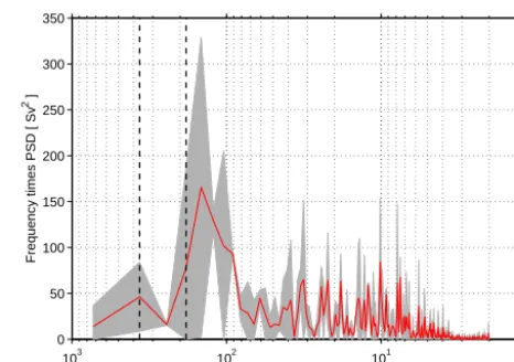
Spectral analysis of the continuous portion (2011–2014) of the absolute-transport time series (integrated from sites A to D) finds little energy at either the semi-annual or annual periods, with the largest signature being a broad peak span-ning periods of 90–160 days centered near 145 days (Fig. 8; spectra are plotted in variance-preserving form, so the area under the curve is proportional to the energy at each period). The relatively short record compared to this timescale results in fairly wide error bars for the spectrum, so the spectral dis-tribution may yield more nuanced results once a few more years of data have been collected. There are noisy spectral peaks in the 20–50 day band. Previous observations focusing on the upper ocean just south of the SAM array (near 37 to 38◦S) by Garzoli and Simionato (1990) found wave signals
Table 3.Distribution of variance in the indicated period bands in the DWBC transport calculated from the PIES/CPIES observations during the continuous 2011–2014 window. The observed DWBC transport was integrated between 800 and 4800 dbar and between the original PIES at sites A and D. Values for transport integrated only between the PIES at sites A and B are shown in parentheses.
Period band (days) Variance Percentage of [Sv2] total variance
2 to 50 103.3 (83.1) 28.4 (25.9) 50 to 170 153.4 (61.0) 42.1 (19.0) 170 to 190 7.7 (54.9) 2.1 (17.1) 190 to 350 39.3 (54.0) 10.8 (16.8) 350 to 390 7.5 (54.9) 2.1 (17.1) 390 to record length 53.0 (12.8) 14.5 (4.0)
when integrated within that zonal span, despite there being no obvious visual annual cycle.
4.3 Characterizing the deep-flow variations
Characterizing the nature of these flow variations could be approached via Empirical Orthogonal Function analysis (e.g., Emery and Thomson, 1997); however, the resulting eigenvalues are not statistically significant from one another – i.e., they are “degenerate” (North et al., 1982) and cannot be physically interpreted in a meaningful way, which may be at least partially due to the relatively short record length. Instead, to characterize the vertical-horizontal structure of these transport variations, composite averages were created based on the transport integrated from 800 to 4800 dbar (or the bottom where shallower) and from sites A to D (i.e., the black line in Fig. 6). Composite mean sections of meridional velocity were created for “strong” days, where the southward transport, integrated within the above-described bounds, was greater than the record-length time mean plus two statisti-cal standard errors of the mean (the standard error was esti-mated to be 5.2 Sv based on the estiesti-mated integral timescale of 17 days; see solid and dashed gray lines in Fig. 6), for “weak days” where the southward transport was less than the record-length time mean minus two statistical standard errors of the mean, and for “middle” days with transports within±two statistical standard errors around the time mean (Fig. 9). Only the time period where the additional instru-ments at sites AA and BB were available was used in creating the composites as this provides the best horizontal resolution of data.
The resulting composites suggest that the anomalous flows have a certain “barotropicity” inshore of around 49◦W, with stronger southward DWBC flows below 1000 dbar corre-sponding to stronger southward Brazil Current flows above 1000 dbar on “strong” days, and weaker southward flow in shallow and deep layers on “weak” days (Fig. 9). There is also a hint of an offshore shift of the deep flow on weak
100 101
102 103
0 50 100 150 200 250 300 350
Frequency times PSD [ Sv
2 ]
Period [ days ]
Figure 8. Variance-preserving spectrum of the DWBC volume transport using the continuous record that begins in July 2011. Spec-trum determined using Welch’s averaged periodogram method and a 2-year window allowing 1 year of overlap. Gray shading indicates the 95 % confidence limits. Vertical black dashed lines indicate the annual and semi-annual periods.
days. The zero crossing locations (white contours in Fig. 9) seem to be fairly constant in the upper layer, while below roughly 2000 dbar this is not true. By contrast to the appar-ent barotropicity of the flows near to the continappar-ental slope, offshore of around 49◦W the composite results suggest sig-nificant “baroclinicity” (i.e., increased vertical shear), with weak northward flow (or even southward flow) at depth but intensified northward flow near the surface on “strong” days, but reduced baroclinicity (i.e., reduced shear) on the “weak” days. Recall that the definition for “strong” and “weak” here is based on the integral of the deep flow across the entire sec-tion, so in phase flow anomalies in the deep layer are perhaps an artifact of how the composites are created. Correlation of the deep flows between pairs of PIES/CPIES is quite low, so blending the inshore and offshore deep flows may not pro-vide the clearest separation of events, although integrating the deep flow across the array should in theory provide the best estimate of the “throughput” of the DWBC by attempt-ing to average out the recirculation offshore. As has been noted in the North Atlantic at 26.5◦N however, these recir-culations may reach all the way to the Mid-Atlantic Ridge (Meinen et al., 2013a), which if also true at 34.5◦S would suggest that some of the recirculation is beyond the range of the array (note that at 34.5◦S the Mid-Atlantic Ridge is about
2500 km east of site D).
Figure 9.Composite meridional velocity sections based on the average of all data when the enhanced array is in place, December 2012– October 2014 (top left), the average of all days when the southward DWBC transport is within±2 standard errors around the mean value (“middle” – lower left), the average of the days where the southward DWBC transport is weaker than the mean minus 2 standard errors (“weak” – top right), and the average of the days where the southward DWBC transport is stronger than the mean plus 2 standard errors (“strong” – lower right). Gray shading indicates bottom topography; symbols along the bottom of each panel indicate the PIES and CPIES sites. Note the color-bar range is different than for Fig. 2. White contours in all panels indicate zero flow.
Jan 13 Apr 13 Jul 13 Oct 13 Jan 14 Apr 14 Jul 14 Oct 14 −50
−40 −30 −20 −10 0 10
Transport [ Sv ]
Figure 10. Time series of absolute transport integrated between sites A and B, and between 800 and 4800 dbar (or the bottom), dur-ing the period when all instruments were in place. Also shown is the time-mean value (gray solid line) and lines corresponding to the time mean plus or minus 2 standard errors of the mean (gray dashed), i.e., the 95 % confidence limit for the mean value. Standard errors were determined following commonly used methods (e.g., Dewar and Bane, 1985).
than half that of the deep transport integrated across the entire array (Table 4), but the peak-to-peak range still exceeds 50 Sv within the narrower span. The statistical standard error of the mean is 1.1 Sv, and the integral timescale is about 6 days, suggesting that higher frequencies play a larger role in the observed variability in the narrower span between sites A and
B. The “strong” and “weak” days in the record were again defined as days where the meridional transport experienced southward or northward anomalies greater than two statis-tical standard errors, respectively. The resulting composites (Fig. 11) show similarities to the earlier versions (Fig. 9) inshore of about 49◦W, with the anomalous flow having significant barotropicity. The near-slope anomalies are even stronger in these composites, with noticeably stronger flows at all depths on the “strong” days (compare the lower right panels of Figs. 9 and 11), and much weaker flows at all depths on the “weak” days (compare the top right panels of Figs. 9 and 11). Offshore of 49◦W, the composites are
re-circulations are associated with strong Brazil Current events (Fig. 11d).
This apparent anti-correlation between the deep flow near the slope and the recirculation offshore is somewhat surpris-ing, since as was noted earlier, there is only a very weak correlation between the flow between pairs of PIESs. The correlation values between the deep flows integrated in the sites A to B span and the deep flows integrated in the sites B to C span is about r=-0.4. Based on the average integral timescale for these two records (8 days) and the record length, this correlation value is statistically significantly dif-ferent from zero at even the 99 % level (cutoffr= |0.38|), but a linear relationship between the two would explain less than 20 % of the observed variability. Lagged correlations show insignificant values with a shift of more than a few days in either direction, and this is true for not only the daily records but also for records that have been low-pass filtered (2nd order Butterworth passed both forward and back) with cut-off periods of 10, 30, and 90 days. So while the composites suggest that on average the offshore recirculation intensifies when the southward DWBC flow increases, and vice versa, the actual flow at any given time is more complex and nu-anced (e.g., may have shorter spatial scales with banded flow structures). Clearly the deep flow in this region is influenced by many different factors, but the observational array, while well suited to capturing the deep meridional transport vari-ability near the western boundary, has limited vari-ability to track deep-flow features migrating into the region. Therefore, an evaluation in a numerical model may aid in the interpretation of the observed signals and help extract more information (as was also done in the earlier Meinen et al., 2012 study).
4.4 Modeled deep-flow variability
Integrating the meridional velocity from the OFES model within the same longitudinal range (between sites A and D) and over the same pressure range (800 to 4800 dbar or the bottom where it is shallower), using the 27 years of model output, yields a robust DWBC with a time mean similar to the observed value (Fig. 12, see also Table 5). While the time-mean values are similar (recall that the model 1500 dbar mean value is imposed on the data, and therefore the means are not completely independent), the time variability from the model is somewhat smaller than that of the real ocean (standard deviation of 16.5 Sv versus 22.8 Sv, respectively). As in the real ocean, there is little sign of an annual cycle in the model DWBC transport – perhaps a hint of anomalous northward flow in the first half of the year (Fig. 12, lower panel), and anomalous southward flow in the second half, but the variability at other timescales clearly dominates. The per-centage of variance explained by the annual or semi-annual periods is less than 10 % each (Table 6), although the annual and semi-annual percentage values are a factor of 2–3 larger than the comparable values for the observed time series (Ta-ble 3). Because the model output record is much longer than
the real data set, it is possible to evaluate how much energy is in the longer periods; evaluation both in period bands (Ta-ble 6) and as a spectrum (Fig. 13) illustrates that the DWBC in the model does not have much energy at periods longer than 2 years. Even using extended windows for calculat-ing the spectra does not extract much energy at the longer timescales (compare Fig. 13b, c, and d). What is clear is that the model variability is weaker than that in the actual ob-servations at essentially all timescales (compare Fig. 13a to b–d). Nevertheless, the model does show a broad peak of en-ergy centered around 140–160 days, just as the observations show, so it is clear that in general the model DWBC has sim-ilar, if perhaps too weak, variability when compared to that of the real ocean.
Having verified that the DWBC variability in the model is qualitatively similar to that in the real ocean (for periods shorter than 2 years), it is reasonable to then “step back” and evaluate a larger domain within the model to try and iden-tify the sources and/or mechanisms behind the variations ob-served near the continental slope. As a first step toward this goal, a Hovmoller plot of the OFES meridional velocity at the central depth of the NADW near 2600 m across 34.5◦S between the western continental slope and the Mid-Atlantic Ridge illustrates the presence of waves and/or eddies prop-agating both eastward and westward to the west of 40◦W (Fig. 14). The eastward-trending features have propagation speeds of roughly 5–8 cm s−1(4.5–7.0 km day−1), while the westward-trending features west of 40◦W have propagation speeds of roughly 3–4 cm s−1 (2.5–3.5 km day−1). East of about 40◦W, the flow in the model is dominated by relatively weak features that propagate westward at a much slower speed – roughly 1 cm s−1(0.9 km day−1). These weaker
fea-tures do not seem to propagate to the western portion of the basin, although it may be that they are simply obscured by the more energetic, faster features found within approx-imately 1000 km of the shore. The propagation speeds for the region west of 40◦W are in rough agreement with those found in an earlier inverted echo sounder (IES) array lo-cated just south of the PIES/CPIES array discussed herein (Garzoli and Simionato, 1990). This earlier study found that the eastward-propagating signals had the characteristics of TRWs, and given the similar or perhaps even slightly steeper topography in the study region discussed in this study, such a diagnosis seems equally likely here.
Figure 11.Same as Fig. 9, except that the transport time series used for identifying strong and weak southward transport days was integrated only between sites A and B (i.e., the record in Fig. 10) instead of between sites A and D. White contours in all panels indicate zero flow.
Table 4.Statistics for the volume transport calculated from the PIES and GEM data across the whole array (columns 2 and 3) versus only within the span between sites A and B (columns 4 and 5). Note that column 2 is identical to column 2 in Table 2. The transports were integrated from between the indicated sites (see Table 1) and from 800 down to 4800 dbar (or the bottom where it is shallower). Statistics are shown for both the period 2009 to 2014 (columns 2 and 4) and during the enhanced array period 2012–2014 (columns 3 and 5). The transports were calculated using only the original PIES moorings; the results in the enhanced period are very similar if the CPIESs are also included, as is to be expected for geostrophic calculations.
Integration span Sites A to D Sites A to B
Integration period 2009–2014 2012–2014 2009–2014 2012–2014
Mean −15.2 Sv −18.0 Sv −17.4 Sv −17.2 Sv
Median −17.4 Sv −19.8 Sv −17.2 Sv −16.9 Sv
Standard Deviation 22.8 Sv 23.0 Sv 8.1 Sv 8.3 Sv Maximum value +50.1 Sv +50.1 Sv +18.1 Sv +4.7 Sv Minimum value −89.3 Sv −68.9 Sv −46.5 Sv −46.5 Sv
Table 5.Time mean and temporal standard deviation (SD) of the volume transport integrated between 800 and 4800 dbar (or the bot-tom where shallower) and between the indicated PIES locations. The observation-based estimates (middle columns) were calculated over the 2009–2014 time period; the model-based estimates (right two columns) were calculated over the 27-year run described in the text.
Integration Data Data Model Model
span mean SD mean SD
Sites A to B −17.4 Sv 8.1 Sv −17.6 Sv 7.6 Sv Sites A to D −15.2 Sv 22.8 Sv −16.0 Sv 16.5 Sv
Waves, since they are closed circulation features that can translate properties, which waves cannot do (e.g., Chelton et al., 2007). More recently, Polito and Sato (2015) have shown that the dynamics may in fact be slightly more nuanced, pre-senting evidence that these eddies tend to “ride” on Rossby Waves.
1980 1982 1984 1986 1988 1990 1992 1994 1996 1998 2000 2002 2004 2006 −120
−100 −80 −60 −40 −20 0 20 40 60
OFES model transport [ Sv ]
Integrated from site A to site D and from 800 to 4800 dbar (or the bottom)
Absolute Relative Reference layer
J F M A M J J A S O N D J
−60 −40 −20 0 20 40 60
Transport anomaly [ Sv ]
(a)
(b)
Figure 12.Time series of DWBC volume transport calculated from output of the OFES numerical model run described within the text. Transport was integrated within 800 to 4800 dbar and between the longitudes of the real-world PIES at sites A and D. Top panel: the complete time series of absolute transport, with the every-3-day full resolution, is shown as the black solid line, while the relative and reference contributions calculated as in Fig. 6 are shown in blue dashed and red dash–dot lines, respectively. Bottom panel: annual cycle of the model DWBC transport anomaly, calculated and shown in the same manner as for the observational record shown in Fig. 7.
Table 6.Distribution of variance in the indicated period bands in the DWBC transport calculated from the OFES model output. The model DWBC transport was integrated between 800 and 4800 dbar and between the longitudes of the real locations for the PIESs at sites A and D.
Period band (days) Variance Percentage of [Sv2] total variance
6 to 50 60.0 19.2
50 to 170 105.7 33.8
170 to 190 20.8 6.7
190 to 350 56.9 18.2
350 to 390 27.3 8.7
390 to 1000 28.1 9.0
1000 to record length 13.6 4.3
NADW component of the DWBC) during the last 5 months of 1987 and comparing them to the long-term mean velocity easily highlights a closed circulation feature that causes this westward-propagating southward velocity anomaly (Fig. 15). The long-term mean from the model (Fig. 15a) clearly shows the southward DWBC hugging the continental slope at the latitude of the PIES/CPIES array (yellow line), while in the long-term mean field there is only quite weak circu-lation in comparison in the offshore portions of the array. The monthly averages from the model for the final 5 months
of 1987 (Fig. 15b–f); however, illustrate the highly ener-getic flows that can be found offshore at any particular time. A strong anticyclonic feature, highlighted by the magenta disc in Fig. 15, slowly propagates westward from August through December 1987. The radius of the disc of anticy-clonic flow, which was subjectively determined based on the mapped velocities, is roughly 180–200 km for most of the months shown (except for December, Fig. 15f, when it drops to around 120 km). The baroclinic Rossby Radius (NH/f, where the Brunt–Väisälä frequencyN=0.0018 s−1is a typ-ical mid-depth value, the water depth H=4500 m, and f
is the Coriolis parameter) in this area is roughly 100 km in the real world, so about a factor of two smaller than the ob-served anticyclonic feature. (N.B. – the barotropic Rossby Radius, given by (gH )1/2/f, where g is gravity, is much larger, around 2500 km at this latitude.) As such, referring to these propagating features as “coherent vortices” is per-haps more appropriate, but some of the features may repre-sent long Rossby Waves (Polito and Sato, 2015). Regardless, it is clear that these large westward-propagating features are creating the largest transport anomalies in the deep layers in the model, and the correspondence between model and ob-servations where it can be tested suggests that this is likely true in the real ocean as well.
5 Conclusions
As has been found at other locations along the DWBC path through the Atlantic, at 34.5◦S the time-varying intensity of the DWBC volume transport during 2009–2014 (22.8 Sv standard deviation, and peak-to-peak range of 139.4 Sv) greatly exceeds the time-mean value (−15.2 Sv) – which il-lustrates the necessity of continuous observation to avoid aliasing. The spectral character of the observed variability has a broad peak within roughly 90–160 days, centered near 145 days, with additional energy found in the 20–50 day band. Composite analysis (integrated between both sites A to D and sites A to B) suggests that the variations near the continental slope west of 49◦W have some barotropicity, in the sense that they affect the flow at all layers including those near the sea surface. The composite results also show that the strong southward transport anomalies near the slope are partially compensated by increased recirculation to the north immediately offshore of 49◦W, while weak southward trans-port anomalies near the slope are also partially compensated by decreased recirculation to the north offshore of 49◦W.
0 50 100 150 200
Frequency times PSD [ Sv
2 ] (a) (b)
100
101
102
103
104
0 50 100 150 200
Frequency times PSD [ Sv
2 ]
Period [ days ]
(c)
100
101
102 103
104
Period [ days ]
(d)
Figure 13.Variance-preserving spectra of the DWBC volume transport time series (integrated from 800 to 4800 dbar and between PIES sites A and D).(a)Spectrum for the observational record – as in Fig. 8 but restricting theyaxis range for comparison purposes.(b)Spectrum for the DWBC transport calculated from the OFES numerical model output within the same pressure and longitude bounds and utilizing a 2-year window length with 50 % window overlap.(c)Same as panel b but using a 9-year window length with 50 % window overlap.(d)Same as(b)but using an 18-year window length with 50 % window overlap. For all panels the gray shaded region represents the 95 % confidence limits for the calculated spectrum. All spectra determined using the Welch’s averaged periodogram method.
Figure 15.Velocities from the OFES model at the core of the NADW near 2600 m depth:(a)average over the full 27-year run described in the text;(b)average over August 1987;(c)average over September 1987;(d)average over October 1987;(e)average over November 1987; and(f)average over December 1987. Land is denoted by green; bottom topography is from the Smith and Sandwell (1997) data set. Yellow line denotes nominal location of the PIES/CPIES array in the real ocean. Magenta disc highlights the propagating eddy and/or wave feature discussed in the text.
vortices. This suggests that the observing array might be enhanced or improved through the addition of either or both increased horizontal resolution of observations (to more clearly identify these propagating features) and/or the ex-pansion of the array out toward the Mid-Atlantic Ridge (to more completely capture the offshore recirculations). The results also demonstrate the necessity of directly and independently capturing both the “baroclinic” (vertically sheared) and “barotropic” (vertically constant) flows in or-der to properly unor-derstand the absolute-transport variability of the DWBC at this location.
Data availability. The moored data used in this study are available at http://www.aoml.noaa.gov/phod/research/moc/samoc/sam/data_ access.php and/or via email communication with the lead author.
Competing interests. The authors declare that they have no conflict of interest.
Acknowledgements. The authors would like to thank the ship captains and crews of the NH Cruzeiro do Sul, ARA Puerto Deseado, SVIce Lady Patagonia II, N.Oc.Alpha-Crucis, and the N.Oc. Alpha Delphini, who have all ably supported our research cruises and project. Ulises Rivero, Rigoberto Garcia, Pedro Peña, Carlos Franca, Marcela Charo, Daniel Valla, and the support teams in Miami, São Paulo and Buenos Aires have all helped collect and process the data presented herein. The US PIES/CPIES
observations and the participation of Christopher S. Meinen, Sil-via L. Garzoli, Renellys C. Perez, and Shenfu Dong were supported via the NOAA Climate Program Office’s Climate Observations Division (FundRef number 100007298) under the Southwest Atlantic Meridional Overturning Circulation (SAM) project, with additional support from the NOAA Atlantic Oceanographic and Meteorological Laboratory. Silvia L. Garzoli and Renellys C. Perez were also supported in part under the auspices of the Cooperative Institute for Marine and Atmospheric Studies (CIMAS), a Cooper-ative Institute of the University of Miami and NOAA, cooperCooper-ative agreement NA10OAR4320143. RP acknowledges additional support from NOAA (grant NA13OAR4310131) and NASA (grant NNX14AH60G). The Brazilian CPIES observations were supported by the São Paulo State Research Foundation (FAPESP) through the SAMOC-Br project (grant 2011/50552-4). EC ac-knowledges CNPq for a Research Fellowship (grant 302018/2014-0). Hydrographic observations were partially supported by the Inter-American Institute for Global Change Research (IAI) grants SGP2076 and CRN3070. The IAI is supported by the US National Science Foundation (grants GEO-0452325 and GEO-1128040). The merged, multi-sensor L4 Foundation sea-surface temperature (SST) data used herein were provided by the NASA Jet Propulsion Laboratory under support from the NASA MEaSUREs program. Rick Lumpkin and Arthur Mariano provided several helpful ideas while the manuscript was being prepared, and Libby Johns, Shane Elipot, and two anonymous reviewers gave a number of suggestions for improving earlier drafts of the paper.
Edited by: M. Hecht
References
Ansorge I., Baringer, M., Campos, E., Dong, S., Fine, R. A., Gar-zoli, S., Goni, G., Meinen, C., Perez, R., Piola, A., Roberts, M., Speich, S., Sprintall, J., Terre, T., and van den Berg, M.: Basin-Wide Oceanographic Array Bridges the South Atlantic, EOS Transactions, AGU, 95, 53–54, doi:10.1002/2014EO060001, 2014.
Arhan, M., Mercier, H., and Park, Y.-H.: On the deep water circu-lation of the eastern South Atlantic Ocean, Deep-Sea Res. Pt. I, 50, 889–916, doi:10.1016/S0967-0637(03)00072-4, 2003. Bryden, H. L., King, B. A., and McCarthy, G. D.: South
At-lantic overturning circulation at 24◦S, J. Mar. Res., 69, 39–56, doi:10.1357/002224011798147633, 2011.
Buckley, M. W. and Marshall, J.: Observations, inferences, and mechanisms of the Atlantic Meridional Overturn-ing Circulation: A review, Rev. Geophys., 54, 5–63, doi:10.1002/2015RG000493, 2016.
Chelton, D. B. and Schlax, M. G.: Global observations of oceanic Rossby Waves, Science, 271, 234–238, 1996.
Chelton, D. B., Schlax, M. G., Samelson, R. M., and de Szoeke, R. A.: Global observations of large oceanic eddies, Geophys. Res. Lett., 34, L15606, doi:10.1029/2007GL030812, 2007.
Chin, T. M., Milliff, R. F., and Large, W. G.: Basin-Scale, High-Wavenumber Sea Surface Wind Fields from a Multiresolution Analysis of Scatterometer Data, J. Atmos. Ocean. Tech., 15, 741–763, 1998.
Coles, V. J., McCartney, M. S., Olson, D. B., and Smethie Jr., W. M.: Changes in Antarctic Bottom Water properties in the western South Atlantic in the late 1980s, J. Geophys. Res., 101, 8957– 8970, 1996.
De Leon, Y. and Paldor, N.: Linear waves in midlatitudes on the rotating spherical Earth, J. Phys. Oceanogr., 39, 3204–3215, doi:10.1175/2009JPO4083.1, 2009.
Dengler, M., Schott, F. A., Eden, C., Brandt, P., Fischer, J., and Zantopp, R.: Break-up of the Atlantic Deep Western Bound-ary Current into eddies at 8◦S, Nature, 432, 1018–1020, doi:10.1038/nature03134, 2004.
Dewar, W. K. and Bane, J. M.: Subsurface Energetics of the Gulf Stream near the Charleston Bump, J. Phys. Oceanogr., 15, 1771– 1789, 1985.
Dijkstra, H. A.: Characterization of the multiple equilibria regime in a global ocean model, Tellus A, 59, 695–705, 2007.
Dong, S., Garzoli, S. L., Baringer, M. O., Meinen, C. S., and Goni, G. J.: The Atlantic Meridional Overturning Circulation and its Northward Heat Transport in the South Atlantic, Geophys. Res. Lett., 36, L20606, doi:10.1029/2009GL039356, 2009.
Dong, S., Garzoli, S. L., and Baringer, M. O.: The role of inter-ocean exchanges on decadal variations of the northward heat transport in the South Atlantic, J. Phys. Oceanogr., 41, 1498– 1511, 2011.
Dong, S., Baringer, M. O., Goni, G. J., Meinen, C. S., and Garzoli, S. L.: Seasonal variations in the South At-lantic Meridional Overturning Circulation from observations and numerical models, Geophys. Res. Lett., 41, 4611–4618, doi:10.1002/2014GL060428, 2014.
Dong, S., Goni, G., and Bringas, F.: Temporal variability of the Meridional Overturning Circulation in the South Atlantic be-tween 20◦S and 35◦S, Geophys. Res. Lett., 42, 7655–7662, doi:10.1002/2015GL065603, 2015.
Donohue, K. D., Watts, D. R., Tracey, K. L., Greene, A. D., and Kennelly, M.: Mapping circulation in the Kuroshio Ex-tension with an array of current and pressure recording in-verted echo sounders, J. Atmos. Ocean. Tech., 27, 507–527, doi:10.1175/2009JTECHO686.1, 2010.
Drijfhout, S. S., Weber, S. L., and van der Swaluw, E.: The stabil-ity of the MOC as diagnosed from model projections for pre-industrial, present and future climates, Clim. Dynam., 37, 1575– 1586, doi:10.1007/s00382-010-0930-z, 2011.
Emery, W. J. and Thomson, R. E.: Data Analysis Methods in Phys-ical Oceanography, Pergamon, Oxford, UK, 1997.
Frajka-Williams, E., Cunningham, S. A., Bryden, H. L., and King, B. A.: Variability of Antarctic Bottom Water at 24.5◦N in the Atlantic, J. Geophys. Res., 116, C11026, doi:10.1029/2011JC007168, 2011.
Frajka-Williams, E., Meinen, C. S., Johns, W. E., Smeed, D. A., Duchez, A., Lawrence, A. J., Cuthbertson, D. A., McCarthy, G. D., Bryden, H. L., Baringer, M. O., Moat, B. I., and Rayner, D.: Compensation between meridional flow components of the At-lantic MOC at 26◦N, Ocean Sci., 12, 481–493, doi:10.5194/os-12-481-2016, 2016.
Ganachaud, A. and Wunsch, C.: Large-Scale Ocean Heat and Fresh-water Transports during the World Ocean Circulation Experi-ment, J. Climate, 16, 696–705, 2003.
Garzoli, S. and Simionato, C.: Baroclinic instabilities and forced oscillations in the Brazil/Malvinas confluence front, Deep-Sea Res., 37 1053–1074, 1990.
Garzoli, S. L.: Geostrophic velocity and transport variability in the Brazil-Malvinas Confluence, Deep-Sea Res. Pt. I, 40, 1379– 1403, 1993.
Garzoli, S. L. and Baringer, M. O.: Meridional heat transport de-termined with expendable bathythermographs, Part II: South At-lantic transport, Deep-Sea Res. Pt. I, 54, 1402–1420, 2007. Garzoli, S. L. and Matano, R.: The South Atlantic and the Atlantic
Meridional Overturning Circulation, Deep-Sea Res. Pt. II, 58, 1837–1847, doi:10.1016/j.dsr2.2010.10.063, 2011.
Garzoli, S., Baringer, M. O., Dong, S., Perez, R., and Yao, Q.: South Atlantic meridional fluxes, Deep-Sea Res. Pt. I, 71, 21– 32, doi:10.1016/j.dsr.2012.09.003, 2013.
Garzoli, S. L., Dong, S., Fine, R., Meinen, C., Perez, R. C., Schmid, C., van Sebille, E., and Yao, Q.: The fate of the Deep Western Boundary Current in the South Atlantic, Deep-Sea Res. Pt. I, 103, 125–136, doi:10.1016/j.dsr.2015.05.008, 2015.
Goni, G., Kamholz, S., Garzoli, S., and Olson, D.: Dynamics of the Brazil-Malvinas Confluence based on inverted echo sounders and altimetry, J. Geophys. Res., 101, 16273–16289, 1996. Goni, G. J., Bringas, F., and DiNezio, P. N.: Observed low frequency
variability of the Brazil Current front, J. Geophys. Res., 116, C10037, doi:10.1029/2011JC007198, 2011.
Gordon, A. L. and Greengrove, C. L.: Geostrophic circulation of the Brazil-Falkland confluence, Deep-Sea Res., 33, 573–585, 1986. Hogg, N. G. and Owens, W. B.: Direct measurement of the deep
cir-culation within the Brazil Basin, Deep-Sea Res. Pt. II, 46, 335– 353, 1999.