A New Extremely Flexible Version of the Exponentiated Weibull Model: Theorem and Applications to Reliability and Medical Data Sets

A New Extremely Flexible Version of The Exponentiated Weibull

Model: Theorem and Applications to Reliability and Medical Data Sets

Mohamed Aboraya

Department of Applied Statistics and Insurance, Damietta University, Egypt.

[email protected]

Abstract

In this work, a new lifetime model is introduced and studied. The major justification for the practicality of the new model is based on the wider use of the exponentiated Weibull and Weibull models. We are also motivated to introduce the new lifetime model since it exhibits decreasing, upside down-increasing, constant, increasing-constant and J shaped hazard rates also the density of the new distribution exhibits various important shapes. The new model can be viewed as a mixture of the exponentiated Weibull distribution. It can also be considered as a suitable model for fitting the symmetric, left skewed, right skewed and unimodal data. The importance and flexibility of the new model is illustrated by four read data applications.

Keywords: Burr-Hatke Differential Equation; Exponentiated Weibull; Maximum Likelihood Estimation; Generating Function; Moments.

1. Genesis of the new model

A random variable (R.V.) 𝑇 is said to have the Exponentiated Weibull (EW) distribution (see Mudholkar and Srivastava (1993), Mudholkar et al., (2015) and Nadarajah et al., (2013)) if its probability density function (P.D.F.), cumulative distribution function (C.D.F.) and the reliability function (R.F.) are given by

𝑔𝐸𝑊(𝑡 ; 𝛼 , 𝛽) = 𝛼𝛽𝑡𝛽−1[1 − 𝑒𝑥𝑝(−𝑡𝛽)]𝛼−1𝑒𝑥𝑝(−𝑡𝛽),

𝐺_𝐸𝑊(𝑡 ; 𝛼 , 𝛽) = [1 − 𝑒𝑥𝑝(−𝑡𝛽_)]𝛼_, and

𝑅𝐸𝑊(𝑡) = 𝐺𝐸𝑊(𝑡 ; 𝛼 , 𝛽) = 1 − 𝐺𝐸𝑊(𝑡 ; 𝛼 , 𝛽) = {1 − [1 − 𝑒𝑥𝑝(−𝑡𝛽)]𝛼},

respectively, for 𝑡 > 0 , 𝛼 > 0 and 𝛽 > 0 . When 𝛼 = 1 we get the standard one parameter W model (see Weibull (1951)). In statistical literature, the Burr-Hatke differential equation (B.H.D.E.) can be written as

𝑑𝐹/𝑑𝑡 = 𝑔(𝑡, 𝐹)𝐹(1 − 𝐹) with 𝐹₀ = 𝐹(𝑡₀)|_{[𝑡0∈ℜ]}, (1)

where 𝐹(𝑡) = 𝐹 is the C.D.F. of a continuous R.V. 𝑇 and 𝑔(𝑡, 𝐹) is an arbitrary positive function (𝑔(+)) for any 𝑡0 ∈ ℜ . Using (1), Maniu and Voda (2008) introduced and studied the BH distribution with C.D.F. and P.D.F. given by

𝐹(𝑡 ; 𝜃) = 1 −(𝑡 + 1)−1

𝑒𝑥𝑝(𝑡𝜃) |[𝑡>0,𝜃>0],

and

𝑓(𝑡 ; 𝜃) =(𝑡 + 1)−2[𝜃(𝑡 + 1) + 1]

respectively. By replacing 𝑡 by {− 𝑙𝑜𝑔[𝐺𝐸𝑊(𝑥)]}, Yousof et al., (2018) introduced a new flexible family of distributions called the BH-G family of distributions. Based on Yousof et al., (2018), the C.D.F. of the BHEW distribution can be defined as

𝐹_{𝜃,𝛼,𝛽}(𝑥) = 1 − {1 − [1 − 𝑒𝑥𝑝(−𝑥

𝛽_)]𝛼_}𝜃 ⏞

𝐴

1 − 𝑙𝑜𝑔{1 − [1 − 𝑒𝑥𝑝(−𝑥𝛽_)]𝛼_} ⏟

𝐵

. (2)

Equation (2) can be also obtained using idea of Alzaatreh et al., (2013). The P.D.F. corresponding to (2) is given by

𝑓_{𝜃,𝛼,𝛽}(𝑥) = 𝑓(𝑥 ; 𝜃 , 𝛼, 𝛽) = 𝛼𝛽𝑥𝛽−1_{𝑒𝑥𝑝(−𝑥}𝛽_{) [1 − 𝑒𝑥𝑝(−𝑥}𝛽_)]𝛼−1

× {1 − [1 − 𝑒𝑥𝑝(−𝑥

𝛽_)]𝛼_}𝜃−1

(1 − 𝑙𝑜𝑔{1 − [1 − 𝑒𝑥𝑝(−𝑥𝛽_)]𝛼_})2 ×   [𝜃(1 − 𝑙𝑜𝑔{1 − [1 − 𝑒𝑥𝑝(−𝑥𝛽_)]𝛼_{}) + 1].}

(3)

The R.F. and hazard rate function (H.R.F.) of new model are given by

𝑅𝜃,𝛼,𝛽(𝑥) =

{1 − [1 − 𝑒𝑥𝑝(−𝑥𝛽)]𝛼}𝜃 1 − 𝑙𝑜𝑔{1 − [1 − 𝑒𝑥𝑝(−𝑥𝛽_)]𝛼_},

and

ℎ_{𝜃,𝛼,𝛽}(𝑥) = 𝛼𝛽𝑥

𝛽−1_{𝑒𝑥𝑝(−𝑥}𝛽_{) [1 − 𝑒𝑥𝑝(−𝑥}𝛽_)]𝛼−1

{1 − [1 − 𝑒𝑥𝑝(−𝑥𝛽_)]𝛼_{}[1 − 𝑙𝑜𝑔{1 − [1 − 𝑒𝑥𝑝(−𝑥}𝛽_)]𝛼_}] × [𝜃(1 − 𝑙𝑜𝑔{1 − [1 − 𝑒𝑥𝑝(−𝑥𝛽)]𝛼}) + 1].

Some useful extension of the W and EW models are developed by Yousof et al., (2015), Aryal et al. (2017), Yousof et al., (2017), Brito et al., (2017), Hamedani et al., (2017), Aboraya (2018), Almamy et al., (2018), Cordeiro et al., (2018), Korkmaz et al., (2019), among others.

2. Justification

The major justification for the practicality of the new model is based on the wider use of the exponentiated Weibull and Weibull models. We are also motivated to introduce the new lifetime model since it exhibits decreasing, unimodal and constant hazard rates (see Figure 2) also the P.D.F. of the new distribution exhibits various important shapes such as decreasing, unimodal, right skewed and left skewed (see Figure 1). The new model can be viewed as a mixture of the EW distribution. It can also be considered as a suitable model for fitting the symmetric, left skewed, right skewed, and unimodal data (see application section).

modified-Weibull, modified beta-Weibull, transmuted additive-Weibull, exponentiated transmuted generalized Rayleigh models. The new model is much better than the Weibull-Weibull, Odd Weibull-Weibull, gamma exponentiated-exponential models in modeling survival times of Guinea pigs. Finally, the proposed model is much better than the exponentiated-Weibull, transmuted-Weibull, Odd Log Logistic-Weibull models in modeling glass fibers data. Figure 1 shows that the P.D.F. BHEW distribution exhibits various important shapes such as decreasing, unimodal, right skewed and left skewed, from Figure 2 we conclude that the H.R.F. of the BHEW distribution exhibits decreasing, unimodal and constant hazard rates (Figure 1 and 2 are given in Appendix).

3. Properties

3.1 Asymptotic

Proposition Let 𝑎 = 𝑖𝑛𝑓{ 𝑥|𝐺𝐸𝑊(𝑥) > 0} . The asymptotics of the C.D.F., P.D.F. and H.R.F. as 𝑥 → 𝑎 are:

𝐹𝜃,𝛼,𝛽(𝑥) ∼ [1 − 𝑒𝑥𝑝(−𝑥𝛽)]

𝛼 |_{[𝑥→𝑎]},

𝑓𝜃,𝛼,𝛽(𝑥) ∼ 𝛼𝛽𝑥𝛽−1𝑒𝑥𝑝(−𝑥𝛽) [1 − 𝑒𝑥𝑝(−𝑥𝛽)]

𝛼−1 |_{[𝑥→𝑎]}, and

ℎ_{𝜃,𝛼,𝛽}(𝑥) ∼ 𝛼𝛽𝑥𝛽−1_{𝑒𝑥𝑝(−𝑥}𝛽_{) [1 − 𝑒𝑥𝑝(−𝑥}𝛽_)]−1_|

[𝑥→𝑎].

Proposition The asymptotic of C.D.F., P.D.F. and H.R.F. as x →∞ are:

1 − 𝐹_{𝜃,𝛼,𝛽}(𝑥) ∼ 𝜃{1 − [1 − 𝑒𝑥𝑝(−𝑥𝛽_)]𝛼_}𝜃_| [𝑥→∞],

𝑓𝜃,𝛼,𝛽(𝑥) ∼ 𝜃2𝛼𝛽𝑥𝛽−1𝑒𝑥𝑝(−𝑥𝛽) {1 − [1 − 𝑒𝑥𝑝(−𝑥𝛽)]

𝛼 }𝜃−1[1 − 𝑒𝑥𝑝(−𝑥𝛽)]𝛼−1|_[𝑥→∞],

and

ℎ_{𝜃,𝛼,𝛽}(𝑥) ∼ 𝜃𝛼𝛽𝑥𝛽−1_{𝑒𝑥𝑝(−𝑥}𝛽_{) {1 − [1 − 𝑒𝑥𝑝(−𝑥}𝛽_)]𝛼_}−1_{[1 − 𝑒𝑥𝑝(−𝑥}𝛽_)]𝛼−1_|

[𝑥→∞].

3.2 Useful expansions

Consider the following expansions

(−𝑧 + 1)𝑡 _{= ∑} ∞

𝑑=0

(−1)𝑑₍𝑡

𝑑) 𝑧𝑡|[|𝑧| <1],

(4)

And

𝑙𝑜𝑔( − 𝑧 + 1) = − ∑

∞

𝑤=0

[𝑧𝑤+1_{/(𝑤 + 1)] |} [|𝑧| <1].

(5)

Applying (4) for in Eq. (2) we get

{−[1 − 𝑒𝑥𝑝(−𝑥𝛽)]𝛼+ 1}𝜃 = ∑

∞

𝑑=0

𝑎𝑑{[1 − 𝑒𝑥𝑝(−𝑥𝛽)] 𝛼

}𝑑,

𝑎_𝑑 = (−1)𝑑(𝜃 𝑑). Applying (5) for the term 𝐵 , still in Eq. (2), we obtain

1 − 𝑙𝑜𝑔{−[1 − 𝑒𝑥𝑝(−𝑥𝛽)]𝛼+ 1} = 1 + ∑

∞

𝑖=0

{[1 − 𝑒𝑥𝑝(−𝑥𝛽_)]𝛼_}𝑖+1 (𝑖 + 1)

= ∑

∞

𝑑=0

𝑏𝑑{[1 − 𝑒𝑥𝑝(−𝑥𝛽)] 𝛼

}𝑑,

where 𝑏0 = 1 and for 𝑑 ≥ 1 , 𝑏𝑑 = −1

𝑑. Then, Eq. (2) can be writen as

𝐹_{𝜃,𝛼,𝛽}(𝑥) = 1 − ∑

𝑑=0 ∞ 𝑎𝑑 ∑ 𝑑=0 ∞ 𝑏_𝑑

{[− 𝑒𝑥𝑝(−𝑥𝛽_)]𝛼_{+ 1}}𝑑 {[− 𝑒𝑥𝑝(−𝑥𝛽_)]𝛼_{+ 1}}𝑑

= 1 − ∑

∞

𝑑=0

𝑐𝑑{[1 − 𝑒𝑥𝑝(−𝑥𝛽)] 𝛼

}𝑑,

where

𝑐₀ = 𝑎𝑜 𝑏₀ and, for 𝑑 ≥ 1, we have

𝑐_𝑑 = (𝑎_𝑑− 1 𝑏₀∑

𝑑

𝑟=1

𝑏_𝑟𝑐_𝑑−𝑟) /𝑏₀.

At the end, the C.D.F. (2) can be written as

𝐹𝜃,𝛼,𝛽(𝑥) = ∑

∞

𝑑=0

𝑉𝑑+1 𝛱(𝑑+1)𝛼(𝑥), (6)

where 𝑑₀ = 1 − 𝑐_𝑑, for 𝑑 ≥ 1 we have 𝑑₀ = −𝑐_𝑑 and [− 𝑒𝑥𝑝(−𝑥𝛽) + 1](𝑑+1)𝛼 = 𝛱_(𝑑+1)𝛼(𝑥)

is the C.D.F. of the Exp-G family with power parameter (𝑑 + 1)𝛼 . By differentiating (6), we obtain the same mixture representation

𝑓_{𝜃,𝛼,𝛽}(𝑥) = ∑

∞

𝑑=0

𝑉_𝑑+1𝜋_(𝑑+1)𝛼(𝑥 ; 𝜉), (7)

where

𝜋_(𝑑+1)𝛼(𝑥) = [(𝑑 + 1)𝛼]𝛼𝛽𝑥𝛽−1_{𝑒𝑥𝑝(−𝑥}𝛽_{) [1 − 𝑒𝑥𝑝(−𝑥}𝛽_)](𝑑+1)𝛼−1_[1

− 𝑒𝑥𝑝(−𝑥𝛽_)]𝛼−1

3.2 Moments and generating function

The 𝑟𝑡ℎ _{ordinary moment of 𝑋 is given by}

𝜇_𝑟′ = 𝐸𝑋𝑟 _{=   ∫} ∞

−∞

𝑥𝑟_𝑓

𝜃,𝛼,𝛽(𝑥)𝑑𝑥.

Then, we obtain

𝜇_𝑟′ = 𝛤(1 + 𝑟𝛽−1) ∑

∞

𝑑,𝑚=0

𝜉_𝑑,𝑚((𝑑+1)𝛼,𝑟)|_{[𝑟>−𝛽]},

(8)

where

𝑉𝑑+1𝜉𝑚

((𝑑+1)𝛼,𝑟)

= 𝜉_𝑑,𝑚((𝑑+1)𝛼,𝑟), and

𝜉_𝜏(𝜂,𝑞) =   𝜂(−1)𝜏(𝜏 + 1)−(𝑞+𝛽)/𝛽₍𝜂 − 1

𝜏 ) Setting 𝑟 = 1,2,3 and 4 we get

𝐸𝑋 = 𝛤(1 + 1/𝛽) ∑

∞

𝑑,𝑚=0

𝜉_𝑑,𝑚((𝑑+1)𝛼,1)|_[1>−𝛽],

𝐸𝑋2 = 𝛤(1 + 2/𝛽) ∑

∞

𝑑,𝑚=0

𝜉_𝑑,𝑚((𝑑+1)𝛼,2)|_[2>−𝛽],

𝐸𝑋3 = 𝛤(1 + 3/𝛽) ∑

∞

𝑑,𝑚=0

𝜉_𝑑,𝑚((𝑑+1)𝛼,3)|_[3>−𝛽],

and

𝐸𝑋4 _{= 𝛤(1 + 4/𝛽) ∑} ∞

𝑑,𝑚=0

𝜉_𝑑,𝑚((𝑑+1)𝛼,4)|_[4>−𝛽].

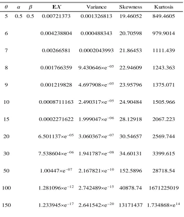
3.4 Effect of on the mean, variance, skewness and kurtosis

From Table 1 we note that: 1- 𝐸𝑋 decreases as 𝜃 increases.

2- The variance decreases as 𝜃 increases.

Table 1: Mean, variance, skewness and kurtosis.

   EX Variance Skewness Kurtosis

5 0.5 0.5 0.00721373 0.001326813 19.46052 849.4605

6 0.004238804 0.000488343 20.70598 979.9014

7 0.00266581 0.0002043993 21.86453 1111.439

8 0.001766359 9.430646e05 _{22.94609 1243.363}

9 0.001219828 4.697908e05 _{23.95796 1375.071}

10 0.0008711163 2.490317e05 _{24.90484 1505.966}

15 0.0002271622 1.999047e06 _{28.12918 2067.223}

20 6.501137e05 _3.060367e07 _{30.54657 2569.744}

30 7.538604e06 _1.941787e08 _{34.60131 3399.615}

50 1.00447e07 _2.167821e10 _{152.5896 28718.54}

100 1.281096e12 _2.742489e15 _{40878.74 1671225019}

150 1.233945e17 _2.641542e20 _{13171437 1.734868e}14

The moment generating function M.G.F.can be derived via Eq. (7) as

𝑚𝑟(𝑦) = 𝛤(1 + 𝑟𝛽−1) ∑ ∞

𝑑,𝑟,𝑚=0

𝜉_{𝑑,𝑟,𝑚}((𝑑+1)𝛼,𝑟)|_{[𝑟>−𝛽]},

where

[𝑡𝑟_/𝑟!]𝑉

𝑑+1 𝜉𝑚

((𝑑+1)𝛼,𝑟)

= 𝜉_{𝑑,𝑟,𝑚}((𝑑+1)𝛼,𝑟). The 𝑟𝑡ℎ incomplete moment of 𝑋 is defined by

𝜏_𝑟(𝑦) = ∫ 𝑦

−∞

𝑥𝑟𝑓(𝑥)𝑑𝑥.

We can write from (7)

𝜏_𝑟(𝑦) = 𝛾(1 + 𝑟𝛽−1, (𝑡−1)𝛽_{) ∑} ∞

𝑑,𝑚=0

By setting 𝑟 = 1,2,3 and 4 we get

𝜏1(𝑦) = 𝛾(1 + 𝛽−1, (𝑡−1)𝛽) ∑ ∞

𝑑,𝑚=0

𝜉_𝑑,𝑚((𝑑+1)𝛼,1)|_[1>−𝛽],

𝜏2(𝑦) = 𝛾(1 + 𝛽−2, (𝑡−1)𝛽) ∑ ∞

𝑑,𝑚=0

𝜉_𝑑,𝑚((𝑑+1)𝛼,2)|_[1>−𝛽],

𝜏₃(𝑦) = 𝛾(1 + 𝛽−3_{, (𝑡}−1₎𝛽_{) ∑} ∞

𝑑,𝑚=0

𝜉_𝑑,𝑚((𝑑+1)𝛼,3)|_[3>−𝛽],

and

𝜏₄(𝑦) = 𝛾(1 + 𝛽−4, (𝑡−1)𝛽_{) ∑} ∞

𝑑,𝑚=0

𝜉_𝑑,𝑚((𝑑+1)𝛼,4)|_[4>−𝛽].

3.5 Moments of residual life

The 𝑛𝑡ℎ moment of the residual life, say

𝐸(𝑋 − 𝑡)𝑛 = 𝑧𝑛(𝑡)|[𝑋>𝑡,𝑛=1,2,… ],

uniquely determines 𝐹(𝑥) . The 𝑛 th moment of the residual life of 𝑋 is given by

𝑧𝑛(𝑡) = 𝑅𝜃,𝛼,𝛽−1 (𝑡) ∫ ∞

𝑡

(𝑥 − 𝑡)𝑛𝑑𝐹𝜃,𝛼,𝛽(𝑥).

Therefore,

𝑧_𝑛(𝑡) =𝛾(1 + 𝑛𝛽

−1_{, (𝑡}−1₎𝛽₎

𝑅(𝑡) ∑

∞

𝑑,𝑚=0

𝜅_𝑑,𝑚((𝑑+1)𝛼,𝑛)|_{[𝑛>−𝛽]},

where

𝑞_𝑑+1𝜉_𝑚((𝑑+1)𝛼,𝑛) = 𝜅_𝑑,𝑚((𝑑+1)𝛼,𝑛), and

𝑉_𝑑+1∑ 𝑛

𝑟=0

(−𝑡)𝑛−𝑟₍𝑛

𝑟) = 𝑞𝑑+1

3.6 Moments of the reversed residual life

The 𝑛𝑡ℎ _{moment of the reversed residual life, say} 𝐸(𝑡 − 𝑋)𝑛 _{= 𝑍}

𝑛(𝑡)|[𝑋≤𝑡,𝑡>0,𝑛=1,2,… ],  we obtain

𝑍_𝑛(𝑡) = 𝐹_{𝜃,𝛼,𝛽}−1 (𝑡) ∫ 𝑡

0

(𝑡 − 𝑥)𝑛𝑑𝐹_{𝜃,𝛼,𝛽}(𝑥).

Then, the 𝑛𝑡ℎ moment of the reversed residual life of 𝑋 becomes

𝑍_𝑛(𝑡) =𝛾(1 + 𝑛𝛽

−1_{, (𝑡}−1₎𝛽₎

𝐹(𝑡) ∑

∞

𝑑,𝑚=0

𝛿_𝑑,𝑚((𝑑+1)𝛼,𝑛)|_{[𝑛>−𝛽]},

where

𝑉_𝑑+1∑ 𝑛

𝑟=0

(−1)𝑟₍𝑛

𝑟) 𝑡𝑛−𝑟 = 𝑙𝑑+1.

3.7 Order statistics

Suppose 𝑋1   :   𝑛, 𝑋2   :   𝑛, … , 𝑋𝑛   :   𝑛, is a random sample (R.S.) from the BHEW model. Let 𝑋_{𝑖   :   𝑛} denote the 𝑖𝑡ℎ _{order statistic. The P.D.F. of 𝑋}

𝑖   :   𝑛 is

𝑓_{𝑖   :   𝑛}(𝑥) = 𝐵−1_{(𝑖, 𝑛 − 𝑖 + 1) ∑}

𝑛−𝑖

𝑗=0

(−1)𝑗₍𝑛 − 𝑖

𝑗 ) 𝑓𝜃,𝛼,𝛽(𝑥)𝐹𝜃,𝛼,𝛽(𝑥)𝑗+𝑖−1.

(9)

Following the result 0.314 of Gradshteyn and Ryzhik (2000) for a power series raised to 𝑛 is a positive integer we have

∑ ∞ 𝑖=0 𝑐_𝑛,𝑖𝑢𝑖 _{= (∑} ∞ 𝑖=0 𝑎_𝑖𝑢𝑖₎ 𝑛

|_[𝑛≥1],

where 𝑐_𝑛,𝑖 (for 𝑖 = 1,2, … ) are the coefficients determined from the recurrence Eq. (with 𝑐_𝑛,0= 𝑎₀𝑛 )

(𝑖𝑎0)−1 ∑ 𝑖

𝑚=1

𝑎𝑚𝑐𝑛,𝑖−𝑚[𝑚(𝑛 + 1) − 𝑖] = 𝑐𝑛,𝑖.

The P.D.F. of the 𝑖𝑡ℎ _{order statistic of any BHEWmodel can be expressed as}

𝑓_{𝑖   :   𝑛}(𝜃,𝛼,𝛽)(𝑥) = ∑

∞

ℎ,𝑑=0

𝑏_ℎ,𝑑𝜋_ℎ+𝑑+1(𝑥),  (10)

where

𝑏_ℎ,𝑑 = 𝑛! (ℎ + 1)(𝑖 − 1)! (ℎ + 𝑑 + 1)−1_𝑑

ℎ+1∑

𝑛−𝑖

𝑗=0

(−1)𝑗𝑣_{𝑗+𝑖−1,𝑑}

(𝑛 − 𝑖 − 𝑗)! 𝑗!

and the quantities 𝑣𝑗+𝑖−1,𝑑 can be determined with and recursively for

𝑓_{𝑗+𝑖−1,𝑑} = (𝑑𝑑₀)−1 _∑

𝑑

𝑚=1

𝑑_𝑚 𝑣_{𝑗+𝑖−1,𝑑−𝑚}[ 𝑚(𝑗 + 𝑖) − 𝑑] .

4. For the BHEW model

5. 𝐸𝑋_{𝑖   :   𝑛}𝑞 = 𝛤(1 + 𝑞𝛽−1) ∑∞_{ℎ,𝑑,𝑚=0} 𝜉_{ℎ,𝑑,𝑚}(ℎ+𝑑+1,𝑞)|_{[𝑞>−𝛽]}, 6. where

7. 𝑏_ℎ,𝑑𝜉_𝑚(ℎ+𝑑+1,𝑞) = 𝜉_{ℎ,𝑑,𝑚}(ℎ+𝑑+1,𝑞).

8. Estimation

ℓ= ℓ(𝚿) = 𝑛 𝑙𝑜𝑔 𝛼 + 𝑛 𝑙𝑜𝑔 𝛽 + (𝛽 − 1) ∑ 𝑛 𝑖=1 𝑙𝑜𝑔𝑥_𝑖− ∑ 𝑛 𝑖=1 𝑥_𝑖𝛽 − ∑ 𝑛 𝑖=1

𝑥_𝑖𝛽+ (𝛼 − 1) ∑ 𝑛 𝑖=1 𝑙𝑜𝑔𝑧_𝑖+ ∑ 𝑛 𝑖=1 𝑙𝑜𝑔𝑞_𝑖  + ∑ 𝑛 𝑖=1 𝑙𝑜𝑔𝑠_𝑖 , where

𝑞_𝑖 = (1 − 𝑧_𝑖𝛼)𝜃−1_{/[1 − 𝑙𝑜𝑔(1 − 𝑧} 𝑖𝛼)]2,

𝑠_𝑖 = {𝜃[1 − 𝑙𝑜𝑔(1 − 𝑧_𝑖𝛼)] + 1} and

𝑧_𝑖 = [1 − 𝑒𝑥𝑝(−𝑥_𝑖𝛽)].

The components of the score vector is available if needed.

9. Applications

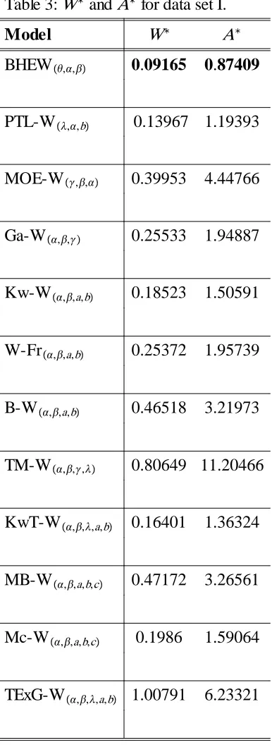
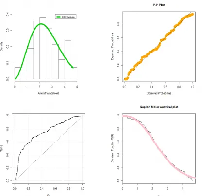
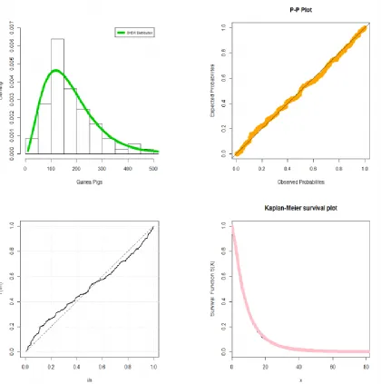
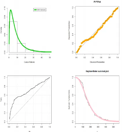
In this Section, we provide four applications to show empirically its potentiality. We consider the Cramér-Von Mises W* and the Anderson-Darling 𝐴∗ statistics. The computations are carried out using the R software. The M.L.E. and the corresponding standard errors (S.E.) (in parentheses) of the new model parameters are given in Tables 2, 4, 6, and 8. The numerical values of the W* _{and A}* _{are listed in Tables 3, 5, 7, and 9.} The estimated P.D.F., P-P plot, TTT plot and Kaplan-Meier survival plot of the four data sets of the proposed model are displayed in Figures 3, 4,5 and 6. These four data sets were used for fitting the Odd Lindley EW by Aboraya (2018).

Application 1

new distribution yields the lowest values of these statistics and hence provides the best fit to the two data sets.

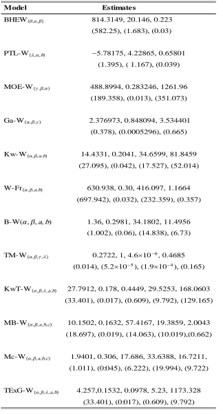
Table 2: M.L.E.s (S.E. in parentheses) for data set I.

Model Estimates

BHEW,, 814.3149, 20.146, 0.223 (582.25), (1.683), (0.03)

PTL-W,,b 5.78175, 4.22865, 0.65801 (1.395), ( 1.167), (0.039)

MOE-W,, 488.8994, 0.283246, 1261.96 (189.358), (0.013), (351.073)

Ga-W,, 2.376973, 0.848094, 3.534401 (0.378), (0.0005296), (0.665)

Kw-W_,,a,b 14.4331, 0.2041, 34.6599, 81.8459 (27.095), (0.042), (17.527), (52.014)

W-Fr,,a,b 630.938, 0.30, 416.097, 1.1664 (697.942), (0.032), (232.359), (0.357)

B-W(,,a,b) 1.36, 0.2981, 34.1802, 11.4956 (1.002), (0.06), (14.838), (6.73)

TM-W,,, 0.2722, 1, 4.6106, 0.4685 (0.014), (5.2105_{), (1.910}4_{), (0.165)}

KwT-W_,,,a,b 27.7912, 0.178, 0.4449, 29.5253, 168.0603 (33.401), (0.017), (0.609), (9.792), (129.165)

MB-W,,a,b,c 10.1502, 0.1632, 57.4167, 19.3859, 2.0043 (18.697), (0.019), (14.063), (10.019),(0.662)

Mc-W_,,a,b,c 1.9401, 0.306, 17.686, 33.6388, 16.7211, (1.011), (0:045), (6.222), (19.994), (9.722)

Table 3:WandAfor data set I.

Model W A

BHEW,, 0.09165 0.87409

PTL-W_{,,b} 0.13967 1.19393

MOE-W,, 0.39953 4.44766

Ga-W,, 0.25533 1.94887

Kw-W_,,a,b 0.18523 1.50591

W-Fr_{,,a,b} 0.25372 1.95739

B-W,,a,b 0.46518 3.21973

TM-W,,, 0.80649 11.20466

KwT-W_,,,a,b 0.16401 1.36324

MB-W,,a,b,c 0.47172 3.26561

Mc-W,,a,b,c 0.1986 1.59064

Figure 3: Estimated P.D.F., P-P plot, TTT plot and Kaplan-Meier survival plot for data set I.

Application 2

with corresponding densities (for x > 0 ) (for more details about these P.D.F.s see Aboraya (2018)).

Table 4: M.L.E.s (S.E. in parentheses) for data set II.

Model Estimates

BHEW,, 61.746, 45.807, 0.170

(157.0984), (7.291, (0.0544)

W, 9.5593, 1.0477

(0.853), (0.068)

TM-W,,, 0.1208, 0.8955, 0.0002, 0.2513

(0.024), (0.626), (0.011), (0.407)

MB-W,,a,b,c 0.1502, 0.1632, 57.4167, 19.3859, 2.0043

(22.437), (0.044), (37.317), (13.49), (0.789)

TA-W,,,, 0.1139, 0.9722, 3.0936105, 1.0065, -0.163

(0.032), (0.125), (6.106103_{), (0.035), (0.28)}

ETG-R,,, 7.3762, 0.0473, 0.0494, 0.118

(5.389),(3.965103_{), (0.036), (0.26)}

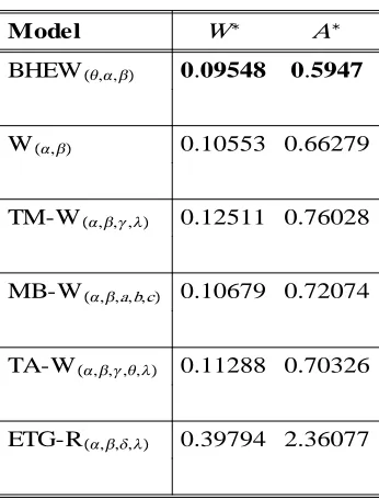
Table 5:WandAfor data set II.

Model W A

BHEW,, 0.09548 0.5947

W, 0.10553 0.66279

TM-W,,, 0.12511 0.76028

MB-W,,a,b,c 0.10679 0.72074

TA-W,,,, 0.11288 0.70326

Figure 4: Estimated P.D.F., P-P plot, TTT plot and Kaplan-Meier survival plot for data set II.

Application 3

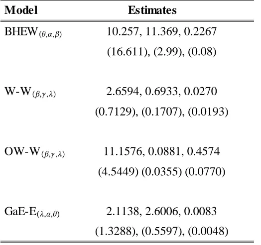
The second real data set corresponds to the survival times (in days) of 72 guinea pigs infected with virulent tubercle bacilli reported by Bjerkedal (1960). The data are: 72,74, 77, 10, 33, 44, 56, 59, 92, 93, 96, 107, 107, 108, 108, 100, 100, 102, 105, 108, 116, 120, 121, 122, 109, 112, 113, 115, 122, 124, 130, 146, 153, 159, 160, 134, 136, 139, 144, 163, 163, 168, 176, 183, 195, 196, 215, 216, 222, 230, 197, 202, 213, 231, 240, 245, 293, 327, 342, 251, 253, 254, 255, 278, 347, 361, 402, 171, 172,432, 458, 555.

Table 6: M.L.E.s (S.E. in parentheses) for data set III.

Model Estimates

BHEW,, 10.257, 11.369, 0.2267

(16.611), (2.99), (0.08)

W-W,, 2.6594, 0.6933, 0.0270

(0.7129), (0.1707), (0.0193)

OW-W,, 11.1576, 0.0881, 0.4574

(4.5449) (0.0355) (0.0770)

GaE-E,, 2.1138, 2.6006, 0.0083

(1.3288), (0.5597), (0.0048)

Table 7:WandAfor data set III.

Model W A

BHEW,, 0.0418 0.2792

W-W,, 0.1427 0.7811

OW-W,, 0.4494 2.4764

Figure 5: Estimated P.D.F., P-P plot, TTT plot and Kaplan-Meier survival plot for data set III.

Application 4: Glass fibers data

Table 8: M.L.E.s (S.E. in parentheses) for data set IV.

Model Estimates

BHEW,, 908.64, 21.127, 0.5

(577.313), (1.610), (0.057)

EWa,, 0.671, 7.285,1.718

(0.249), (1.707), (0.086)

T-Wa,, 0.5010, 5.1498, 0.6458

(0.2741), (0.6657), (0.0235)

OLL-W,, 0.9439, 6.0256, 0.6159

(0.2689), (1.3478), (0.0164)

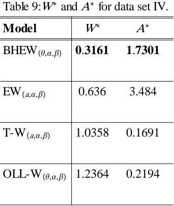
Table 9:W andA for data set IV.

Model W A

BHEW,, 0.3161 1.7301

EWa,, 0.636 3.484

T-Wa,, 1.0358 0.1691

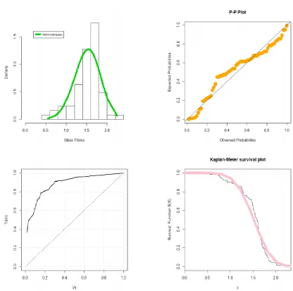
Figure 6: Estimated P.D.F., P-P plot, TTT plot and Kaplan-Meier survival plot for data set IV.

Based on Tables 3, 5, 7 and 9, the BHEW lifetime model provides adequate fits as compared to other Weibull models with small values for W* and A* . The BHEW lifetime model is better than the PTL-W, MOE-W, W-Fr, B-W, TM-W, KwT-W, Ga-W, Kw-W, MB-W, Mc-W and TExG-W models in modeling the failure times data, also the new model is much better than the TL-E, W, TM-W, MB-W, TA-W and ETG-R models in modeling cancer patients data, and much better than the OW-W and GaE-E models in modeling survival times of Guinea pigs. Finally, the proposed model is much better than the EW, T-W and OLL-W models in modeling glass fibers data. Also, Plots of estimated P.D.F., P-P, TTT and Kaplan-Meier survival given in Figures 3-6 supports these results.

10.Concluding remarks

models. We are also motivated to introduce the BHEW lifetime model since it exhibits increasing, decreasing and bathtub hazard rates. The BHEW model can be viewed as a mixture of the EW density. It can also be considered as a suitable model for fitting the left skewed, right skewed, symmetric, and unimodal data. We prove empirically the great importance and wide flexibility of the BHEW model in modeling four types of lifetime data, the new model provides adequate fits as compared to other Weibull models with small values for W* and A* so the new model is much better than other competitive model in modeling four data sets. The proposed lifetime model is much better than the Poisson Topp Leone-Weibull, Marshall Olkin extended-Weibull, Gamma-Weibull, Kumaraswamy-Weibull, Weibull-Fréchet, B-W, Beta-Weibull, Kumaraswamy transmuted-Weibull, transmuted modified-Weibull, transmuted exponentiated generalized Weibull, modified beta-Weibull and McDonald-Weibull models in modeling the failure times data. In modeling cancer patient's data, the new model is much better than the transmuted linear exponential, Weibull, Transmuted modified-Weibull, modified beta-Weibull, transmuted additive-Weibull and exponentiated transmuted generalized Rayleigh models. The BHEW model is much better than the Weibull-Weibull, Odd Weibull-Weibull and gamma exponentiated-exponential models in modeling survival times of Guinea pigs. Finally, the BHEW model is better than transmuted-Weibull, the exponentiated-Weibull and Odd Log Logistic-Weibull models in modeling glass fibers data.

References

1. Aboraya, M. (2018). A new flexible lifetime model with statistical properties and applications, Pak.j.stat.oper.res, forthcoming.

2. Almamy, J. A., Ibrahim, M., Eliwa, M. S., Al-mualim, S. and Yousof, H. M. (2018). The two-parameter odd Lindley Weibull lifetime model with properties and applications International Journal of Statistics and Probability, 7(4), 1927-7040.

3. Aryal, G. R., Ortega, E. M., Hamedani, G. G. and Yousof, H. M. (2017). The Topp Leone Generated Weibull distribution: regression model, characterizations and applications, International Journal of Statistics and Probability, 6, 126-141. 4. Alzaatreh, A., Lee, C. Famoye, F. (2013). A new method for generating

families of continuous distributions, Metron, 71, 63-79.

5. Bjerkedal, T. (1960). Acquisition of resistance in guinea pigs infected with different doses of virulent tubercle bacilli. American Journal of Hygiene, 72, 130-148.

6. Bourguignon, M., Silva, R.B. Cordeiro, G.M. (2014). The Weibull--G family of probability distributions, Journal of Data Science, 12, 53-68.

7. Brito, E., Cordeiro, G. M., Yousof, H. M., Alizadeh, M. and Silva , G. O. (2017). Topp-Leone Odd Log-Logistic Family of Distributions, Journal of Statistical Computation and Simulation, 87(15), 3040–3058.

Journal of Statistical Computation and Simulation, 88(3), 432-456.

9. Gradshteyn, I. S. and Ryzhik, I. M. (2000). Table of Integrals, Series and Products (sixth edition). San Diego: Academic Press.

10. Hamedani G. G. Yousof, H. M., Rasekhi, M., Alizadeh, M., Najibi, S. M. (2017). Type I general exponential class of distributions. Pak. J. Stat. Oper. Res., XIV (1), 39-55.

11. Korkmaz, M. C., Altun, E., Yousof, H. M. and Hamedani G. G. (2019). The Odd Power Lindley Generator of Probability Distributions: Properties, Characterizations and Regression Modeling, International Journal of Statistics and Probability, 8(2). 70-89.

12. Lee, C., Famoye, F. Olumolade, O. (2007). Beta-Weibull distribution: some properties and applications to censored data. Journal of Modern Applied Statistical Methods, 6, 17.

13. Maniu, A. I. and Voda, V. G. (2008). Generalized Burr-Hatke Equation as Generator of a Homogaphic Failure rate, Journal of applied quantitative methods, 3, 215-222.

14. Mudholkar, G. S. & Srivastava, D. K. (1993). Exponentiated Weibull family for analyzing bathtub failure-rate data. IEEE Transactions on Reliability, 42, 299-302.

15. Mudholkar, G. S., Srivastava, D. K. & Freimer, M. (1995). The exponentiated Weibull family: A reanalysis of the bus-motor-failure data. Technometrics, 37, 436-445.

16. Nadarajah, S., Cordeiro, G. M. Ortega, E. M. M. (2013). The exponentiated Weibull distribution: A survey, Statistical Papers, 54, 839-877.

17. Weibull, W. (1951). Statistical distributions function of wide applicability. J. Appl. Mech.-Trans, 18(3), 293-297.

18. Yousof, H. M., Afify, A. Z., Alizadeh, M., Butt, N. S., Hamedani, G. G. and Ali, M. M. (2015). The transmuted exponentiated generalized-G family of distributions, Pak. J. Stat. Oper. Res., 11 (4), 441-464.

19. Yousof, H. M., Afify, A. Z., Alizadeh, M., Butt, N. S., Hamedani, G. G. and Ali, M. M. (2015). The transmuted exponentiated generalized-G family of distributions, Pak. J. Stat. Oper. Res., 11 (4), 441-464.

20. Yousof, H. M., Afify, A. Z., Cordeiro, G. M., Alzaatreh, A., and Ahsanullah, M. (2017). A new four-parameter Weibull model for lifetime data. Journal of Statistical Theory and Applications, 16(4), 448 – 466.

Appendix

Figure 1: Plots of the BHEW P.D.F.