https://doi.org/10.5194/tc-13-1819-2019
© Author(s) 2019. This work is distributed under the Creative Commons Attribution 4.0 License.
Development of physically based liquid water schemes for
Greenland firn-densification models
Vincent Verjans1, Amber A. Leeson2, C. Max Stevens3, Michael MacFerrin4, Brice Noël5, and Michiel R. van den Broeke5
1Lancaster Environment Centre, Lancaster University, Lancaster, LA1 4YW, UK
2Lancaster Environment Centre, Data Science Institute, Lancaster University, Lancaster, LA1 4YW, UK 3Department of Earth and Space Sciences, University of Washington, Seattle, WA, USA
4Cooperative Institute for Research in Environmental Sciences, University of Colorado, Boulder, CO, USA 5Institute for Marine and Atmospheric research Utrecht, Utrecht University, Utrecht, the Netherlands Correspondence:Vincent Verjans ([email protected])
Received: 24 January 2019 – Discussion started: 13 February 2019 Revised: 29 May 2019 – Accepted: 4 June 2019 – Published: 9 July 2019
Abstract.As surface melt is increasing on the Greenland Ice Sheet (GrIS), quantifying the retention capacity of the firn layer is critical to linking meltwater production to meltwater runoff. Firn-densification models have so far relied on em-pirical approaches to account for the percolation–refreezing process, and more physically based representations of liquid water flow might bring improvements to model performance. Here we implement three types of water percolation schemes into the Community Firn Model: the bucket approach, the Richards equation in a single domain and the Richards equa-tion in a dual domain, which accounts for partiequa-tioning be-tween matrix and fast preferential flow. We investigate their impact on firn densification at four locations on the GrIS and compare model results with observations. We find that for all of the flow schemes, significant discrepancies remain with respect to observed firn density, particularly the density vari-ability in depth, and that inter-model differences are large (porosity of the upper 15 m firn varies by up to 47 %). The simple bucket scheme is as efficient in replicating observed density profiles as the single-domain Richards equation, and the most physically detailed dual-domain scheme does not necessarily reach best agreement with observed data. How-ever, we find that the implementation of preferential flow simulates ice-layer formation more reliably and allows for deeper percolation. We also find that the firn model is more sensitive to the choice of densification scheme than to the choice of water percolation scheme. The disagreements with observations and the spread in model results demonstrate that
progress towards an accurate description of water flow in firn is necessary. The numerous uncertainties about firn structure (e.g. grain size and shape, presence of ice layers) and about its hydraulic properties, as well as the one-dimensionality of firn models, render the implementation of physically based percolation schemes difficult. Additionally, the performance of firn models is still affected by the various effects affect-ing the densification process such as microstructural effects, wet snow metamorphism and temperature sensitivity when meltwater is present.
1 Introduction
melt-ing has become more widespread and intense on the Green-land Ice Sheet (GrIS), with annual total melt rates rising by 11.4 Gt yr−2 between 1991 and 2015 (van Angelen et al., 2014; van den Broeke et al., 2016). This meltwater perco-lates into the firn layer, where it can refreeze, run off or re-main liquid in temperate firn. Refreezing of liquid water in firn, known as internal accumulation, has an impact both on ice sheet mass balance and on heat fluxes from the surface to the ice sheet (van Pelt et al., 2012). As such, understanding physical processes in firn, including in particular the trans-port of liquid water, is becoming increasingly imtrans-portant in order to accurately constrain and predict the mass balance of the GrIS (van den Broeke et al., 2016).
Densification of dry firn is typically modelled as a func-tion of near-surface air temperature and accumulafunc-tion (Her-ron and Langway, 1980; Arthern et al., 2010; Li and Zwally, 2011; Simonsen et al., 2013; Morris and Wingham, 2014; Kuipers Munneke et al., 2015a, b). If applied to wet firn, these models are often modified to include a simplified rep-resentation of liquid water percolation, the bucket scheme, which assumes flow and refreezing through the firn column occur in a single time step (Simonsen et al., 2013; Kuipers Munneke et al., 2015b; Steger et al., 2017a). Observations have shown that, in reality, liquid water transport in firn is characterised by flow patterns that are heterogeneous in space and time (Pfeffer and Humphrey, 1996; Humphrey et al., 2012). Incorporation of liquid water schemes represent-ing such flow patterns would enable models to better repre-sent the transport of mass and heat through the firn; these schemes might also improve modelled densification in wet firn conditions (Kuipers Munneke et al., 2014; van As et al., 2016a; Meyer and Hewitt, 2017). Liquid water flow, how-ever, is a complex function of several properties and pro-cesses that are difficult to constrain by observations and, as a corollary, are difficult to represent in these models (e.g. pres-ence of impermeable ice layers, snow hydraulic properties, grain size, lateral runoff). The infiltration of water through firn can be partitioned between the progressive advance of a uniform wetting front through the pores, called matrix flow, and fast, localised, preferential flow (Waldner et al., 2004; Katsushima et al., 2013). This dual nature of water flow has been reported in observations of the firn layer of the GrIS, where preferential flow pathways come in the form of dis-crete vertical conduits and are crucial to effectively trans-port surface meltwater in deep subfreezing firn (Pfeffer and Humphrey, 1996; Parry et al., 2007; Humphrey et al., 2012; Cox et al., 2015). The detection of perennial firn aquifers (PFAs), in which large amounts (140 Gt) of liquid water are stored year-round in deep firn, further emphasises the impor-tance of firn hydrology on the GrIS mass balance (Forster et al., 2014; Koenig et al., 2014). Snow modellers have devel-oped liquid water schemes based on the Richards equation (RE) to simulate matrix flow (Hirashima et al., 2010; Wever et al., 2014; D’Amboise et al., 2017). The RE is a continuity equation describing water flow in unsaturated porous media
and is widely used in hydrological models. Recently, a pref-erential flow scheme has been included in the SNOWPACK model to account for heterogeneous percolation (Wever et al., 2016). Until now, however, such developments have not been implemented in firn-densification models.
In this study, we describe and compare liquid water schemes of different levels of physical complexity from snow models, and we apply these in combination with firn-densification models in order to evaluate the impact of the treatment of liquid water flow on modelled firn densification and temperature. We use the Community Firn Model (CFM) as the modelling framework for our study; the CFM is able to simulate numerous physical processes in firn and includes a large choice of governing formulations for densification. We use the common bucket approach and also develop schemes for liquid water flow in firn following physically based ad-vances in snow models (Wever et al., 2014, 2016; D’Amboise et al., 2017).
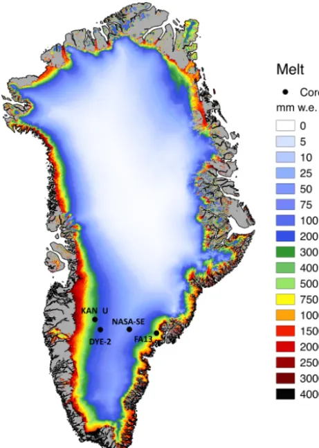
We simulate liquid water flow and firn densification start-ing from 1980 at four sites on the GrIS: DYE-2, NASA-SE, KAN-U and a PFA site (Fig. 1). These sites were chosen because they are collocated with recently drilled firn cores which allow a direct comparison of model results with servations. By comparing simulated firn densification to ob-servations at these sites, we investigate the sensitivity of the system to the choice of liquid water flow scheme and the sensitivity of the flow schemes to various parameterisations of firn structural properties. Finally, we perform simulations with a range of firn-densification formulae and assess the rel-ative importance of the choice of liquid water flow scheme to the choice of the underlying densification equation.
2 Firn model and data
In this study we use and further develop the CFM, an open-source firn-densification modelling framework. We refer the reader to Stevens (2018) for details and briefly summarise the main characteristics here. The CFM is one-dimensional and works in a Lagrangian framework; it is forced at its upper boundary by observed or modelled values for ac-cumulation, surface temperature, surface density, rain and snowmelt. The CFM includes many of the commonly used dry firn-densification schemes (e.g. Herron and Langway, 1980; Helsen et al., 2008; Arthern et al., 2010; Li and Zwally, 2011; Morris and Wingham, 2014; Kuipers Munneke et al., 2015b). We refer the reader to the original publications for details on the different densification schemes and briefly out-line the expressions used in our simulations in this section. 2.1 Dry firn-densification model
stud-Figure 1.Study site locations and mean annual melt rates (1958– 2017) from RACMO2.3p2.
ies of firn densification on the GrIS and also on polar ice caps (Gascon et al., 2014; Langen et al., 2017). This model is formulated so that densification is based on the overburden stress:
dρ dt =ρ
σ
η, (1)
whereρis the density of the firn (kg m−3),σis the stress due to weight of the upper layers (kg m−1s−2)andηis the snow viscosity (kg m−1s−1)following the parameterisation: η=f1f2η0
ρ cη
expaη(T0−T )+bηρ, (2)
where η0=7.62237 kg s−1m−1, aη=0.1 K−1,
bη=0.023 m3kg−1, T is the firn temperature (K) and
T0=273.15 K. The parameter cη is set to 358 kg m−3 as
suggested by van Kampenhout et al. (2017) when using Eq. (1) for polar firn. There are two additional correction factors, f1 andf2, depending on firn microstructural prop-erties. The factor f1 accounts for the presence of liquid water:
f1= 1
1+60θ, (3)
whereθ is the volumetric water content (m3m−3). In this study, we neglect the change in snow viscosity for grain sizes smaller than 0.3 mm by keeping the constant valuef2=4 (after Langen et al., 2017; van Kampenhout et al., 2017).
Several firn-densification equations have been derived and calibrated for the GrIS specifically. We favoured the use of Eq. (1) as our base case because (i) most of these cal-ibrated schemes were developed for dry firn densification, whereas the CROCUS formulation accounts for the pres-ence of liquid water explicitly; (ii) applying a percolation scheme in a stress-based densification model rather than in an accumulation-rate-based model ensures that the redistri-bution of mass associated with percolation will affect the densification appropriately; and (iii) the CROCUS densifica-tion scheme is currently used by the regional climate model (RCM) MAR and by the Community Earth System Model (CESM) to quantify firn densification on the GrIS (Fettweis et al., 2017; van Kampenhout et al., 2017).
2.2 Climatic forcing
To force the model at its upper boundary we use three-hourly skin temperature, melt, snowfall, rain and sublimation fields simulated by the latest version of the RACMO2 regional cli-mate model (RACMO2.3p2, Noël et al., 2018). This model has a 5.5 km horizontal resolution grid and has been explic-itly adapted for use over the polar ice sheets. Discrepan-cies between the climatic forcing and the real climatic his-tory can bias the firn models’ results. For the areas of our study sites (Sect. 2.4), we provide detailed statistical com-parisons between RACMO2.3p2 output and available obser-vations (see Sect. S1 in the Supplement). We further refer to Noël et al. (2018) for more discussion about the perfor-mance of RACMO2.3p2 on the GrIS scale and related uncer-tainties. Additionally, Ligtenberg et al. (2018) have demon-strated the impact of recent developments in RACMO2.3p2 on firn modelling, mostly yielding improvements in mod-elled densification.
If the solid input rate (snowfall – sublimation) is negative over a time step, the CFM treats it as a corresponding mass loss in the surface layer; liquid water is evaporated before solid mass gets sublimated. The temperature of a newly ac-cumulated snow layer is defined as the skin temperature at that time step. Deep firn temperatures in the model are thus mostly determined by the mean surface temperature applied during the spin-up process (Sect. 2.5) together with latent heat release through refreezing. We use a Neumann bound-ary condition for the temperature at the bottom of the domain and use a 250 m deep column to account for the large thermal mass of the ice sheet during the transient run.
ks, a function of density following Anderson (1976): ks=0.021+2.5
ρ
1000
2
. (4)
Another boundary condition is the density of every fresh snow layer deposited at the surface. To reduce the sources of possible uncertainties, we simply use a constant and site-specific surface density according to the surface value of the drilled firn cores instead of a parameterised formulation (see Sect. 2.4).
2.3 Grain size
The temporal evolution of grain size in firn is poorly under-stood and observational constraints are scarce. However, the grain size is a key variable for the RE, and the flow schemes used in this study thus require an initial grain size and a grain growth rate. For the former, we use the empirical formulation of Linow et al. (2012) derived from observations of snow samples from Antarctica and Greenland:
r0=(b0+b1(Tav−T0)+b2b˙ ρi ρw
), (5)
whereρi is the ice density (917 kg m−3);ρw is that of liq-uid water (1000 kg m−3);b˙is the mean annual accumulation rate (m w.e. yr−1);Tav the mean annual surface temperature (K); andb0,b1andb2are calibration parameters taking the values 0.781 m, 0.0085 m K−1and−0.279 yr (m w.e.)−1 re-spectively.
For grain growth rate, the relationship proposed by Kat-sushima et al. (2009) is applied:
dr dt =
1 8r2109min
2
π
1.28 10−8+4.22 10−10 θweight,% 3
,
6.9410−8i,
(6) whereris the grain radius (m) andθweight,%is the mass liquid water content expressed in percent and is thus related to θ (see Eq. 3):
θweight,%=100
θ ρw(ρi−ρ) ρiρ
. (7)
Equation (6) combines a wet snow metamorphism formula and a higher limit of growth rate of ice particles, both derived from laboratory measurements.
To study the sensitivity of the model to the grain-size im-plementation, we also use an alternative option based on the approach for West Antarctic firn of Arthern et al. (2010); the grain radius in newly deposited layers (r0)has the constant value of 0.1 mm and the grain growth rate is formulated as
dr dt =
1 2rkgexp
−E g RT
, (8)
where Eg is the activation energy for grain growth (42.4 kJ mol−1),R is the gas constant (8.314 J mol−1K−1) andkga parameter that takes the value 1.3×10⁻⁷m2s−1. Note that Eq. (8) does not take the impact of liquid water presence on firn metamorphism into account.
2.4 Study sites
We perform simulations at four study sites in the perco-lation zone of the GrIS where the availability of well-documented firn cores allows for model–observation com-parisons: NASA-SE, DYE-2, KAN-U and FA13 (peren-nial firn aquifer) (Fig. 1). NASA-SE (66.48◦N, 42.50◦W; 2372 m a.s.l.) is located in the upper part of the percola-tion zone with a mean annual temperature of −20◦ and relatively low melt rates (50 mm yr−1). DYE-2 (66.48◦N, 46.28◦W; 2126 m a.s.l.) is a slightly warmer site (T
av= −18◦), and melt is about 3 times greater than at NASA-SE (150 mm yr−1). KAN-U (67.00◦N, 47.03◦W; 1838 m a.s.l.) is near the equilibrium line altitude and has warmer temper-atures (Tav= −8◦) and significant melting (280 mm yr−1). FA13 (66.18◦N, 39.04◦W; 1563 m a.s.l.; Tav= −13◦) is a location known to contain a firn aquifer (Forster et al., 2014). The persistence of deep saturated layers year-round is due to the coupling of high melt rates (587 mm w.e. yr−1)with high accumulation rates (1002 mm w.e. yr−1)(Kuipers Munneke et al., 2014). Multiple firn core density data exist, a large part of which are available in the SUMup dataset (Mont-gomery et al., 2018). The selection of these four particular sites is motivated by their variety in climatic and glacio-logical conditions: a cold site with low melt rates, a cold site with high melt rates, a site close to the equilibrium line with substantial refreezing and a site with the presence of a firn aquifer. We perform transient firn-model simulations for each site until the date that a core was drilled. The cores at NASA-SE and DYE-2 were drilled in spring of the years 2016 and 2017 respectively, as part of the FirnCover project. The cores at KAN-U (Machguth et al., 2016) and at FA13 (Koenig et al., 2014) were drilled in spring 2013. The firn-temperature measurements were given in the sources men-tioned for the density data, except at KAN-U for which it comes from the collocated automatic weather station over-seen by the Programme for Monitoring of the Greenland Ice Sheet (PROMICE) (van As et al., 2016b). The fixed surface densities for DYE-2, NASA-SE, KAN-U and FA13 are 325, 240, 325 and 365 kg m−3respectively and were taken in ac-cordance with the surface density of the drilled cores. 2.5 Spin-up and domain definition
cli-mate because it predates the onset of the general warming of Greenland and the subsequent increase in surface melt. We iterate over the reference climate until 70 m w.e. of snow has been accumulated, which ensures the entire firn column is refreshed. The number of iterations over the reference cli-mate is thus site-specific. This spin-up process starts from an analytical solution for the density profile (Herron and Lang-way, 1980) with temperatures corrected to account for latent heat release by refreezing (Reeh, 2008). During the spin-up process we use the simple bucket approach, and the more ad-vanced flow schemes, detailed in the next section, are turned on only at the end of the spin-up for the transient simulation. This is because using the advanced schemes over long peri-ods is computationally expensive. The domain on which the flow calculations are applied is a subset of the entire CFM do-main; this sub-domain is defined each time the flow routine is called in the transient run. The bottom of the sub-domain is defined as the depth below which all layers have density higher than the pore close-off value (830 kg m−3), because infiltration of liquid water becomes negligible at this point. The thickness of the layers deposited in every three-hourly time step determines the vertical resolution, and we apply a merging process only to individual layers less than 2 cm thick (see Sect. S2.8).
3 Liquid water schemes
The water flow schemes are added to the dry-densification model detailed in Sect. 2.1 and are thus also effectively one-dimensional, representing no lateral exchange of heat and mass although lateral runoff is used as a mass sink. In this section, we present the three different flow schemes that we implement in the CFM: (1) the bucket method (BK), (2) a single-domain Richards equation scheme (R1M) and (3) a dual-permeability Richards equation scheme (DPM). Because of its robustness and ease of implementation, BK is the current state of the art in firn-densification models that are interactively coupled to regional climate models. R1M is used in several stand-alone snow models to describe water flow (Hirashima et al., 2010; Wever et al., 2014; D’Amboise et al., 2017), and DPM is entirely based on the scheme im-plemented in the snow model SNOWPACK (Wever et al., 2016), where dual-permeability means that separate domains for matrix flow and preferential flow coexist with liquid wa-ter exchanged between these domains.
3.1 Bucket model
The bucket percolation scheme is commonly used to account for the vertical transport of meltwater in firn models, though the precise form of its implementation is variable. Each layer in the model can refreeze meltwater according to its “cold content”, i.e. the energy required to raise the temperature of the layer to the melting point. Starting from the surface,
the meltwater may percolate through successive layers, thus allowing for refreezing at depth. Meltwater is progressively depleted due to refreezing and retention according to each layers’ water-holding capacity, which is the part of the water that is stored in some of the available pore space and not sub-ject to vertical transfer. The water-holding capacity acts as an approximation of the effect of capillary forces on water re-tention. Percolation proceeds until all the meltwater is stored (refrozen or retained) or until it reaches a layer with a density exceeding the impermeability threshold (780–830 kg m−3), at which point all the water in excess is instantly treated as lateral runoff. The BK thus requires two parameters: the water-holding capacity and the impermeability threshold. We test two possibilities for the former and three for the latter. The water-holding capacity can be prescribed by the calcula-tions of Coléou and Lesaffre (1998) for the mass proportion of water in a firn layer,Ww:
Ww=0.057 ρi−ρ
ρ . (9)
This mass proportion is then converted to the water-holding capacity,θh:
θh= Ww (1−Ww)
ρ ρi ρw(ρi−ρ)
. (10)
Using constant values of the water-holding capacity is also common practice (Reijmer et al., 2012; Steger et al., 2017a). Our base case scenario uses a fixedθhat 0.02, or 2 % of the pore space available for liquid water retention. This low value assumes effective downward percolation and is meant to ac-count for vertical preferential flow (Reijmer et al., 2012). For that reason, we consider this as a good basis for comparison with the DPM that explicitly accounts for such flow.
We test three values for the impermeability threshold; these were selected in accordance with Gregory et al. (2014), who tested firn permeability of Antarctic samples in a lab and reported that impermeability can occur over density val-ues ranging from 780 to 840 kg m−3. We thus take our three test values to be 780, 810 and 830 kg m−3, respectively the lower bound and middle of this range and a commonly used value of pore close-off density.
3.2 Richards equation
Vertical movement of water in a variably saturated porous medium can be described by the one-dimensional version of the RE:
∂θ ∂t −
∂ ∂z
K (θ )
∂h
∂z+1
=0, (11)
includes the “suction head”, i.e. the suction force exerted at the surface of individual grains.
A water-retention curve describes the relationship be-tween θ and h required by Eq. (11). We use the van Genuchten (1980) model, which is typically applied in stud-ies of liquid water flow through snow (Jordan, 1995; Hi-rashima et al., 2014; Wever et al., 2014; D’Amboise et al., 2017):
θ=θr+(θsat−θr)
(1+ α|h|n−m
Sc , (12)
whereθris the residual water content (m3m−3)andθsat is the volumetric liquid water content at saturation (m3m−3). Sc is a correction coefficient following Wever et al. (2014). The parameters α,n andmare tuning coefficients, with α being related to the maximum pore size and n andm be-ing related to the pore size distribution. These three parame-ters, referred to as the van Genuchten parameparame-ters, are specific to the modelled porous medium and for snow; a common approach is to use the parameterisation developed by Yam-aguchi et al. (2012) in a laboratory study:
α=4.4 106ρ 2r
−0.98
, (13)
n=1+2.7 10−3ρ 2r
0.61
, (14)
m=1−1
n. (15)
Yamaguchi et al. (2012) measured the water-retention curve for a range of grain radii (0.025 to 2.9 mm) and densities (361 to 636 kg m−3)in different snow samples by using a gravity drainage column method.
The porosity is the part of the volume not occupied by the solid matrix and, in the case of firn, is defined as
P =1− ρ ρi
. (16)
The volumetric liquid water content at saturation is propor-tional to the porosity (Wever et al., 2014):
θsat=P ρi ρw
. (17)
Note that water is not assumed to fill the entire pore space in saturated conditions and the correction factor ρi
ρw included in Eq. (17) accounts for the required space to allow the liquid water to freeze. It is reasonable to use this correction factor since Yamaguchi et al. (2010) found that trapped air still oc-cupies 10 % of the porosity in saturated snow.
The parameterθsatthus represents the pore space available for liquid water, and from there we can define the effective saturation as
Se= θ−θr θsat−θr
, (18)
and Se must be bounded between 0 and 1. In completely dry layers, a zero effective saturation would lead to infinite val-ues in the head pressure calculation, and, thus, we use a nu-merical adjustment to avoid this happening (see Sect. 2.3). The residual water contentθris defined as the amount of liq-uid water that cannot be removed by gravity as it is held by capillary tension at the surface of the solid grains. Follow-ing Yamaguchi et al. (2010), a constant value ofθr=0.02 can be taken, but, in case of refreezing,θcan approach zero andθrmust be adjusted accordingly. We takeθrfollowing a piecewise function:
θr=min [0.02,0.9θ]. (19)
The numerical requirement of an effective saturation value strictly greater than zero causes the persistence of very low flow rates, even for liquid water contents close to the residual water content. Over long time periods, layers cannot hold any residual water content and eventually dry out under the effect of gravity. By taking the coefficient 0.9 in Eq. (19) instead of 0.75 used in snow models (Wever et al., 2014; D’Amboise et al., 2017), we partially reduce this effect because this lowers the effective saturation value Se for any value of volumetric water contentθapproaching zero.
The hydraulic conductivity (K (θ )) is the ability of the fluid to flow through the porous medium under a certain hydraulic gradient dependent on pressure head and gravity. Thus,K (θ )depends on the effective saturation and on the properties of both the porous medium and the fluid; fluid flow is enhanced in highly saturated layers. The hydraulic con-ductivity is described by the van Genuchten–Mualem model (Mualem, 1976; van Genuchten, 1980):
K (θ )=Ksat Se1/2h1−1−Sem1 mi2
, (20)
where Ksat is the hydraulic conductivity in saturated condi-tions (Se=1). For the case of water flow through snow, it has been inferred using three-dimensional images of the mi-crostructure by Calonne et al. (2012) as
Ksat=3.0r2exp(−0.013ρ)
g ρw µ
, (21)
implementation completely describes R1M and provides the basis of DPM, further detailed in the next section.
Details of the numerical implementations that are required to maintain stability and to improve computational efficiency for the RE calculations are discussed in the Supplement. 3.3 Dual-permeability model
Physical models of preferential flow in snow are still scarce (Hirashima et al., 2014; Wever et al., 2016). In this section, we explain how the SNOWPACK dual-permeability model (Wever et al., 2016) is implemented in the CFM. The firn column is separated into two domains and water flow in both is governed by the RE (Sect. 3.2). We defineF as the pore space allocated to the preferential flow domain and accord-ingly 1−F as the pore space for the matrix flow domain. Wever et al. (2016) used a grain-size dependence forF, but their regression was performed on only four data points mea-sured in idealised snow laboratory conditions (Katsushima et al., 2013). The experimental grain sizes ranged from 0.1 to 0.8 mm and the water input from 480 to 550 mm per day, which is not representative of firn conditions in Greenland (Figs. 1 and 2). Moreover, due to the typical grain-size ranges in firn (Gow et al., 2004; Lyapustin et al., 2009), the model would regularly be forced to use for F the minimal value for numerical stability implemented in SNOWPACK. To deal with this uncertain parameter but still retain fidelity with re-spect to the SNOWPACK implementation, we favour the use of a constant value based on observations in natural snow. Marsh and Woo (1984) and Williams et al. (2010) reported that rapid flow paths occupy respectively 22 % and 5 % to 30 % of the area, and we thus fix the valueF =0.2. The ex-tension of the preferential flow area within the snowpack is very likely to be a function of grain size and meltwater in-flux, and these dependencies are still uncertain (Avanzi et al., 2016). The value ofF thus determines the value of the satu-rated liquid water contentθsatin both domains, and, instead of Eq. (17), we write
θsat,m=(1−F )P ρi ρw θsat,p=F P
ρi ρw
, (22)
where from hereon, the subscripts m and p stand for ma-trix and preferential flow domain respectively. Equation (22) shows that the volumetric water content in the preferential flow domain is smaller than that in the matrix flow domain. All the input of meltwater is added to the matrix flow domain. For the regulation of the exchange of water between domains, we also closely follow the transfer processes of SNOWPACK (Wever et al., 2016) which are executed at the same 15 min time step. We briefly summarise the transfer processes below. Water from the matrix flow domain can enter the preferen-tial flow domain of the layer below if the pressure head in the layer reaches the water entry suction,hwe, of the underlying
layer. The parameter can be expressed as (Katsushima et al., 2013; Hirashima et al., 2014; Wever et al., 2016)
hwe=0.0437(2r)−1+0.01074. (23)
The amount of water transferred into the preferential flow domain equals the amount of water in excess ofhwe. If af-ter the transfer Se in the matrix flow domain still exceeds Se in the preferential flow domain of the underlying layer, their respective Se’s are equalised by transferring the appro-priate amount of water from the overlying matrix flow do-main to the underlying preferential flow dodo-main. In addition, in every individual firn layer where Se in the matrix flow domain exceeds Se in the preferential flow domain, matrix and preferential Se’s are equalised by transferring water from the matrix flow domain to the preferential flow domain. This serves to avoid the presence of horizontal pressure gradients in wet snow.
Water can flow from the preferential flow domain to the matrix domain by two processes. The first process is when the saturation in the preferential flow domain exceeds a threshold value2. Wever et al. (2016) determined2by tun-ing its value to best match observations. When this threshold is reached, the amount of water corresponding to the cold content of the layer flows back into the matrix domain. If there is still water in excess of the threshold in the prefer-ential flow domain, saturation in both domains is set equal to one another. The second process simulates the heat flow from the preferential flow domain (at the melting point) to the colder surrounding matrix domain. Instead of transferring sensible heat, this process allows liquid water and its inher-ent latinher-ent heat to be exchanged to account for a theoretical heat flow,Q, and thus approximating Fourier’s law:
Q=ks
(T−T0) q
1+F
2π −
q
F π
. (24)
This formulation assumes a linear horizontal temperature gradient in the matrix and a circular shape of the preferen-tial flow path’s perimeter. From Eq. (24), the corresponding water transfer is calculated as
1θp→m= 2N
√
π F Q 1t15 Lfρw
, (25)
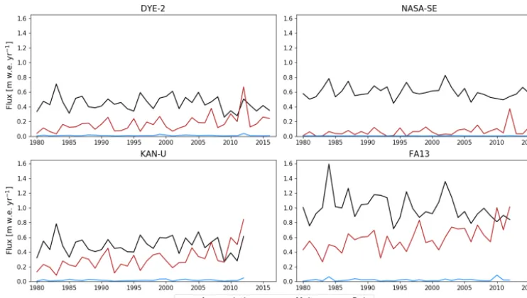
Figure 2.Annual surface mass fluxes from RACMO2.3p2 at the study sites (1980–drilling date).
subfreezing firn column, which can be up to 70 m thick in some areas of the GrIS. Therefore, we use the smallest non-zero value ofNtested by Wever et al. (2016), and the param-eters2andN are fixed to 0.1 and 0.2 m−2respectively.
The hydraulic conductivity of ice layers is not artificially set to zero in the preferential flow domain as it is in the ma-trix flow domain. Preferential flow thus provides a way for water to flow through an ice layer, reproducing observations that ice layers are not totally impermeable barriers and can lead to localised piping events (Marsh and Woo, 1984; Pfef-fer and Humphrey, 1998; Williams et al., 2010; Sommers et al., 2017). An exception for this is the bottom of the domain: as preferential flow is stopped at the last layer, it does not percolate through the solid ice.
3.4 Additional processes in the single- and dual-domain schemes
3.4.1 Refreezing process
In R1M and DPM a cold content is calculated for every firn layer, similarly to BK (Sect. 3.1), and refreezing in both flow schemes is executed at the 15 min time step (equivalent to the time step of the transfer processes of DPM, Sect. 3.3).
When refreezing occurs, every layer freezes the maximum of its liquid water content that its cold content allows. For numerical reasons, refreezing cannot dry out a layer com-pletely; instead, a very low value of liquid water remains in every layer (see Sect. S2.3). The refrozen water densifies the firn layer and modifies its hydraulic properties. The remain-ing liquid water is still subject to flow and infiltrates deeper into the firn column.
In DPM, refreezing is restricted to the matrix flow domain (see Sect. S2.7). In the preferential flow domain, liquid water
can percolate through cold layers, as has been observed in field studies on the GrIS (e.g. Pfeffer and Humphrey, 1996; Humphrey et al., 2012). For this liquid water to refreeze, it first has to be transferred back to the matrix flow domain. Preferential flow thus provides a way for liquid water to by-pass cold firn layers and subsequently to infiltrate deeper lay-ers.
3.4.2 Aquifer development and lateral runoff
In R1M and DPM, lateral runoff in the firn column is simulated using the parameterisation of Zuo and Oerle-mans (1996):
dRu dt =
Lexcess τRu
, (26)
τRu=c1+c2exp(−c3S), (27) where Ru is the amount of meltwater that runs off (m),Lexcess is the excess of liquid water amount with respect to the resid-ual water content (m) andτRuis a characteristic runoff time (s). The constantsc1, c2 andc3 are parameters derived by comparison with observations by Zuo and Oerlemans (1996) for the GrIS, andSis the surface slope. The meltwater input is immediately treated as lateral runoff if the surface layer is an impermeable ice layer or if it is saturated.
(Poinar et al., 2017), and possibly hydrofracture and rapid drainage events (Koenig et al., 2014). Miller et al. (2018) found discharge rates within the firn aquifer to be 4.3× 10⁻⁶m s−1by borehole dilution tests in the field. We tested this approach in our model by applying this value as a con-stant discharge rate for aquifers formed in our simulations. We found however that, using this approach, an aquifer was not sustained; suggesting that such discharge rates must be dependent on the total amount of water within the aquifer and are likely temporally variable. To account for drainage pro-cesses and yet allow the formation of an aquifer, we there-fore limited the amount of water stored in the firn aquifer to 1.65 m w.e., i.e. the water level measured in the field by Koenig et al. (2014). In firn aquifers forming at the bottom of the firn column, the saturation in both domains is equalised and the model does not perform flow calculation in this low-est part of the domain (see Sect. S2.5).
3.5 Investigating model sensitivity
In Sects. 2 and 3, we highlight several factors influenc-ing BK, R1M and DPM. For each of the schemes, we analyse results generated using three possible impermeabil-ity thresholds: 780 kg m−3(ip780), 810 kg m−3 (ip810) and 830 kg m−3(ip830). This provides a way to compare the sen-sitivity of the simple BK and of the physically based schemes (R1M and DPM) to a common parameter. For BK, we try two different formulations of the water-holding capacity: con-stant at 0.02 (wh02) and according to the parameterisation of Coléou and Lesaffre (1998), Eq. (9) (whCL). For R1M and for DPM, we test two different grain-size implementa-tions: the Linow et al. (2012) surface grain-size calculation, Eq. (5), coupled to the Katsushima et al. (2009) grain growth rate, Eq. (6) (grLK); and the grain-size implementation of Arthern et al. (2010), Eq. (8) (grA). It is important to exam-ine model sensitivity to the grain-size variable as almost all the hydraulic parameters of the RE depend on it. The differ-ent sensitivity tests are summarised in Table 1.
4 Results
In this section, we describe and discuss the model perfor-mance at each of the four sites tested (DYE-2, NASA-SE, KAN-U and FA13). We begin by comparing BK, R1M and DPM in a base case parameterisation: BK wh02 ip810, R1M grLK ip810 and DPM grLK ip810 respectively. Then, we perform various tests to investigate the sensitivity of the flow schemes to variations in their parameter values. We refer to ice layers as layers with a density value exceeding the im-permeability threshold in the model and to liquid water input as the total of meltwater and rain influx. The DPM approach features two tuning parameters,N and2. Model results and depth–density profiles were found to be weakly sensitive to the value ofNand2, and so we omit consideration of these
from the remainder of our study. Results of simulations and observations are inter-compared based on the firn air content (FAC; the depth integrated porosity in a firn column) over the top 15 m of firn and the temperature at 10 m depth. Com-paring the modelled FAC and 10 m depth temperature val-ues with observed data depicts the ability of the tested mod-els to reproduce the bulk condition of the upper firn column. We also qualitatively assess the degree to which the models to form a realistic ice-layer distribution and depth–density profile. One would not expect simulated values of either to match observations precisely given the high spatial variabil-ity of firn structure (Marchenko et al., 2017), but it is indica-tive of the models’ performance in reproducing heterogeneity in firn density.
4.1 DYE-2
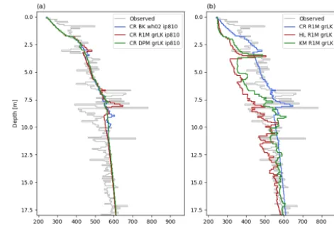
DYE-2 has a typical liquid water input between 0.1 and 0.3 m w.e. yr−1(Fig. 2), which is moderate in the context of our study sites. The extreme melt year of 2012 (Nghiem et al., 2012) is an exception, with an estimated input of more than 0.7 m w.e. Using BK, almost all of this meltwater re-freezes locally and runoff is close to zero (Table 2) until the 2012 summer when ice layers (ρ≥810 kg m−3)start form-ing in the top 2 m (Fig. 3a). Runoff increases in the subse-quent years because meltwater reaches these ice layers. In R1M and DPM, small amounts of runoff occur between 1980 and 2011 due to the lateral runoff implementation, Eq. (26). Beginning in summer 2004, some ice layers start to form in R1M (Fig. 3b) due to the refreezing of water held close to the surface by capillary forces. Over the 2012 summer, surface layers are progressively melted, bringing ice layers closer to the surface. The ponding and refreezing of water on the top ice layer allows it to thicken. This then acts as an imperme-able barrier to vertical percolation from 2012 onwards, re-sulting in a more than 6-fold increase in runoff (Table 2). In contrast, runoff remains low in DPM, in which several ice layers form in the upper firn as early as summer 1996 (Fig. 3c). These ice layers generally form deeper than 2 m due to more effective water transfer from the near-surface to lower layers; preferential flow provides a path for ponding meltwater in the matrix flow domain to bypass ice layers and continue to percolate vertically, thus maintaining low runoff amounts. Preferential flow brings part of the 2012 meltwater to depths greater than 12 m. For each flow scheme, the mod-elled FAC underestimates the observed value by 4 %–16 %. This can partly be attributed to the tendency of the CROCUS scheme to slightly overestimate densification rates in the up-per part of polar firn (Gascon et al., 2014). FAC is underes-timated more strongly in DPM (16 %) than in BK and R1M (4 %) because in DPM the deeper firn is not isolated from surface meltwater percolation (Table 2).
Table 1.Summary of the sensitivity tests.
Bucket model (BK) Single-domain RE (R1M) Dual-permeability RE (DPM)
Impermeability Water-holding Impermeability Grain-size Impermeability Grain-size threshold (ip) capacity (wh) threshold (ip) formulation (gr) threshold (ip) formulation (gr)
780 810 830 0.02 CL 780 810 830 LK A 780 810 830 LK A
Table 2.Model outputs at DYE-2 site. A slash indicates no data.
Refreezing/ Refreezing/ Runoff/ Runoff/ Top 15 m FAC (m) T 10 m (K)
inflow inflow inflow inflow (anomaly vs. (anomaly vs.
(1980–2011) (2012–2016) (1980–2011) (2012–2016) observations) observations, K)
BK (wh02 ip810) 0.96 0.67 0.01 0.31 5.01 (−4 %) 260.88 (+0.21)
R1M (grLK ip810) 0.91 0.63 0.05 0.35 4.99 (−4 %) 260.27 (−0.40)
DPM (grLK ip810) 0.95 0.95 0.02 0.03 4.38 (−16 %) 263.39 (+2.72)
Observations – – – – 5.21 260.67
DPM (grLK ip780) 0.95 0.96 0.02 0.02 4.39 (−16 %) 263.45 (+2.78)
BK (wh02 ip780) 0.96 0.60 0.02 0.38 5.15 (−1 %) 260.68 (+0.01)
BK (whCL ip810) 0.92 0.62 0.05 0.36 5.21 (+0 %) 259.40 (−1.27)
BK (wh02 ip830) 0.97 0.68 0.00 0.31 4.96 (−5 %) 260.98 (+0.31)
R1M (grA ip810) 0.83 0.59 0.14 0.38 5.19 (−0 %) 259.64 (−1.03)
DPM (grA ip810) 0.93 0.93 0.04 0.05 4.40 (−16 %) 263.08 (+2.41)
HL DPM (grLK ip810) 0.95 0.96 0.02 0.02 4.16 (−20 %) 263.78 (+3.11)
KM DPM (grLK ip810) 0.95 0.95 0.02 0.02 3.35 (−36 %) 262.74 (+2.07)
HL R1M (grLK ip810) 0.90 0.72 0.07 0.26 4.65 (−11 %) 260.41 (−0.26)
KM R1M (grLK ip810) 0.91 0.75 0.06 0.23 4.00 (−23 %) 260.26 (−0.41)
but no configuration is able to qualitatively reproduce the strong variability in density observed. For example, numer-ous high-density layers separated by much-lower-density in-tervals are clear in the observations. Regardless of the flow scheme, only a few ice layers are formed in the model and these tend to be confined to the upper 6 m, which has been affected by the higher melting rates of the recent years. In older firn deposited under lower-melt conditions, the num-ber of density peaks and their amplitude is underestimated even more strongly. Several ice layers are observed in the 10–20 m depth range; only DPM simulates the presence of ice layers here.
The three flow schemes lead to significantly different firn thermal conditions. The temperatures at 10 m depth of BK and R1M agree well with observations (+0.2 and−0.4 K). In contrast, 10 m temperature is strongly overestimated in DPM (+2.7 K) because it allows percolation at depth, subsequent refreezing and latent heat release. The summer 2012 perco-lation raises the 10 m depth temperature to within a few de-grees of melting using DPM. Since the DPM method seems to exaggerate deep percolation, we tested a lower imperme-ability threshold (DPM grLK ip780) which should favour the formation of shallow ice layers, the ponding of water in the matrix flow domain, more lateral runoff and colder temperatures at depth. The ice layers do form slightly ear-lier in the melt seasons but are not noticeably shallower than
in DPM ip810. The partitioning between runoff and refreez-ing is barely affected and the 10 m temperature bias remains (Table 2).
The BK method gives a density profile closer to R1M than to DPM. In order to mimic the behaviour of DPM we increase the impermeability threshold in BK (BK wh02 ip830) to make it more effective in transporting water ver-tically; however, model results are only weakly affected by this change (Table 2). We also modify the water-holding ca-pacity in BK according to the parameterisation of Coléou and Lesaffre (1998) (BK whCL ip810) which allows more water to be retained in the low-density layers close to the surface. Ice layers appear earlier in the simulation and at shallower depths (Fig. 3d). This increases the amount of runoff in BK whCL ip810 with respect to BK wh02 ip810 (+4 % of the water input over the entirety of the transient model run); how-ever, in the surface layers, where high amounts of water are retained, refreezing dominates. As a result, much less water percolates to the deeper firn and there is less refreezing and latent heat release. All of this leads to a significantly higher FAC (+4 %) and colder 10 m temperature (−1.5 K) relative to BK wh02 ip810.
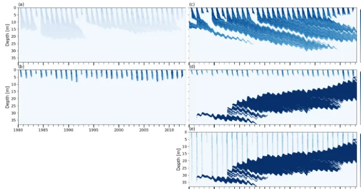
Figure 3.Modelled firn density at DYE-2.(a)BK wh02 ip810,(b)R1M grLK ip810,(c)DPM grLK ip810,(d)BK whCL ip810,(e)R1M grA ip810, and(f)DPM grA ip810; black indicates solid ice.
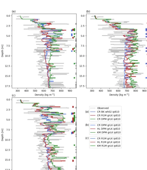
Figure 4.Measured and modelled depth–density profiles at DYE-2 on 11 May 2017. Thick vertical lines show ice layers. The modelled densities are averaged at the vertical resolution of the drilled core. CR: CROCUS, HL: Herron and Langway, KM: Kuipers Munneke.
and so more water tends to be retained and refrozen close to the surface due to stronger capillary forces. Compared to the R1M grLK ip810 experiment, the R1M grA ip810 causes formation of ice layers earlier in the simulation (beginning
in 1996) and shallower in the firn column (Fig. 3e), favour-ing water pondfavour-ing and subsequent runoff (+7 % of the water input over the entirety of the transient model run). Stronger capillarity also means that saturation is higher for percolation to occur, which in turn increases the simulated runoff since more water is in excess of the residual water content. The en-hanced runoff and shallower percolation lead to a higher FAC (+4 %) and a colder 10 m temperature (−0.6 K). In DPM, the flow and refreezing patterns are also altered by the grain-size formulation: DPM grA ip810 produces ice layers much earlier (beginning in summer 1981), at shallower depths and in larger numbers (Fig. 3f). Runoff is however only slightly increased (+2 %). The FAC remains similar to DPM grLK ip810, but the 10 m temperature is 0.3 K lower and the warm bias is thus reduced (an 11 % decrease) (Table 2).
compared to the CROCUS model (−24 %), and, in this case, differences between flow schemes are small with respect to the choice of the densification formulation. Since the warm bias of DPM can cause temperature-dependent densification formulations to overestimate densities, we also compare the three densification formulations coupled to R1M grLK ip810 (Fig. 4c). Similar to the results using the DPM flow scheme, the HL profile agrees reasonably well with the CROCUS model (FAC value is−7 %) but predicts that a metre-thick ice layer formed at 5 m depth (Fig. 4c) during the 2012 summer. Discrepancies between CROCUS and KM are only slightly reduced using R1M; for example, the FAC predicted by KM is 20 % less than that predicted by CROCUS. This can be attributed to greater densities at depth (>8 m) and to much higher densities in the depth range 3–5 m. The latter corre-sponds to the layers affected by meltwater refreezing and considerable latent heat release in the 2012 summer. 4.2 NASA-SE
NASA-SE is a site characterised by high accumulation rates, ranging between 0.5 and 0.8 m w.e. yr−1, and low rates of liq-uid water input, typically between 0.01 and 0.15 m w.e. yr−1 (Fig. 2). Under these conditions, abundant pore space and cold content are available for prompt refreezing of the sum-mer meltwater, so one would expect a smaller sensitivity of the model to the flow scheme applied. In BK, no runoff is produced over the entire simulation (Table 3) since refreez-ing of small amounts of melt does not lead to the formation of impermeable ice layers. R1M and DPM have very low runoff amounts with a small spike in the summer of 2012 when there was 0.38 m w.e. of liquid water input. No ice layer forms in the top 15 m of the firn column using any of the liquid water schemes, in agreement with the observed core (Fig. 5a). Changing the impermeability threshold results in identical model results since no layer exceeds the lowest pos-sible value in the depth range where water percolates. The three water-transport schemes predict a similar FAC; they all underestimate the observed value by approximately 3 % (Ta-ble 3). This is because the mean firn density is well-captured by the model but somewhat overestimated at depths greater than 8 m (Fig. 5a). R1M simulates a single density peak at 8 m depth (Fig. 5a), corresponding to the 2012 summer melt-water percolation, due to capillary forces effectively retain-ing the relatively high meltwater volume produced in that year close to the surface and exposing it to delayed refreez-ing once these layers cool below the freezrefreez-ing point. DPM also produces a density peak (albeit a much smaller one) at a similar depth, and moeffective downward percolation re-sults in a uniform increase in density over the next 3 m. Fi-nally, BK also produces a small density peak; however, this is at a greater depth of 9 m since it assumes water flow to be instantaneous in a time step and the major part of the refreez-ing occurs as water reaches deeper cold layers. Again, none of the percolation schemes capture the observed variability
Figure 5.Measured and modelled depth–density profiles at NASA-SE on 4 May 2016. The modelled densities are averaged at the ver-tical resolution of the drilled core. CR: CROCUS, HL: Herron and Langway, KM: Kuipers Munneke.
in density. Also, despite the low melt/accumulation ratio, the three percolation schemes overestimate the 10 m temperature by 1.4–2.2 K (Table 3).
Increasing the water-holding capacity in BK (BK whCL ip810) leads to a minor increase in the FAC (<1 %) and a 0.9 K cooling of the 10 m temperature, because the sur-face layers have a relatively low density (sursur-face boundary condition of 240 kg m−3 at this site) and thus retain high amounts of water with the whCL parameterisation (Table 3). The R1M and the DPM density profiles are weakly sensitive to a change in the grain-size formulation from grLK to grA (Table 3). This is due to the small meltwater amounts with meltwater refreezing only slightly closer to the surface be-cause of the stronger capillarity retention in the grA models. However, we note that simply changing the grain-size for-mulation in R1M from grLK to grA leads to a 0.4 K colder 10 m temperature and thus decreases the bias with respect to observations by 28 % (Table 3).
Table 3.Model outputs at NASA-SE site. A slash indicates no data.
Refreezing/ Refreezing/ Runoff/ Runoff/ Top 15 m FAC (m) T 10 m (K)
inflow inflow inflow inflow (anomaly vs. (anomaly vs.
(1980–2011) (2012–2015) (1980–2011) (2012–2015) observations) observations, K)
BK (wh02 ip810) 0.97 0.97 0.00 0.00 6.78 (−3 %) 257.91 (+1.94)
R1M (grLK ip810) 0.94 0.89 0.02 0.08 6.78 (−3 %) 257.39 (+1.42)
DPM (grLK ip810) 0.95 0.94 0.01 0.03 6.77 (−3 %) 258.18 (+2.21)
Observations / / / / 6.98 255.97
BK (whCL ip810) 0.95 0.94 0.00 0.02 6.81 (−2 %) 256.97 (+1.00)
R1M (grA ip810) 0.92 0.83 0.04 0.13 6.83 (−2 %) 256.99 (+1.02)
DPM (grA ip810) 0.95 0.92 0.01 0.04 6.78 (−3 %) 258.11 (+2.14)
HL R1M (grLK ip810) 0.93 0.86 0.04 0.11 8.13 (+17 %) 258.19 (+1.22)
KM R1M (grLK ip810) 0.93 0.86 0.03 0.10 7.53 (+8 %) 257.74 (+1.77)
Table 4.Model outputs at KAN-U site. A slash indicates no data.
Refreezing/ Refreezing/ Runoff/ Runoff/ Top 15 m FAC (m) T 10 m (K)
inflow inflow inflow inflow (anomaly vs. (anomaly vs.
(1980–2011) (2012) (1980–2011) (2012) observations) observations, K)
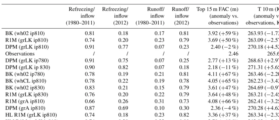
BK (wh02 ip810) 0.81 0.18 0.17 0.81 3.92 (+59 %) 263.93 (−1.73)
R1M (grLK ip810) 0.74 0.20 0.23 0.79 3.69 (+50 %) 263.09 (−2.57)
DPM (grLK ip810) 0.91 0.77 0.07 0.23 2.40 (−2 %) 270.18 (+4.52)
Observations / / / / 2.46 265.66
DPM (grLK ip780) 0.91 0.75 0.07 0.25 2.77 (+13 %) 268.63 (+2.97)
DPM (grLK ip 830) 0.90 0.82 0.07 0.18 2.18 (−11 %) 271.31 (+5.65)
BK (wh02 ip780) 0.78 0.19 0.21 0.81 4.11 (+67 %) 263.46 (−2.20)
BK (whCL ip810) 0.78 0.22 0.19 0.78 4.05 (+65 %) 262.23 (−3.43)
BK (wh02 ip830) 0.83 0.21 0.15 0.79 3.61 (+47 %) 264.69 (−0.97)
R1M (grLK ip830) 0.76 0.20 0.22 0.79 3.64 (+48 %) 263.21 (−2.45)
R1M (grA ip810) 0.66 0.26 0.31 0.73 4.08 (+66 %) 262.41 (−3.25)
DPM (grA ip810) 0.87 0.69 0.10 0.30 2.36 (−4 %) 270.28 (+4.62)
HL R1M (grLK ip810) 0.74 0.18 0.23 0.82 3.36 (+37 %) 263.34 (−2.32)
KM R1M (grLK ip810) 0.74 0.20 0.23 0.80 2.70 (+10 %) 262.82 (−2.84)
4.3 KAN-U
KAN-U is a high-melt site with an average melt rate over the 1980–2013 period of 0.33 m w.e. yr−1, and, in the last 3 years of our simulation (2010–2013), the RCM calculates annual melt exceeding annual accumulation (Fig. 2). Since surface temperatures are relatively high (annual mean around−8◦), refreezing of the summer meltwater depletes the cold content over large depth ranges. Beginning in summer 1990 in the BK simulation, some ice layers are present in the depth range 3–8 m (Fig. 6a), allowing part of the meltwater to run off and impeding percolation to greater depths. At the start of 2012, there is a thick ice layer in the upper 4 m and another one forms at the surface during the summer. As a result, refreez-ing is constrained to the uppermost firn layers and a large part of the water input runs off (Table 4). In R1M, the high water content and the almost-continuous presence of ice layers in the upper 5 m from summer 1986 onwards (Fig. 6b) cause relatively high runoff rates throughout the simulation (28 %
the BK (−39 %) and the R1M (−35 %) simulations, in which runoff limits the amount of meltwater refreezing.
The observations reveal a thick, almost-continuous ice slab over the depth range of 1–7 m (Fig. 8a). Below it, the density is more variable but remains generally high, causing a low FAC (Table 4). Both the BK and the R1M simulation signif-icantly overestimate the FAC (+59 % and+50 %). In con-trast, the average FAC of the DPM simulation is very close to the observed value (−2 %); however, the DPM density profile shows an almost-continuous ice slab from 3 to 17 m depth (Fig. 8a) and does not reproduce the lower-density in-tervals observed. This demonstrates an important limitation of the liquid water schemes: since water cannot be retained in layers exceeding the impermeability threshold, these lay-ers can only further densify by the dry-densification mech-anism and not by water refreezing. The overestimation of the ice slab thickness in the DPM profile is thus compen-sated for by the underestimation of its density, which leads to the good agreement with the observed FAC value. BK repro-duces the presence of the ice slab at 1 m depth, but it underes-timates its thickness and simulated a thick (2 m) low-density region (Fig. 8a). Below the observed ice slab, the agreement with observed average density is reasonable but variability in density is underestimated. Despite also underestimating the thickness of the ice slab, the R1M profile agrees better with the observed density profile: it produces only two thin, low-density layers in the slab and more high-low-density peaks and ice layers below 7 m, which is in better agreement with the observed density variability.
With respect to the 10 m temperature, the BK method is biased cold but gives results in reasonable agreement with the observations (−1.7 K). This bias is more pronounced in R1M (−2.6 K). In contrast, DPM largely overestimates the 10 m temperature (+4.5 K), as a result of its overestimation of percolation and subsequent refreezing at depth.
Changing the impermeability threshold for DPM (DPM wh02 ip780 and ip830) does not alter the pattern of the mod-elled depth–density profile, but the corresponding changes to the density of the ice slab have an impact on the FAC (+15 % for ip780 and −9 % for ip830). Other factors further affect the FAC: runoff rates slightly decrease with higher imper-meability thresholds (Table 4); and the mass of the ice lay-ers increases the overburden stress on the firn column below, increasing the densification rate. In addition, higher (lower) impermeability thresholds lead to warmer (colder) 10 m tem-peratures (+1.1 K for ip830 and−1.6 K for ip780), due to enhanced latent heat release. Compared to BK wh02 ip810, decreasing the impermeability threshold (BK wh02 ip780) leads to the formation of ice layers in earlier years and closer to the surface and thus more runoff (+3 % of the water input over the entirety of the transient model run), which in turn in-creases the FAC (+5 %) and decreases the 10 m temperature (−0.5 K). Increasing the threshold (BK wh02 ip830) has the opposite effect (−8 % for the FAC and+0.8 K for the 10 m temperature compared to BK wh02 ip810). If we instead
al-low for a greater water-holding capacity (BK whCL ip810), the partitioning between runoff and refreezing remains very similar (Table 4). However, the FAC and the 10 m tempera-ture are changed (+3 % and−1.7 K compared to BK wh02 ip810). The lower temperature is due to latent heat release from refreezing being more concentrated in the surface lay-ers (Fig. 6d). The formation of ice laylay-ers earlier in the year and at shallower depths allows part of the underlying firn to remain free of refreezing, which increases the FAC. Fur-thermore, colder temperatures cause a higher firn viscosity, thus decreasing the densification rates. Since the R1M for-mulation both overestimates the FAC and underestimates the 10 m temperature, we test an increase in its impermeability threshold (R1M grLK ip830), allowing for deeper percola-tion. Both the decrease in FAC (−1 %) and increase in 10 m temperature (+0.1 K) compared to R1M grLK ip810 are mi-nor.
With the grA formulation in DPM (DPM grA ip810), wa-ter is more efficiently transferred vertically through the pref-erential flow domain, which causes an increase in the num-ber of ice layers formed during the simulation (Fig. 6f), a slight decrease in FAC (−2 %) and a slight increase in the 10 m temperature (+0.1 K) relative to DPM grLK ip810. The nearly continuous ice slab, which extends to 17 m depth be-low the final winter accumulation, explains the weak sensi-tivity of the final FAC and 10 m temperature values of DPM to grain size. In contrast, applying the grA formulation in R1M (R1M grA ip810) leads to a considerable increase in FAC (+11 %) and a decrease in 10 m temperature (−0.7 K) compared to R1M grLK ip810. This is due to higher wa-ter content during percolation events and, especially in the most recent years of our simulation, refreezing and ice-layer formation at shallower depths (Fig. 6e). This increases the runoff and isolates the deeper firn from meltwater percola-tion. As in the cases of DYE-2 and NASA-SE, the change in FAC due to different grain-size formulations in R1M is greater than the change due to switching from BK to R1M (Table 4).
Figure 6.Modelled firn density at KAN-U.(a)BK wh02 ip810,(b)R1M grLK ip810,(c)DPM grLK ip810,(d)BK whCL ip810,(e)R1M grA ip810, and(f)DPM grA ip810; black indicates ice layers.
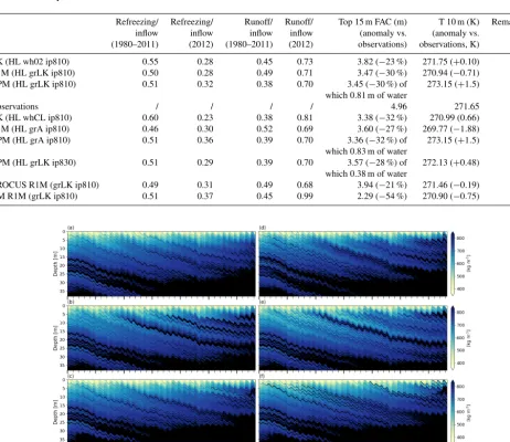
Figure 7.Volumetric water content at the KAN-U site for DPM grLK ip810 in(a)matrix flow domain and(b)preferential flow domain; note the difference in scales.
Figure 8.Measured and modelled depth–density profiles at KAN-U on 28 April 2013. Thick vertical lines show ice layers. The modelled densities are averaged at the vertical resolution of the drilled core. CR: CROCUS, HL: Herron and Langway, KM: Kuipers Munneke.
of the densification formulation has a greater influence on the model than the choice of liquid water scheme and of any of their respective parameterisations presented here, in spite of the high water input at this site.
4.4 FA13
The FA13 site is representative of conditions in the southeast part of the GrIS; it has both high accumulation and high melt rates (mean 1980–2012 rates of 1.09 and 0.64 m w.e. yr−1 re-spectively, Fig. 2). This favours the insulation of summer per-colating meltwater from winter atmospheric temperatures, typically leading to the formation of PFAs (Kuipers Munneke et al., 2014). Here, the initial conditions and the spin-up pro-cess cause the deep firn to be close to the melting point at the start of the transient run.
observed core shows that the 810 kg m−3density is reached and maintained from 24 m depth. The CROCUS densifi-cation scheme predicts that this density horizon occurs at 60 m depth. Since CROCUS has been developed for seasonal snow, the densification at high overburden stress is proba-bly not well-captured by the model (Stevens, 2018). Because of this, we base our simulations for FA13 on the HL den-sification model, which predicts this transition depth to be around 21 m.
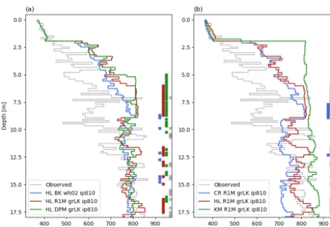
The total refreezing rates are similar for the three flow schemes (Table 5). Since the deep firn is close to the melt-ing point, the total refreezmelt-ing amounts are essentially deter-mined by the cold content provided in winter, and the precise behaviour of the percolation has a minor impact. However, variability of refreezing with depth differs between schemes, which leads to differences in the 15 m FAC values (Table 5) and in the modelled depth–density profiles (Figs. 9a, b, and c and 10a). FAC is consistently underestimated (−23 to −30 %) because firn density is overestimated above 10 m. R1M and DPM overestimate density most strongly with FAC values 9 % and 10 % smaller than BK respectively, and both schemes simulate the presence of a thick ice layer in the up-per 10 m of the firn, which is not observed in the core. The BK model produces only a single thin ice layer in the upper 10 m (0.2 m thick at 9 m depth), which is in good agreement with the observations (showing a single thin ice layer at 7.5 m depth). Below 10 m, the modelled densities are generally in better agreement and all the schemes produce several ice lay-ers (Figs. 10a and 9a, b and c).
In the absence of any shallow ice layer throughout most of the simulation (Fig. 9a, b and c), meltwater is free to perco-late through the winter accumulation layers and to deplete their cold content. The flow schemes have different abili-ties to store liquid water, which leads to small variations in runoff and refreezing rates. In BK, water is retained accord-ing to the water-holdaccord-ing capacity (Fig. 11a) and refreezes during subsequent winters. In contrast, DPM allows perco-lation down to the firn–ice-sheet transition where it ponds to form an aquifer (Fig. 11d and e). This leads to a signif-icant reduction of runoff amounts during the aquifer build-up (−6 % of the water input over the entirety of the tran-sient model run compared to BK), and the water remaining in the firn column is essentially constrained by the maximal amount of water we allow in the aquifer (1.65 m). In theory, the same mechanism could be simulated by R1M, but the percolating water is depleted before it reaches the bottom of the firn column (Fig. 11b). This is due to refreezing, to the lateral runoff parameterisation and to the presence of ice lay-ers in the upper 10 m. No water play-ersists through the winter seasons, which illustrates the model artefact that the effective saturation must be strictly positive for the stability of the RE (Sect. 3.2). Thus, the refreezing rates are slightly lower than in BK since no residual water is stored and later exposed to winter refreezing (Table 5).
The build-up of the aquifer starts very early (in the sum-mer of 1981) when DPM is turned on in the transient run due to the low refreezing capacity of the deep firn. The depth of this aquifer is constrained by the impermeability thresh-old applied, which determines where the model places the firn–ice transition. This depth is at 33 m in 1981 and 21 m in 2013, with the decrease being caused by enhanced densifica-tion. The aquifer is fed only by preferential flow (Fig. 11e) since matrix flow cannot reach the water table due to runoff, refreezing and the presence of ice layers in the firn column.
From 1994 and onwards the total simulated water content in summer is only regulated by the maximum allowed in the model (1.65 m). Since the water table is at a shallow depth towards the end of the simulation (7.5 m), the propagation from the surface of the cold winter temperatures can refreeze part of the saturated layers. This leads to the formation and progressive thickening of the shallow, thick ice layer. Also, the shallowness of the aquifer causes 23 % of the porosity in the top 15 m to be filled with liquid water and the 10 m temperature to be at the melting point.
The higher impermeability threshold in DPM grLK ip830 increases the depth of the calculated firn–ice transition, pro-ducing a deeper aquifer that extends between 12 and 29 m depth at the end of the simulation, similar to the 12–37 m depth range observed by Koenig et al. (2014). Compared to DPM grLK ip810, the increased depth leads to less refreez-ing in the shallowest layers of the aquifer and thus a higher FAC value (+3 %) and a 10 m temperature below the melt-ing point.
The grain-size formulation following Arthern et al. (2010) (DPM grA ip810) reduces the ability of preferential flow to transport water down to the firn–ice transition but instead favours formation of discrete ice layers in the firn column (Fig. 9f). In this case the aquifer does not start to form until summer 1988, but the final aquifer structure (also between 7.5 and 21 m), the FAC value (−3 % for grA), and the par-titioning between refreezing and runoff are similar to those simulated using grLK (Table 5). In R1M, the sensitivity to grain size is noticeable in the firn-structure evolution with differences in ice-layer formation between R1M grLK ip810 and R1M grA ip810 (Fig. 9b and e). The final FAC value (+4 % for grA) and the meltwater partitioning remain sim-ilar (Table 5) between R1M grLK and R1M grA, as for the case of DPM grLK and DPM grA. This can be explained by the total refreezing’s stronger dependence on the firn thermal structure than on the percolation pattern at this site.
Table 5.Model outputs at FA13 site. A slash indicates no data.
Refreezing/ Refreezing/ Runoff/ Runoff/ Top 15 m FAC (m) T 10 m (K) Remaining inflow inflow inflow inflow (anomaly vs. (anomaly vs. water (1980–2011) (2012) (1980–2011) (2012) observations) observations, K) (m) BK (HL wh02 ip810) 0.55 0.28 0.45 0.73 3.82 (−23 %) 271.75 (+0.10) 0 R1M (HL grLK ip810) 0.50 0.28 0.49 0.71 3.47 (−30 %) 270.94 (−0.71) 0 DPM (HL grLK ip810) 0.51 0.32 0.38 0.70 3.45 (−30 %) of 273.15 (+1.5) 1.53
which 0.81 m of water
Observations / / / / 4.96 271.65 1.65 BK (HL whCL ip810) 0.60 0.23 0.38 0.81 3.38 (−32 %) 270.99 (0.66) 0.09 R1M (HL grA ip810) 0.46 0.30 0.52 0.69 3.60 (−27 %) 269.77 (−1.88) 0 DPM (HL grA ip810) 0.51 0.36 0.39 0.70 3.36 (−32 %) of 273.15 (+1.5) 1.48
which 0.83 m of water
DPM (HL grLK ip830) 0.51 0.29 0.39 0.70 3.57 (−28 %) of 272.13 (+0.48) 1.64 which 0.38 m of water
CROCUS R1M (grLK ip810) 0.49 0.31 0.49 0.68 3.94 (−21 %) 271.46 (−0.19) 0 KM R1M (grLK ip810) 0.51 0.37 0.45 0.99 2.29 (−54 %) 270.90 (−0.75) 0
Figure 9.Firn density at FA13.(a)BK wh02 ip810,(b)R1M grLK ip810,(c)DPM grLK ip810,(d)BK whCL ip810,(e)R1M grA ip810, and(f)DPM grA ip810; black indicates solid ice.
is stored in the saturated layers of the aquifer simulated in DPM.
We compare the three different densification models (CROCUS, HL, KM) using the R1M grLK ip810 flow scheme and these show important differences in the final modelled depth–density profiles (Fig. 10b). CROCUS agrees reasonably well with HL in the top 6 m, but, as mentioned above, it has a strong low-density bias at greater depths. Since CROCUS simulates lower densification rates, its un-derestimation of the FAC value in the upper 15 m (−21 %) is smaller than in HL (−30 %), but it is clearly not representa-tive of the density conditions below 15 m. KM predicts a firn column below the last winter’s accumulation entirely at the ice density. The model thus identifies a firn–ice-sheet tran-sition at shallow depth (∼2 m), which the water can reach before being depleted by the lateral runoff parameterisation
Figure 10.Measured and modelled depth–density profiles at FA13 on 10 April 2013. Thick vertical lines show ice layers. The modelled densities are averaged at the vertical resolution of the drilled core. CR: CROCUS, HL: Herron and Langway, KM: Kuipers Munneke.
5 Discussion
The three liquid water schemes show consistent behaviour between sites. R1M generally predicts slower downward per-colation of water than the other schemes, which leads to more near-surface refreezing, the formation of near-surface ice layers, more lateral runoff, and thus lower densities and lower temperatures in deeper firn. As a result, when com-pared to observations R1M tends to reach higher FAC values and to underestimate 10 m temperatures. The BK formula-tion with the Coléou and Lesaffre (1998) parameterisaformula-tion for the water-holding capacity leads to the same effects, but they are amplified. The underestimation of the 10 m tempera-ture is stronger, suggesting that BK whCL does not allow for deep enough percolation. BK with the lower water-holding capacity (BK wh02) leads to a partitioning of the water input between refreezing and runoff similar to the more complex R1M at the four sites. As a result, the FAC values predicted by BK wh02 and R1M generally agree (maximum difference less than 10 %), as do the temperatures at 10 m depth (max-imum difference less than 1 K). The FAC values and 10 m temperatures of R1M at the end of the model runs always lie in the range of the ones obtained with different parame-terisations of BK. This suggests that BK can produce results similar to R1M, provided it is parameterised appropriately.
DPM exhibits a different behaviour: it effectively brings water to greater depths, depleting the deep-firn pore space and cold content. Even in the presence of shallow ice lay-ers hindering matrix flow, the preferential flow implementa-tion still ensures efficient vertical water transport, and runoff amounts remain low. This suggests that transfer mechanisms to the preferential flow domain implemented in DPM are more effective in draining ponding water than the lateral runoff parameterisation. Due to large FAC underestimation and 10 m temperature overestimation, the data–model
mis-match of DPM with respect to these variables is signifi-cantly greater than that of R1M and BK. DPM is better at producing density variability in depth, which is underesti-mated in all schemes at all sites. Also, in contrast to the two other schemes, DPM can form ice layers even in summers of average melt, and it is able to simulate the persistence of deep saturated firn layers at the FA13 site. In this respect our findings support those of Wever et al. (2016), who high-light the tendency of DPM to produce ice layers at various depths in alpine snowpack simulations and thus to reproduce depth–density variability. It is important to bear in mind that we only use the dual-permeability water scheme of SNOW-PACK in DPM and not the other physics of this model; the re-sults produced by the full SNOWPACK model would be dif-ferent because it has its own formulations for snow mechan-ical and thermal properties. In particular, DPM relies heav-ily on the grain size, and it would thus benefit from better representations of the firn’s structural properties. Moreover, the primary purpose of the DPM implementation in SNOW-PACK is to reproduce the occurrence of ice layers in a sea-sonal alpine snowpack (Wever et al., 2016), whereas in this study we evaluate its ability to simulate representative firn depth–density profiles over the course of numerous decades. BK with low water-holding capacity is usually used to mimic preferential flow (Reijmer et al., 2012). However, our findings suggest that, in fact, this more closely represents ma-trix flow as modelled using the Richards equation. We sug-gest that, in order to use BK in this way, percolation of some meltwater in the presence of ice layers should be considered. The lack of variability in density in the modelled profiles cannot only be attributed to inaccuracies in the percolation– refreezing process. This is demonstrated in the example of NASA-SE: the layers of the density peak observed around 1 m depth (Fig. 4a and b) were deposited during the final win-ter of the simulation (2015–2016). As such, these have only been influenced by the percolation and refreezing of negligi-ble amounts of liquid water. The consistent underestimation of density variability across all schemes indicates that one or several other factors that are not or poorly represented by firn models likely play a crucial role in firn evolution. These factors may include horizontal water flow, prolonged pond-ing of water in soaked firn close to the surface, variability in fresh snow density, the effects of firn microstructure and im-purity content on densification, wind packing and short-term weather fluctuations. Moreover, the validity of the firn model relies on the accuracy of the climatic forcing.