https://doi.org/10.5194/tc-12-2741-2018
© Author(s) 2018. This work is distributed under the Creative Commons Attribution 4.0 License.
West Antarctic sites for subglacial drilling to test for
past ice-sheet collapse
Perry Spector1,2, John Stone1, David Pollard3, Trevor Hillebrand1, Cameron Lewis4, and Joel Gombiner1
1Department of Earth and Space Sciences, University of Washington, Seattle, WA, USA 2Berkeley Geochronology Center, 2455 Ridge Road, Berkeley, CA, USA
3Earth and Environmental Systems Institute, Pennsylvania State University, University Park, PA, USA 4Center for Remote Sensing of Ice Sheets (CReSIS), University of Kansas, Lawrence, KS, USA
Correspondence:Perry Spector (spectorp@gmail.com) Received: 30 April 2018 – Discussion started: 4 June 2018
Revised: 31 July 2018 – Accepted: 8 August 2018 – Published: 24 August 2018
Abstract. Mass loss from the West Antarctic Ice Sheet (WAIS) is increasing, and there is concern that an incip-ient large-scale deglaciation of the marine basins may al-ready be underway. Measurements of cosmogenic nuclides in subglacial bedrock surfaces have the potential to estab-lish whether and when the marine-based portions of the WAIS deglaciated in the past. However, because most of the bedrock revealed by ice-sheet collapse would remain below sea level, shielded from the cosmic-ray flux, drill sites for subglacial sampling must be located in areas where thinning of the residual ice sheet would expose presently subglacial bedrock surfaces. In this paper we discuss the criteria and considerations for choosing drill sites where subglacial sam-ples will provide maximum information about WAIS extent during past interglacial periods. We evaluate candidate sites in West Antarctica and find that sites located adjacent to the large marine basins of West Antarctica will be most diagnos-tic of past ice-sheet collapse. There are important consider-ations for drill site selection on the kilometer scale that can only be assessed by field reconnaissance. As a case study of these considerations, we describe reconnaissance at sites in West Antarctica, focusing on the Pirrit Hills, where in the summer of 2016–2017 an 8 m bedrock core was retrieved from below 150 m of ice.
1 Introduction
There is strong but indirect evidence for a diminished West Antarctic Ice Sheet (WAIS) during some past warm inter-glacial periods of the Pleistocene. Coastal records of for-mer sea-level highstands (see reviews in Dutton et al., 2015), along with geological evidence from Antarctica (Scherer et al., 1998), ice-sheet modeling experiments (e.g., Pollard and DeConto, 2009), and other lines of evidence (e.g., Barnes and Hillenbrand, 2010; NEEM community members, 2013; see review in Alley et al., 2015) suggest large-scale deglacia-tion of the WAIS within the past ∼1 million years (Myr), which may have occurred as recently as the last interglacial period,∼125 thousand years before present (kyr BP). It has also been suggested that the WAIS, along with the Green-land Ice Sheet and parts of the East Antarctic Ice Sheet, disappeared during the mid-Pliocene (∼3 Myr BP), the last time atmospheric CO2concentrations reached modern levels.
However, the evidence for this, which largely consists of rel-ative sea-level data and marine oxygen isotope records, has large uncertainties, which preclude robust estimates of sea-level and ice-sheet volume during this period (see reviews in Dutton et al., 2015 and Raymo et al., 2017).
modeling suggests that an incipient collapse of the ice sheet is underway in this sector (e.g., Joughin et al., 2014). How much and how quickly future sea level will rise due to WAIS deglaciation remains unknown (Scambos et al., 2017), but continued ice loss could eventually increase global mean sea level by 3–4 m (Bamber et al., 2009). Knowledge of ice-sheet extent during interglacials warmer and more prolonged than the Holocene would be invaluable for understanding, and po-tentially predicting, the future stability or instability of the WAIS. Geological observations from West Antarctica which constrain the configuration of the WAIS during former inter-glacial periods remain scarce because evidence of its limits during these times is concealed beneath the present-day ice sheet.
One potential source of evidence is the presence or absence of long-lived cosmogenic nuclides in subglacial bedrock. Because most cosmic radiation is absorbed by as lit-tle as 5–10 m of ice cover, discovering significant concentra-tions of these nuclides would provide unambiguous evidence for former ice-free conditions and could establish whether the WAIS collapsed during the past few million years. At sites affected by a single collapse, cosmogenic-nuclide mea-surements can directly date that event. In the case of more complex deglaciation histories, the same data record the cu-mulative exposure time of the bedrock surface. Although cosmogenic nuclides have the potential to unambiguously in-dicate past ice-sheet collapse on timescales ranging from the Holocene to the Pliocene, the power of the method depends on careful site selection. In this paper we describe the crite-ria and considerations for choosing subglacial sampling sites where cosmogenic-nuclide data will provide the maximum amount of information about WAIS extent during past inter-glacials.
In central Greenland, a bedrock core was opportunistically retrieved from below the full thickness of the ice sheet at the GISP2 drilling site. Concentrations of cosmogenic10Be and
26Al in the core require periods of prolonged exposure during
the Pleistocene when the ice sheet was largely absent (Schae-fer et al., 2016; Nishiizumi et al., 1996). In contrast to this work, bedrock recovered from below the thick portions of the WAIS would not be capable of providing equivalent informa-tion because the bed in these areas is located far below sea level (Fig. 1) and would remain submerged, shielded from the cosmic-ray flux, if the ice sheet collapsed. Establishing whether the thick, marine-based portions of the WAIS disap-peared in the past will therefore require drilling through ad-jacent, thinner portions of the ice sheet into subglacial high-lands that would be exposed by ice thinning during collapse events.
In the 2016–2017 austral summer, the first cores of sub-glacial bedrock from West Antarctica were recovered from the Pirrit Hills and the Ohio Range (Fig. 1), which was made possible by recent advances in sub-ice drilling technology (e.g., Goodge and Severinghaus, 2016). For these as well as future drilling efforts to provide meaningful information
about past WAIS configurations, the measurements made on the recovered bedrock must be representative of the past ice thickness at the drill site, which in turn must be linked to the extent of the broader ice sheet. In Sect. 2 of this paper, we de-scribe cosmogenic-nuclide considerations that guide drill site selection. In Sect. 3, we use an ice-sheet model to predict the areas of the WAIS where significant thinning (and thus ex-posure of presently subglacial bedrock) would occur during collapse events. In Sect. 4, we evaluate a group of candidate drill sites throughout West Antarctica. Finally, in Sect. 5, we describe reconnaissance work at three sites in West Antarc-tica, with emphasis on the Pirrit Hills, which we present as a case study of drill site selection on the scale of an individual nunatak.
2 Cosmogenic nuclide considerations for drill site selection
2.1 Strategies for subglacial bedrock sampling and analysis
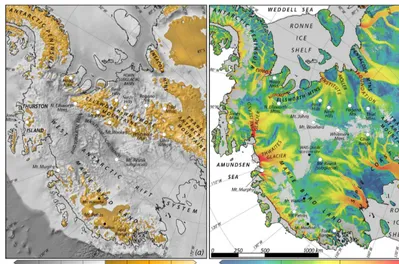
Figure 1.Maps of West Antarctica. The left map is colored to identify areas where the bed is presently below sea level and areas where it is above (Fretwell et al., 2013). The right map is colored to show the velocity of grounded ice (Rignot et al., 2011). White circles show the locations of possible drill sites discussed in the text. Black circles show the locations of other sites discussed in the text.
2.2 Subglacial bedrock lithology
The central portion of West Antarctica is composed of three tectonic and topographic blocks, the Ellsworth–Whitmore Mountains, Marie Byrd Land, and what is known as the Thurston Island region, which are separated by low-lying ar-eas of the West Antarctic Rift System (Fig. 1). The portions of the bed that would be above sea level if the WAIS col-lapsed (accounting for isostatic effects) are primarily located in these three tectonic regions; however there are isolated peaks and plateaus, such as subglacial Mt. Resnik (Behrendt et al., 2007), which rise above sea level from the deep marine basins (Fig. 1).
Drilling into these subglacial highlands must target rock types in which useful cosmogenic nuclides can be mea-sured. Commonly measured nuclides (and their half-lives) include 10Be (1.4 Myr),26Al (0.7 Myr),21Ne (stable), 36Cl (0.3 Myr),3He (stable), and14C (5.7 kyr). If more of these nuclides can be measured, more restrictive time constraints can be placed on exposure episodes that may have occurred in the distant and/or recent past. Because (i) all of these nu-clides (except36Cl) can be measured in quartz, and (ii) their production rates are best known for quartz, quartz-rich rocks would allow the glacial history to be constrained over a large range of timescales. Igneous or metamorphic rocks of granitic composition would permit the greatest variety of analyses because, in addition to containing quartz, they also
contain potassium feldspar and (commonly) Cl-rich mica in which 36Cl can be measured. Other analytical strategies could be applied to the volcanic rocks that underlie large ar-eas of the WAIS. For example, cosmogenic3He,21Ne, and
36Cl could be measured in basaltic pyroxene, or in a
com-bination of quartz and sanidine from more felsic volcanic rocks. However, the relative abundance of useful minerals such as these is also important because of the small amount of rock that can be retrieved by subglacial drilling (Goodge and Severinghaus, 2016).
(iii) along sections of the Marie Byrd Land coast. In addition to granitic sites, in Fig. 1 we also include quartzite peaks of the northern Ellsworth Mountains, the isolated quartzite nunatak of Mt. Johns, and subglacial Mt. Resnik, which, al-though likely volcanic (Behrendt et al., 2007), is a tempting drill target because (i) it lies upstream of where Scherer et al. (1998) found evidence for a large-scale Pleistocene deglacia-tion of the WAIS, (ii) its conical form and high relief sug-gest that it erupted subaerially when the ice sheet was absent (Behrendt et al., 2007), and (iii) its summit is only∼330 m below the ice surface (Morse et al., 2002).
2.3 Preservation of the cosmogenic-nuclide record Because the cosmogenic-nuclide record is primarily pro-duced in the topmost few meters of an exposed bedrock sur-face, its survival requires that the bedrock remains continu-ously protected from erosion. This is most likely to be the case in areas that are surrounded by slow-flowing ice and where thickening of the ice sheet during past glacial peri-ods such as the Last Glacial Maximum (LGM) was minimal. Other factors which promote cold-based ice are high accu-mulation rates, low surface temperatures, and a low geother-mal heat flux. As discussed in Sect. 4, sites in the WAIS inte-rior are likely to have preserved subglacial bedrock surfaces hundreds of meters below the modern ice level. Preserved subglacial surfaces also likely exist near the ice-sheet mar-gin; however, it may be more difficult to identify these sites with confidence. Although subglacial bedrock samples that have remained continuously uneroded will provide the great-est constraints on the glacial history, samples that have expe-rienced low rates of erosion may also be of use, provided that the erosion history can be estimated. As mentioned above, this can be accomplished by measuring cosmogenic nuclides not only in the subglacial bedrock surface but also in depth profiles along the length of short (∼3–6 m) bedrock cores (Ploskey and Stone, 2012).
A related concern to bedrock erosion is the possibility that presently subglacial surfaces remained concealed by till, soil, or snow when the ice sheet disappeared in the past. Failure to account for past surface cover would cause the true expo-sure history to be underestimated. Analysis of the subglacial bedrock core from the GISP2 site in central Greenland sug-gests that the present-day bedrock surface was covered by a thin layer of material when the ice sheet disappeared dur-ing the Pleistocene (Schaefer et al., 2016). Soil accumula-tion there is plausible because debris-rich basal ice in the GISP2 and other Greenland ice cores contains evidence for a vegetated landscape during one or more interglacial periods in the past million years (Souchez et al., 2006; Willerslev et al., 2007; Bierman et al., 2014). In Antarctica, however, fossil organisms and pollen from sites spanning the conti-nent show that a tundra landscape went extinct around the mid-Miocene, and that the climate has been continuously po-lar since that time (Lewis et al., 2008; Anderson et al., 2011;
Wei et al., 2014; Ashworth and Erwin, 2016). Although soil is unlikely to have covered drill targets in Antarctica during former interglacial periods, accumulated till is possible. In the vicinity of outcropping mountains where drill sites will probably be located, englacial debris commonly accumulates in blue-ice areas, and subsequent thinning could drape the underlying bedrock with a layer of till. As discussed below in Sect. 5, this concern can be mitigated by locating drill sites above subglacial ridges where the likelihood of till or snow cover is minimal.
3 Where will WAIS collapse cause the largest changes? WAIS collapse is theorized to occur via a feedback in which initial retreat of the grounding line into deeper water causes more ice to flow across the grounding line (Weertman, 1974; Schoof, 2007). This accelerates the flow of the ice sheet up-stream, causing it to thin, which in turn causes previously grounded ice to float as the grounding line recedes farther inland. The thinning of upstream grounded ice is impor-tant because it is the link between withdrawal of ice from the marine basins and the exposure of presently subglacial bedrock surfaces in the WAIS interior. Therefore, an over-arching criterion is that drill sites be located in areas that experience the largest change in ice thickness during col-lapse events, bearing in mind the need to avoid sites where ice flow may have been erosive in the past. Recent observa-tions in the Amundsen Sea sector show that thinning induced by grounding-line retreat is greatest near the ice-sheet mar-gin, but remains detectable hundreds of kilometers upstream (Pritchard et al., 2012). This suggests that although large por-tions of the WAIS are prone to thinning during deglaciapor-tions, some sites will be more or less diagnostic of past ice-sheet collapse.
if the WAIS collapsed during past interglacial periods, the greatest thinning likely occurred at sites directly adjacent to the deep marine basins in West Antarctica that became ice free, such as Bentley Subglacial Trench (Fig. 1).
In order to examine the transient response of different parts of the WAIS to collapse events, and thereby identify which areas will be most diagnostic of past deglaciations, we use the Penn State University ice-sheet model (PSU-3D) to simu-late the Antarctic Ice Sheet continuously over the past 5 Myr. This time period, from the early Pliocene to the present, covers a large range of glacial–interglacial climates and is comparable to the time period that can be investigated with cosmogenic-nuclide measurements. In comparison, most ex-isting collapse simulations depict only a single deglaciation (e.g., Feldmann and Levermann, 2015) or are equilibrium models (e.g., de Boer et al., 2015), which may not represent ice-sheet behavior during short-lived events such as Pleis-tocene interglacial periods.
The model we use solves a hybrid combination of the scaled dynamical equations for the flow of grounded and floating ice (Pollard and DeConto, 2009, 2012a, b). It is sim-ilar to that presented in Pollard and DeConto (2009); how-ever it uses basal sliding coefficients derived from inverse calculations, as well as improved parameterizations of ice-shelf calving and sub-ice oceanic melting (Pollard and De-Conto, 2012b). A parameterization by Schoof (2007) allows for reasonably accurate simulations of grounding-line migra-tion on the coarse grids that are required for multimillion year model runs. We use a 40 km horizontal grid, which, although coarse, is comparable to the resolution with which the bed is known in the vicinity of many of the candidate drill sites (Fretwell et al., 2013). Bedrock deformation in the model is treated as an elastic lithosphere above a viscous astheno-sphere that relaxes toward isostatic equilibrium. The model includes two processes that exacerbate retreat during warm climates: (i) hydrofracture of ice shelves due to surface wa-ter draining into crevasses and (ii) structural failure of ice cliffs at the grounding line (Pollard et al., 2015).
The model is forced with parameterizations of surface temperature, precipitation, sub-ice-shelf melting, and sea level, which have been described in previous publications (Pollard and DeConto, 2009, 2012a). These parameteriza-tions are largely funcparameteriza-tions of a stacked benthicδ18O record (Lisiecki and Raymo, 2005) and orbital insolation variations (Laskar et al., 2004). In this run, we add the influence of long-term atmospheric CO2decline by prescribing a linear ramp
from 400 to 280 ppmv CO2between 3 and 2 Ma, with
cor-responding small uniform shifts to atmospheric and oceanic temperatures. This results in generally smaller model ice volumes prior to 3 Myr compared to Pollard and DeConto (2009). The parameters for the simulation shown in Fig. 2 have been calibrated in previous model experiments (e.g., Pollard and DeConto, 2012a, b; Pollard et al., 2016). Be-cause many of the parameters related to the climate forcing and aspects of the model physics are uncertain, and
alterna-tive values can affect the size of the ice sheet and its rate of change, we use this simulation as a guide to how ice thick-ness at candidate drill sites responds to deglaciation of the marine basins rather than an accurate depiction of the ice sheet through time.
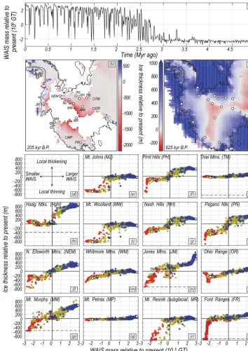
The model is sampled every 5000 years, which sufficiently captures the ice sheet’s variations and results in minimal aliasing. The modeled ice sheet transitions rapidly between expanded and contracted configurations on orbital frequen-cies that reflect the climate forcing (Fig. 2). The simulated ice sheet was smaller than present prior to ∼2.7 Myr BP, at which time its average size began to increase, and col-lapsed configurations with little or no marine-based ice in West Antarctica became less frequent. Some warm periods of the Pleistocene resulted in full deglaciation of the marine basins, leaving small ice sheets on areas of high topography, as shown in Fig. 2b. During other interglacial periods, thin-ning and grounding-line retreat were more limited and sea-ways were unable to link the Amundsen, Ross, and Weddell seas. Although accumulation rates increase over the resid-ual ice sheet during deglaciations, in most areas this is in-sufficient to offset the dynamic thinning. Thinning is typi-cally greatest directly upstream of the retreating grounding line, especially in areas adjoining deep marine basins that be-come ice free, as expected from the considerations described above.
In most areas of central West Antarctica, the mod-eled present-day ice thickness closely matches observations (Fig. 3). The one important exception is in the Weddell Sea sector, where the grounding line in the model is located in-land of Robin Subglacial Basin (compare to Fig. 1). Because ice thickness in Fig. 2e–s is shown relative to the modeled present-day ice sheet, this misfit causes thinning during in-terglacial periods to be underestimated and thickening dur-ing glacial periods to be overestimated at sites upstream of this area. The magnitude of this effect is difficult to quantify due to the transient nature of the model, but at sites directly upstream (e.g., Pirrit Hills, Nash Hills, and Pagano Nunatak) it will likely exceed 100 m. For individual sites in Fig. 2e–s, this would have the effect of shifting points uniformly along theY axis, but not changing their position relative to each other.
4 Evaluation of candidate drill sites
0 0.5 1 1.5 2 2.5 3 3.5 4 4.5 5 -2
0 2
WAIS mass relative to present (10 6 GT)
Time (Myr ago)
Pliocene (5.0–2.58 Myr B.P.) Early Pleistocene (2.58–0.8 Myr B.P.) Late Pleistocene (0.8–present Myr B.P.) -800
-600 -400 -2000 200 400 600 800
-800 -600 -400 -2000 200 400 600 800
Ice thickness relative to present (m) -800-600 -400 -2000 200 400 600 800
-3 -2 -1 0 1 2 3 -3 -2 -1 0 1 2 3 -3 -2 -1 0 1 2 3 -3 -2 -1 0 1 2 3 -800
-600 -400 -2000 200 400 600 800
WAIS mass relative to present (106 GT)
Mt. Johns (MJ) Pirrit Hills (PH) Thiel Mtns. (TM)
Haag Ntks. (HgN) Mt. Woollard (MW) Nash Hills (NH) Pagano Ntk. (PN)
N. Ellsworth Mtns. (NEM) Whitmore Mtns. (WM) Jones Mtns. (JM) Ohio Range (OR)
Mt. Murphy (MM) Mt. Petras (MP) Mt. Resnik (subglacial; MR) Ford Ranges (FR) Local thickening
Local thinning Larger WAIS Smaller
WAIS
(l)
(a)
(d) (e) (f) (g)
(h) (i) (j) (k)
(m) (n) (o)
(p) (q) (r) (s)
205 kyr B.P. 625 kyr B.P.
PH TM HgN
MW NH PN NEM
MJ WM JM
OR
MM
MP MR
FR
Ice thickness relative to present (m)
-2000 -1500 -1000 -500 0 500
-200 0 200 400 600 800 1000
(b) (c)
-1500 -1000 -500 0 500 1000 1500 Modeled modern ice thickness minus
BEDMAP2 ice thickness (m)
Figure 3.The difference between the modeled modern thickness of grounded ice and the thickness of grounded ice in Bedmap2 (Fretwell et al., 2013). The grounding line for the modeled ice sheet is inland of Robin Subglacial Basin.
4.1 Sensitivity of sites to deglaciation of different parts of the WAIS
During collapse episodes simulated by the ice-sheet model, the grounding line retreats rapidly over deep marine basins and is ultimately halted once it reaches shallow water. Be-cause further retreat can only occur slowly and in the pres-ence of a warm atmosphere, the ice-sheet margin is com-monly pinned to a narrow band that closely follows the perimeter of the highland regions (Figs. 1 and 2). This is not unique to our simulation; rather it is a robust feature of ice-sheet models forced with interglacial climates (e.g., Bamber et al., 2009; de Boer et al., 2015; Feldmann and Levermann, 2015; DeConto and Pollard, 2016; Golledge et al., 2017). The model demonstrates that in areas that remain glaciated, thinning occurs as the grounding line approaches, but then stops once the grounding line stabilizes, even if deglaciation continues in other sectors of the WAIS. The implication of this is that the magnitude of thinning at candidate drill sites is most directly controlled by the proximity of the ground-ing line and the thickness of ice lost from the marine basins immediately downstream and less by ice-sheet changes else-where in West Antarctica.
At sites not adjoined to large marine basins, such as the Ford Ranges and the Jones Mountains, it may be difficult to know whether subglacial evidence of past exposure resulted from large-scale WAIS deglaciation or from modest retreat of the ice-sheet margin locally. In a related way, ice thinning at the Pirrit Hills, Nash Hills, and Pagano Nunatak is likely to be controlled most strongly by deglaciation of Robin Sub-glacial Basin, which underlies the Institute and Möller ice
streams (Fig. 1). Therefore, these sites may not be as sensi-tive to the presence or absence of grounded ice in the much larger basins of the Amundsen Sea and Ross Sea sectors of the WAIS. A potential caveat to this is that our simulation, as well as others using the PSU-3D ice-sheet model (e.g., De-Conto and Pollard, 2016), shows that the large marine basins deglaciate in unison, implying that evidence for deglaciation from one sector could be extrapolated to other areas in West Antarctica. At sites on the periphery of the large basins in the Ross and Amundsen sectors (i.e., Mt. Murphy, Mt. Resnik, the Ohio Range, the Whitmore Mountains, Mt. Woollard, Mt. Johns, and the northern Ellsworth Mountains), ice levels will likely be diagnostic of whether full collapse of the WAIS has occurred in the past.
4.2 Magnitude, timing, and frequency of thinning The areas where the model predicts large drawdowns, not only during the most severe interglacial periods (which occur during the Pliocene in the simulation) but also during briefer warm periods of the Pleistocene, are the most likely areas to find evidence of past deglaciation in the form of previously exposed subglacial bedrock. The two sites that exhibit the greatest and most consistent ice loss are Mt. Woollard and Mt. Johns, which thin by up to∼800 m during the Pliocene, the Early Pleistocene, and the Late Pleistocene (Fig. 2e, i). The frequency of deglaciation at these sites is perhaps not surprising as they are located at the head of the Thwaites Glacier catchment, where (i) there is concern at present about the stability of the grounding line (e.g., Scambos et al., 2017), and (ii) there are no major topographic obstacles to impede the grounding line until it reaches the Ellsworth– Whitmore Mountains. The large magnitude of deglaciation at these sites results from their proximity to Bentley Sub-glacial Trench, where more than 3 km of ice would be lost during large deglaciations. Most of the other sites in the Ellsworth–Whitmore Mountains are predicted to thin consis-tently and significantly during collapse episodes; however, the greatest thinning is commonly restricted to the prolonged warm climates of the Pliocene, and does not occur, or does so only rarely, during the briefer Pleistocene interglacial periods (Fig. 2).
marine basins that deglaciate during collapse episodes. The site is unique, however, in that during simulated collapse events it is located within a small ice cap that is represented by as few as six grid cells (Fig. 2b). Unlike the majority of the WAIS, these cells exhibit high spatial variability, with adjacent cells thinning and thickening, respectively, at times (which cancel out to produce the modest response shown in Fig. 2h). This example serves as a cautionary reminder that model results should not be overinterpreted, especially in ar-eas where inadequate grid resolution results in spatial pat-terns of thinning and thickening that do not vary smoothly.
As shown in Fig. 2c, one possible complication predicted by the model is modest thinning in the WAIS interior dur-ing glacial periods (Steig et al., 2001). This is potentially important at the Whitmore Mountains, Mt. Woollard, and Mt. Johns because bedrock surfaces, covered by less than ∼100 m of ice, may have been exposed not only during col-lapse events but also when the ice sheet was larger. Although Mt. Resnik is also located in the region expected to thin, its summit is ∼330 m below the surface (Morse et al., 2002) and would likely remain fully ice covered. The thinning is caused by reduced accumulation over the ice-sheet interior due to the decreased ability of the cold glacial atmosphere to carry moisture. Although similar thinning has been simu-lated previously (e.g., Golledge et al., 2012), most models of the LGM, including ones using the PSU-3D ice-sheet model, depict thicker-than-present ice (e.g., Briggs et al., 2014). The only existing geologic constraints come from exposure dat-ing at Mt. Waesche and the Ohio Range, sites on the mar-gin of the region predicted to thin. These data indicate that ice was modestly thicker at∼10 kyr BP (Ackert et al., 1999, 2007). However, because this is several thousand years after accumulation rates began to rise in West Antarctica (Fudge et al., 2016), the data do not preclude thinner ice prior to ∼10 kyr BP. Although lower ice levels during glacial peri-ods could complicate the search for evidence of past ice-sheet collapse, determining whether ice levels in the WAIS interior were, in fact, lower during the LGM would be significant in its own right. Because thinning in the interior is expected to be less than ∼200 m (Fig. 2c), it would likely be possible to drill to deeper depths to encounter bedrock that may have only been exposed during collapse episodes.
4.3 Preservation of subglacial bedrock surfaces
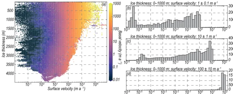
The ice-sheet model could, in theory, be used to predict ero-sion at candidate drill sites; however, the 40 km grid resolu-tion is too coarse for this purpose, given that drill sites will likely be located near nunataks where topographic relief is high. Even if the model was run at higher resolution, insuf-ficient knowledge of the geothermal heat flux and other fac-tors that influence basal conditions would preclude accurate erosion predictions. Instead we use the model as a guide to the relationship among three factors: ice thickness, surface velocity, and basal velocity (Fig. 4). Thickness and surface
velocity are known or easily measured, while basal veloc-ity, a strong indicator of erosion or preservation, is generally unknown or difficult to infer from measurements. Figure 4 shows that at the depths of interest for subglacial drilling in West Antarctica (up to∼1 km), significant glacial erosion is unlikely in areas where the surface velocity is less than ∼10 m yr−1. Such areas are common in the ice-sheet inte-rior, as well as in some areas near the margin (Fig. 1). This result is consistent with other ice-sheet model experiments investigating the distribution of subglacial erosion in Antarc-tica (Jamieson et al., 2010).
Although slow-flowing ice is present near many of the can-didate drill sites shown in Fig. 1, the lowest velocities occur at the ice divides in the interior, near sites such as the Whit-more Mountains and Mt. Woollard. At these interior sites, where (i) surface temperatures are very low and (ii) ice ei-ther thickened modestly during glacial periods (Ackert et al., 1999, 2007; Sect. 5) or potentially thinned in some areas (Fig. 2), subglacial drill targets, to depths of at least a few hundred meters, have likely remained continuously frozen. This is supported by field observations and exposure dating at the Pirrit Hills, Ohio Range, Nash Hills, and Whitmore Mountains (Ackert et al., 2007; Mukhopadhyay et al., 2012; Sect. 5), which show that bedrock surfaces near the modern ice level are commonly weathered and have exposure ages of hundreds of thousands of years, implying that preserved bedrock surfaces likely extend below modern ice levels.
Sites near the modern ice-sheet margin, such as Haag Nunataks, Mt. Murphy, and the Jones Mountains, are pre-dicted to thicken by up to∼800–1000 m during glacial peri-ods (Fig. 2), which suggests that bedrock surfaces there may be vulnerable to erosion beneath thick ice that is sliding at its base. Geologic constraints on former highstands are not available at these sites; however field observations from a site near Mt. Murphy indicate that ice was at least∼300 m thicker than present during the LGM (Johnson et al., 2008). Of all the candidate sites that are located near the coast, the most extensive investigation of former ice cover has been conducted at the Ford Ranges (Stone et al., 2003; Sugden et al., 2005), a group of peaks which extend∼100 km inland from the modern grounding line (Fig. 1) and span multiple grid cells in the ice-sheet model. The model predicts mod-erate thickening during glacial periods at the upstream edge of the Ford Ranges (Fig. 2s), but considerably more near the modern grounding line (up to∼900 m; not shown in Fig. 2), which is consistent with geologic constraints on LGM ice levels (Stone et al., 2003). Sugden et al. (2005) reported ev-idence of wet-based glacial erosion on the lower flanks of many of the peaks in the Ford Ranges, especially those clos-est to the modern grounding line. Therefore, if uneroded sub-glacial bedrock surfaces exist here, they will most likely be found at shallow depths near the inland peaks, where past thickening was more limited and ice velocities are lower.
10-1 100 101 102 103 104
10-4
10-5
10-6 10-3 10-2 10-1 100 101 102
10-4
10-5
10-6 10-3 10-2 10-1 100 101 102
10-4
10-5
10-6 10-3 10-2 10-1 100 101 102
Surface velocity (m a-1)
Basal velocity (m a-1)
500 1000 1500 2000 2500 3000 3500 4000
Ice thickness (m)
0.01 0.1 1 10 100 1000 1000
Basal velocity (m a
-1
)
0 100 200 300 (a)
(b)
0 1000 2000 3000 4000
Number of points
0 5000 10 000 15 000 20 000 (c)
(d)
Ice thickness: 0–1000 m; surface velocity: 1 ± 0.1 m a-1
Ice thickness: 0–1000 m; surface velocity: 10 ± 1 m a-1
Ice thickness: 0–1000 m; surface velocity: 100 ± 10 m a-1
Figure 4. (a)The relationship between surface velocity, ice thickness, and basal velocity, as predicted by the 5 Myr ice-sheet model. Results for the full ice sheet are binned by surface velocity and ice thickness, and each bin is colored by its average basal velocity. This averaging hides considerable variability in the actual range of basal velocities within each bin. Therefore, in panels(b)–(d), we provide histograms of basal velocity for points in the model where the ice is less than 1000 m thick, for surface velocities of∼1,∼10, and∼100 m yr−1. At depths relevant to subglacial drilling, significant subglacial erosion is unlikely in areas where the surface velocity is less than∼10 m yr−1 (see Fig. 1).
the Pensacola Mountains (Fig. 1), show evidence for sur-face preservation by cold-based ice cover (Balco et al., 2016; Bentley et al., 2017). Additionally, radar data over ice rises around the perimeter of Antarctica indicate that the majority of them are currently frozen to their beds (Matsuoka et al., 2015). Although this was not necessarily the case during past glacial periods, the radar data indicate that cold-based ice may, in fact, be common near slow-flowing areas of the ice-sheet margin. Taken together, these observations indicate that although preserved subglacial bedrock surfaces likely exist at some coastal sites, it may be challenging to predict their lo-cations with confidence.
4.4 Bedrock lithology
With the possible exception of Mt. Resnik, which is fully ice covered, the sites shown in Figs. 1 and 2 all have quartz-bearing bedrock that would allow for measurements of a wide range of cosmogenic nuclides. However, at some sites, the exposed rock also includes lithologies in which the ability to make cosmogenic-nuclide measurements would be lim-ited, or, in some cases, impossible. These sites are the Nash Hills (see Sect. 5), Mt. Petras (Spiegel et al., 2016), the Jones Mountains (Rutford and McIntosh, 2007), and Mt. Johns (Storey and Dalziel, 1987). Drilling at these sites may there-fore remain risky unless the subglacial distribution of rock types can be determined.
5 Drill site reconnaissance
As discussed in Sect. 2 there are advantages to drilling in the neighborhood of exposed nunataks. However, the effects of
nunataks on the local ice flow and meteorology cannot be captured at the scale of the ice-sheet model used in Sects. 3 and 4, introducing considerations that need to be addressed by field reconnaissance. Fieldwork prior to drilling also al-lows for (i) sampling of exposed bedrock to test its antiq-uity with cosmogenic-nuclide measurements, (ii) determin-ing the limits of glacial-to-present ice-sheet fluctuation, (iii) examining weathering features for evidence of rock surface preservation, and (iv) locating potential drill sites using ice-penetrating radar.
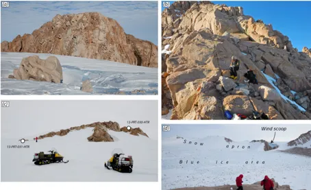
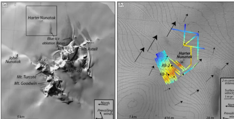
Figure 5. (a)Bedrock ridge located southeast of Mt. Axtell at the Pirrit Hills (Fig. 6). The granite is oxidized and displays large cavernous weathering pits (ice axe in foreground for scale). Such weathering features are common at the Pirrit Hills, both on higher mountain flanks and intersecting the modern ice surface as shown here.(b)Photo looking up the NE ridge of Mt. Axtell. Glacially deposited boulders rest on the more oxidized bedrock of the ridge. The depositional limit is∼15 m above the boulders in the foreground.(c)Photo of Harter Nunatak, showing the location of bedrock samples collected for cosmogenic-nuclide measurements. (d)Backside of the bedrock ridge shown in panel(a). The ridge is orthogonal to the surface winds. Ice levels on the upwind side of the ridge are∼90–130 m higher than at the blue-ice ablation zone in the lee. The ridge is directly flanked by a wind scoop on its upwind side (not visible in panela) and a snow apron on its downwind side.
grounding line, where regional ice flow velocities are less than 5 m yr−1 (Rignot et al., 2011). Here we were able to obtain evidence of low bedrock erosion, sizable glacial– interglacial fluctuations in ice cover, and radar profiles that revealed potential drill sites. Based on these and other fac-tors discussed below, we chose to drill at two sites near Har-ter Nunatak, a minor outcrop∼5 km north of the Pirrit Hills massif.
5.1 Evidence for exposure and preservation of subglacial bedrock surfaces
At the Pirrit Hills, minimally weathered glacial deposits were found up to∼330 m above the modern ice surface, marking the LGM highstand. This is similar to the thickening pre-dicted by the ice-sheet model (Fig. 2f). Despite this evidence for thicker ice, there is almost no indication of recent glacial erosion. Bedrock surfaces are oxidized, and, in places, ex-hibit case hardening, wind polish, and cavernous weathering pits (Fig. 5). Weathered surfaces occur both high on moun-tain flanks as well as near the modern ice surface, where
they commonly intersect and appear to descend below the ice. Similar evidence for lower ice levels in the past has been found in other parts of East and West Antarctica (Mercer, 1968; Lilly et al., 2010; Mukhopadhyay et al., 2012). Al-though these observations demonstrate that ice levels were lower in the past, they establish neither the magnitude nor the timing of thinning.
We collected two samples of weathered bedrock from Har-ter Nunatak (Figs. 6, 7) for analysis of cosmogenic10Be and
26Al to determine the exposure, ice cover, and erosional
Figure 6. (a)WorldView satellite imagery (copyright DigitalGlobe, Inc.) of the Pirrit Hills. Bright areas on the ice sheet generally correspond to areas of steeper surface slopes and overlie or are in the lee of subglacial ridges. The black box shows the location of panel(b).(b)Map of Harter Nunatak (center) and the surrounding area. Elevation contours are derived from WorldView satellite imagery (DEM created by the Polar Geospatial Center). Colors represent ice thickness as measured with the GSSI radar system and arrows represent ice velocity as measured by repeat stake surveys (refer to the Appendix for measurement details). The location of the radar profile in Fig. 8 is not shown on this map, but it intersects the RB-2 borehole and is oriented approximately perpendicular to the ice-flow direction. The ice velocity measured closest to the RB-2 drill site is∼0.25 m yr−1. Changes in ice-surface elevation were also measured at these stakes. The winds flow from the southwest, but are forced to diverge around the Pirrit Hills. The range of wind directions shown in panel(a)reflects the fact that the wind orientation varies with location around the mountains. The wind direction is relatively constant within the domain of panel(b)and so a single vector is used to represent the wind direction.
Firn temperatures in the vicinity of the Pirrit Hills are ap-proximately −26◦C and the ice is undoubtedly frozen to bedrock within a few hundred meters of the surface. Increas-ing ice thickness by∼330 m during the LGM is unlikely to have raised basal temperatures to near melting. As discussed below, ice surface velocities at the site where we ultimately decided to drill are<1 m yr−1. Given the expected relation between surface velocity, ice thickness, and basal velocity shown in Fig. 4, this suggests that uneroded bedrock surfaces likely extend hundreds of meters below the modern ice level.
5.2 Local meteorology, accumulation, and ablation As noted above, mean annual temperature in the region of the Pirrit Hills is approximately −26◦C. Firn depths vary from zero over blue-ice areas to at least ∼36 m, as mea-sured in access holes for subglacial drilling described below. Ice-motion stakes placed around Harter Nunatak in 2015 and resurveyed 1 year later in 2016 (Fig. 6) showed changes in the ice surface of±0.4 m, comparable to the height of sas-trugi in the area. Given these values, accumulation in the vicinity of the nunatak appears to be low, suggesting that the firn and ice column overlying the targeted drill sites accumu-lated upstream, but nearby.
Regionally, snow-bearing winds descend the ice sheet and cross the Pirrit Hills from southwest to northeast. Snow has
accumulated into an embankment upwind of the Pirrit Hills, which rises over a distance of∼5–10 km to the level of the col between Mt. Tidd and Mt. Goodwin (Fig. 6a). The ice surface drops∼600 m across this obstruction to the north-east, where the massif is bordered by a 1–2 km wide blue-ice ablation zone. This geometry results from descending warm, turbulent, foehn-like winds that ablate the ice surface in the lee of the mountains (see Bintanja, 1999). Any changes in wind direction during collapse events could modify this pat-tern of accumulation and ablation and potentially induce ice-thickness changes comparable to amounts expected from dy-namical thinning (Fig. 2). Atmospheric modeling suggests that surface winds near the Pirrit Hills may vary slightly in di-rection and magnitude during collapse events (Scherer et al., 2016); however a fundamental reconfiguration of accumula-tion and ablaaccumula-tion areas appears unlikely.
0 0.5 1 1.5 2 0.2
0.4 0.6 0.8 1
250 500 750 1000 200
500 750
1000 1500
2000 3000
5000 Min. cumulative exposure (kyr)
Min. cumulative ice cover (kyr)
Figure 7.10Be and26Al data for the bedrock samples from Harter Nunatak shown in Fig. 5c. Nuclide concentrations are normalized to the surface production rate for each sample (N∗=N/P, where N is the10Be or26Al concentration andP is the local production rate of that nuclide). Ellipses represent 1σuncertainty regions. Con-tinuously exposed and uneroded surfaces will plot along the black line near the top. Continuously exposed and eroding surfaces will plot between the black line and the solid gray line. Samples plot-ting below the solid gray line, such as those from Harter Nunatak, require at least one episode of ice cover following prior exposure. Dashed contours show lower limits on the cumulative exposure and cumulative ice cover experienced by the samples.
probably best avoided by targeting the crests of subglacial ridges.
5.3 Selected drill sites near Harter Nunatak
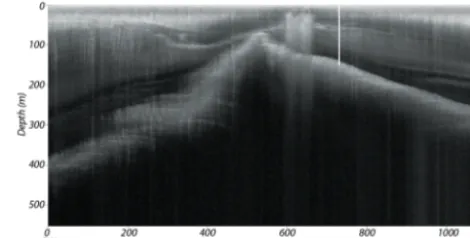
The subglacial topography northeast of the Pirrit Hills ap-pears to be that of a large cirque, its central basin flanked by subglacial ridges descending from Mt. Tidd and Mt. Turcotte and re-emerging at Harter and John nunataks, respectively (Fig. 6). Regional ice flow crosses these ridges obliquely from west to east, producing steep, locally crevassed slopes along much of their length, precluding drilling into the un-derlying bedrock. However, in the course of radar recon-naissance in 2013 we circled both outlying nunataks and identified a subglacial ridge extending northwest of Harter Nunatak. Unlike the major ridges radiating from the Pirrit Hills massif, this ridge lies roughly parallel to ice flow and is overlain by a featureless firn surface dipping gently towards the nunatak. As shown in Fig. 8, the ridge is asymmetric with steeply dipping southwest and gently dipping (∼20◦) north-east flanks. This ridge became the chosen target for two drill holes in 2016–2017. Radar methods and additional survey data are given in the Appendix.
The trend in the ridge crest (Fig. 6) is almost perpendicular to the prevailing wind direction. Combined with the steep-ness of the upwind face, this might be expected to lead to a
Figure 8.Unmigrated radar profile collected with the CReSIS radar showing the location of the 150 m RB-2 borehole to the bed. Profile is oriented perpendicular to the ridge.
lee-side ablation zone in any deglaciation that removed hun-dreds of meters of regional ice, mimicking the gross mor-phology of ice surfaces around the Pirrit Hills discussed above. However, smaller deglaciations that only exposed tens of meters of the ridge crest may have left a lee-side snow-bank, similar to that downwind of Harter Nunatak at the present day. In siting a shallow subglacial drill hole here, we therefore aimed to drill into the crest of the ridge itself.
and Möller Ice Stream, deglaciated in the past. Because we were unable to recover bedrock from a shallower site, the measurements will not necessarily be able to detect deglacia-tions in which less than 150 m of thinning occurred.
6 Conclusions
Measurements of cosmogenic nuclides in bedrock retrieved from below the WAIS have the potential to establish whether and when marine-based portions of the ice sheet deglaciated in the past. The potential of this method, however, requires that drill sites meet three basic criteria: (i) local ice levels must be drawn down significantly during collapse events, (ii) the subglacial bedrock must contain minerals in which useful cosmogenic nuclides can be measured, and (iii) the cosmogenic-nuclide record, which is primarily produced in the top few meters of exposed bedrock, must remain contin-uously protected from erosion. These criteria are also appli-cable to subglacial drilling projects testing whether marine basins in East Antarctica deglaciated in the past. Sites that are expected to be most indicative of past ice-sheet extent are located adjacent to deep marine basins, such as Bentley Sub-glacial Trench, where maximum ice loss would occur during a collapse event. Because ice levels at each of the potential drill sites discussed above are sensitive to the deglaciation of different sectors of the WAIS, subglacial samples from mul-tiple sites will ultimately be required to fully determine the configuration of the ice sheet during past interglacial periods.
The Pirrit Hills are located in the Weddell Sea sector, midway between the grounding line and the divide. Ice-sheet modeling suggests that deglaciation of Robin Sub-glacial Basin induces thinning of a few hundred meters at the Pirrit Hills. Field observations and cosmogenic-nuclide measurements indicate that ice levels at this site have, in-deed, been lower in the past, and multiple lines of evidence suggest that uneroded bedrock extends hundreds of meters below the modern ice surface. Ice-penetrating radar surveys revealed a gently plunging subglacial ridge extending from nearby Harter Nunatak, and, in the 2016–2017 summer, an 8 m bedrock core was extracted from the ridge from below 150 m of ice. If ice levels at the drill site are representative of the region, measurements on the core should constrain past drawdowns of grounded ice in the Weddell Sector of the ice sheet.
Appendix A: Geochemical and geophysical measurements
A1 10Be and26Al measurements
Samples were prepared for10Be/9Be and26Al/Al measure-ments at the University of Washington. We crushed the rock samples, sieved them at 250–500 µm, and purified quartz us-ing surfactants and dilute hydrofluoric acid etchus-ing (Kohl and Nishiizumi, 1992). Samples were then dissolved in hydroflu-oric acid, after which total Al concentrations were measured on aliquots of the solution via inductively coupled plasma op-tical emission spectrometry. Be and Al were isolated using ion-exchange chromatography (Ditchburn and Whitehead, 1994), and Be and Al isotope ratios were measured at the Lawrence Livermore National Laboratory Center for Accel-erator Mass Spectrometry (LLNL-CAMS). Be isotope ratios were measured relative to the ICN 01-5-4 Be standard, as-signed a10Be/9Be ratio of 2.851×10⁻¹²by Nishiizumi et al. (2007). We compute production rates for10Be and26Al using the method of Lifton et al. (2014) as implemented in the ver-sion 3 exposure age calculator (Balco et al., 2008). Produc-tion rates are calibrated from the CRONUS-Earth primary calibration data sets (Borchers et al., 2016). Atmospheric pressure at sample sites is calculated using the relation be-tween elevation and Antarctic atmospheric pressure of Stone (2000). Production by muons is calculated using the method of Balco (2017).
A2 Ice-penetrating radar surveys
We used a radar built by the Center for Remote Sensing of Ice Sheets (CReSIS) with a center frequency of 750 MHz. This radar has a cross-track antenna array consisting of two widely spaced transmitters and eight receivers designed to identify and locate off-nadir reflections. After processing, a full tomographic reconstruction of the subglacial topogra-phy was constructed. However, prior to the 2016–2017 sub-glacial drilling season at the Pirrit Hills, ice-thickness errors were discovered in this reconstruction, and so the bed at the drill site was re-surveyed with a Geophysical Survey Systems Inc. (GSSI) SIR-4000 control unit and a 100 MHz monostatic transceiver. These data are shown in Fig. 6b. The survey
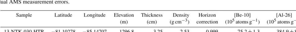
Table A1.Sample information and cosmogenic-nuclide concentrations. Errors (±1σ) include laboratory procedural uncertainties and indi-vidual AMS measurement errors.
Sample Latitude Longitude Elevation Thickness Density Horizon [Be-10] [Al-26] (m) (cm) (g cm−3) correction (105atoms g−1) (105atoms g−1)
13-NTK-030-HTR −81.10278 −85.14707 1296.8 3.25 2.53 0.999 75.2±1.3 384.9±8.8 13-NTK-031-HTR −81.10242 −85.14913 1290.1 1.75 2.58 0.998 73.6±0.97 354.9±7.8
consisted of parallel lines spaced 50 m apart and oriented obliquely to the subglacial ridge, as well as other exploratory lines around Harter Nunatak. The survey was conducted by towing the antenna on foot at a pace of less than 0.5 m s−1. The data were processed using GSSI RADAN software. Dis-tance and elevation corrections were applied to the data. To reduce noise, the data were stacked and a bandpass filter was applied. To calibrate radar wave propagation velocities and thereby improve ice-thickness estimates, we measured firn density to a depth of 38 m and used the relationship of Ko-vacs et al. (1995) to estimate how the real dielectric con-stant varied with depth. We extrapolated the depth–density relationship to deeper depths by fitting the data using a firn-densification model (Herron and Langway, 1980). Drilling at the RB-2 site (Fig. 6b) encountered the bed at a depth of 150 m, confirming ice-thickness estimates from radar sur-veys of 152±10 m.
A3 Strain and accumulation measurements
A total of 16 stakes were arranged in a grid around Harter Nunatak, and two additional stakes were placed over the sub-glacial ridge (Fig. 6b). Stakes were installed and surveyed in December 2015, and measurements were repeated in Decem-ber 2016. Stake positions were surveyed with a Trimble 5700 GPS receiver with a Zephyr Geodetic antenna. No base sta-tion was used for the first survey; the second survey was able to use a POLENET GPS station located on Harter Nunatak as a base station. Mean velocity uncertainty is 0.23 m yr−1.
Change in snow surface height was measured at each stake. Over the 1-year period, height change varied from−39 to+43 cm yr−1, with a mean of−5 cm yr−1. There is no
Competing interests. The authors declare that they have no conflict of interest.
Acknowledgements. Support for this work was provided through US National Science Foundation (NSF) grants 1142162 and 1341728 and the United States Antarctic Program. Perry Spector received funding from the NSF Graduate Research Fellowship Program. We thank Maurice Conway and Paul Koubek for assis-tance in the field, Seth Campbell for guidance in collection and processing of radar data, and Taryn Black and Mika Usher for field and laboratory assistance. Geospatial support for this work provided by the Polar Geospatial Center under NSF OPP awards 1043681 and 1559691.
Edited by: Arjen Stroeven
Reviewed by: Nathaniel A. Lifton and one anonymous referee
References
Ackert, R. P., Barclay, D. J., Borns, H. W., Calkin, P. E., Kurz, M. D., Fastook, J. L., and Steig, E. J.: Measurements of past ice sheet elevations in interior West Antarctica, Science, 286, 276– 280, 1999.
Ackert, R. P., Mukhopadhyay, S., Parizek, B. R., and Borns, H. W.: Ice elevation near the West Antarctic Ice Sheet divide during the last glaciation, Geophys. Res. Lett., 34, L21506, https://doi.org/10.1029/2007GL031412, 2007.
Alley, R. B., Anandakrishnan, S., Christianson, K., Horgan, H. J., Muto, A., Parizek, B. R., Pollard, D., and Walker, R. T.: Oceanic forcing of ice-sheet retreat: West Antarctica and more, Annu. Rev. Earth Pl. Sc., 43, 207–231, 2015.
Anderson, J. B., Warny, S., Askin, R. A., Wellner, J. S., Bohaty, S. M., Kirshner, A. E., Livsey, D. N., Simms, A. R., Smith, T. R., Ehrmann, W., Lawver, L. A., Barbeau, D., Wise, S. W., Kulhanek, D. K., Weaver, F. M., and Majewski, W.: Progressive Cenozoic cooling and the demise of Antarctica’s last refugium, P. Natl. Acad. Sci. USA, 108, 11356–11360, 2011.
Ashworth, A. C. and Erwin, T. L.: Antarctotrechus balli sp. n. (Carabidae, Trechini): the first ground beetle from Antarctica, ZooKeys, 635, 109–122, 2016.
Balco, G.: Production rate calculations for cosmic-ray-muon-produced10Be and 26Al benchmarked against geological cali-bration data, Quat. Geochronol., 39, 150–173, 2017.
Balco, G., Stone, J. O., Lifton, N. A., and Dunai, T. J.: A com-plete and easily accessible means of calculating surface exposure ages or erosion rates from10Be and26Al measurements, Quat. Geochronol., 3, 174–195, 2008.
Balco, G., Stone, J. O., Sliwinski, M. G., and Todd, C.: Features of the glacial history of the Transantarctic Mountains inferred from cosmogenic26Al,10Be and21Ne concentrations in bedrock surfaces, Antarct. Sci., 26, 708–723, 2014.
Balco, G., Todd, C., Huybers, K., Campbell, S., Vermeulen, M., Hegland, M., Goehring, B. M., and Hillebrand, T. R.: Cosmogenic-nuclide exposure ages from the Pensacola Moun-tains adjacent to the Foundation Ice Stream, Antarctica, Am. J. Sci., 316, 542–577, 2016.
Bamber, J. L., Riva, R. E., Vermeersen, B. L., and LeBrocq, A. M.: Reassessment of the potential sea-level rise from a collapse of the West Antarctic Ice Sheet, Science, 324, 901–903, 2009. Barnes, D. K. and Hillenbrand, C.-D.: Faunal evidence for a
late Quaternary trans-Antarctic seaway, Glob. Change Biol., 16, 3297–3303, 2010.
Behrendt, J., Finn, C., Morse, D., and Blankenship, D.: One hun-dred negative magnetic anomalies over the West Antarctic Ice Sheet (WAIS), in particular Mt. Resnik, a subaerially erupted vol-canic peak, indicate eruption through at least one field reversal, in: Antarctica: A Keystone in a Changing World, Proceedings of the 10th International Symposium on Antarctic Earth Sciences, Extended Abstract 030, 1–4, 2007.
Behrendt, J. C., Blankenship, D. D., Finn, C. A., Bell, R. E., Sweeney, R. E., Hodge, S. M., and Brozena, J. M.: CASERTZ aeromagnetic data reveal late Cenozoic flood basalts (?) in the West Antarctic rift system, Geology, 22, 527–530, 1994. Bentley, M. J., Hein, A., Sugden, D., Whitehouse, P., Shanks, R.,
Xu, S., and Freeman, S.: Deglacial history of the Pensacola Mountains, Antarctica from glacial geomorphology and cosmo-genic nuclide surface exposure dating, Quaternary Sci. Rev., 158, 58–76, 2017.
Bierman, P. R., Corbett, L. B., Graly, J. A., Neumann, T. A., Lini, A., Crosby, B. T., and Rood, D. H.: Preservation of a preglacial landscape under the center of the Greenland Ice Sheet, Science, 344, 402–405, 2014.
Bintanja, R.: On the glaciological, meteorological, and climatolog-ical significance of Antarctic blue ice areas, Rev. Geophys., 37, 337–359, 1999.
Borchers, B., Marrero, S., Balco, G., Caffee, M., Goehring, B., Lifton, N., Nishiizumi, K., Phillips, F., Schaefer, J., and Stone, J.: Geological calibration of spallation production rates in the CRONUS-Earth project, Quat. Geochronol., 31, 188–198, 2016. Briggs, R. D., Pollard, D., and Tarasov, L.: A data-constrained large ensemble analysis of Antarctic evolution since the Eemian, Qua-ternary Sci. Rev., 103, 91–115, 2014.
Bromley, G. R., Hall, B. L., Stone, J. O., and Conway, H.: Late Pleistocene evolution of Scott Glacier, southern Transantarc-tic Mountains: implications for the AntarcTransantarc-tic contribution to deglacial sea level, Quaternary Sci. Rev., 50, 1–13, 2012. de Boer, B., Dolan, A. M., Bernales, J., Gasson, E., Goelzer, H.,
Golledge, N. R., Sutter, J., Huybrechts, P., Lohmann, G., Ro-gozhina, I., Abe-Ouchi, A., Saito, F., and van de Wal, R. S. W.: Simulating the Antarctic ice sheet in the late-Pliocene warm period: PLISMIP-ANT, an ice-sheet model intercomparison project, The Cryosphere, 9, 881–903, https://doi.org/10.5194/tc-9-881-2015, 2015.
DeConto, R. M. and Pollard, D.: Contribution of Antarctica to past and future sea-level rise, Nature, 531, 591–597, 2016.
Ditchburn, R. G. and Whitehead, N. E.: The separation of10Be from silicates, in: Third Workshop of the South Pacific Environmen-tal Radioactivity Association, edited by: Hancock, G. and Wall-brink, P., Australian National University, Canberra, 4–7, 1994. Dunbar, N. W., McIntosh, W. C., and Esser, R. P.: Physical setting
and tephrochronology of the summit caldera ice record at Mount Moulton, West Antarctica, Geol. Soc. Am. Bull., 120, 796–812, 2008.
to polar ice-sheet mass loss during past warm periods, Science, 349, https://doi.org/10.1126/science.aaa4019, 2015.
Feldmann, J. and Levermann, A.: Collapse of the West Antarctic Ice Sheet after local destabilization of the Amundsen Basin, P. Natl. Acad. Sci. USA, 112, 14191–14196, 2015.
Fretwell, P., Pritchard, H. D., Vaughan, D. G., Bamber, J. L., Bar-rand, N. E., Bell, R., Bianchi, C., Bingham, R. G., Blanken-ship, D. D., Casassa, G., Catania, G., Callens, D., Conway, H., Cook, A. J., Corr, H. F. J., Damaske, D., Damm, V., Ferracci-oli, F., Forsberg, R., Fujita, S., Gim, Y., Gogineni, P., Griggs, J. A., Hindmarsh, R. C. A., Holmlund, P., Holt, J. W., Jacobel, R. W., Jenkins, A., Jokat, W., Jordan, T., King, E. C., Kohler, J., Krabill, W., Riger-Kusk, M., Langley, K. A., Leitchenkov, G., Leuschen, C., Luyendyk, B. P., Matsuoka, K., Mouginot, J., Nitsche, F. O., Nogi, Y., Nost, O. A., Popov, S. V., Rignot, E., Rippin, D. M., Rivera, A., Roberts, J., Ross, N., Siegert, M. J., Smith, A. M., Steinhage, D., Studinger, M., Sun, B., Tinto, B. K., Welch, B. C., Wilson, D., Young, D. A., Xiangbin, C., and Zirizzotti, A.: Bedmap2: improved ice bed, surface and thickness datasets for Antarctica, The Cryosphere, 7, 375–393, https://doi.org/10.5194/tc-7-375-2013, 2013.
Fudge, T., Markle, B. R., Cuffey, K. M., Buizert, C., Taylor, K. C., Steig, E. J., Waddington, E. D., Conway, H., and Koutnik, M.: Variable relationship between accumulation and temperature in West Antarctica for the past 31,000 years, Geophys. Res. Lett., 43, 3795–3803, 2016.
Golledge, N. R., Fogwill, C. J., Mackintosh, A. N., and Buckley, K. M.: Dynamics of the last glacial maximum Antarctic ice-sheet and its response to ocean forcing, P. Natl. Acad. Sci. USA, 109, 16052–16056, 2012.
Golledge, N. R., Thomas, Z. A., Levy, R. H., Gasson, E. G. W., Naish, T. R., McKay, R. M., Kowalewski, D. E., and Fogwill, C. J.: Antarctic climate and ice-sheet configuration during the early Pliocene interglacial at 4.23 Ma, Clim. Past, 13, 959–975, https://doi.org/10.5194/cp-13-959-2017, 2017.
Goodge, J. W. and Severinghaus, J. P.: Rapid Access Ice Drill: a new tool for exploration of the deep Antarctic ice sheets and sub-glacial geology, J. Glaciol., 62, 1049–1064, 2016.
Herron, M. M. and Langway, C. C.: Firn densification: an empirical model, J. Glaciol., 25, 373–385, 1980.
Jamieson, S. S., Sugden, D. E., and Hulton, N. R.: The evolution of the subglacial landscape of Antarctica, Earth Planet. Sc. Lett., 293, 1–27, 2010.
Johnson, J. S., Bentley, M. J., and Gohl, K.: First exposure ages from the Amundsen Sea embayment, West Antarctica: The Late Quaternary context for recent thinning of Pine Island, Smith, and Pope Glaciers, Geology, 36, 223–226, 2008.
Jordan, T. A., Ferraccioli, F., Ross, N., Corr, H. F., Leat, P. T., Bing-ham, R. G., Rippin, D. M., le Brocq, A., and Siegert, M. J.: Inland extent of the Weddell Sea Rift imaged by new aerogeophysical data, Tectonophysics, 585, 137–160, 2013.
Joughin, I., Smith, B. E., and Medley, B.: Marine ice sheet col-lapse potentially under way for the Thwaites Glacier Basin, West Antarctica, Science, 344, 735–738, 2014.
Kohl, C. and Nishiizumi, K.: Chemical isolation of quartz for mea-surement of in-situ-produced cosmogenic nuclides, Geochim. Cosmochim. Ac., 56, 3583–3587, 1992.
Korotkikh, E. V., Mayewski, P. A., Handley, M. J., Sneed, S. B., Introne, D. S., Kurbatov, A. V., Dunbar, N. W., and McIntosh,
W. C.: The last interglacial as represented in the glaciochemi-cal record from Mount Moulton Blue Ice Area, West Antarctica, Quaternary Sci. Rev., 30, 1940–1947, 2011.
Kovacs, A., Gow, A. J., and Morey, R. M.: The in-situ dielectric constant of polar firn revisited, Cold Reg. Sci. Technol., 23, 245– 256, 1995.
Laskar, J., Robutel, P., Joutel, F., Gastineau, M., Correia, A., and Levrard, B.: A long-term numerical solution for the insolation quantities of the Earth, Astron. Astrophys., 428, 261–285, 2004. Lewis, A. R., Marchant, D. R., Ashworth, A. C., Hedenäs, L., Hem-ming, S. R., Johnson, J. V., Leng, M. J., Machlus, M. L., Newton, A. E., Raine, J. I., Willenbring, J. K., Williams, M., and Wolfe, A. P.: Mid-Miocene cooling and the extinction of tundra in con-tinental Antarctica, P. Natl. Acad. Sci. USA, 105, 10676–10680, 2008.
Lifton, N., Sato, T., and Dunai, T. J.: Scaling in situ cosmogenic nu-clide production rates using analytical approximations to atmo-spheric cosmic-ray fluxes, Earth Planet Sc. Lett., 386, 149–160, 2014.
Lilly, K., Fink, D., Fabel, D., and Lambeck, K.: Pleistocene dynam-ics of the interior East Antarctic ice sheet, Geology, 38, 703–706, 2010.
Lisiecki, L. E. and Raymo, M. E.: A Pliocene-Pleistocene stack of 57 globally distributed benthicδ18O records, Paleoceanography, 20, PA1003, https://doi.org/10.1029/2004PA001071, 2005. Matsuoka, K., Hindmarsh, R. C., Moholdt, G., Bentley, M. J.,
Pritchard, H. D., Brown, J., Conway, H., Drews, R., Durand, G., Goldberg, D., Hattermann, T., Kingslake, J., Lenaerts, J. T. M., Martín, C., Mulvaney, R., Nicholls, K. W., Pattyn, F., Ross, N., Scambos, T., and Whitehouse, P. L.: Antarctic ice rises and rumples: Their properties and significance for ice-sheet dynam-ics and evolution, Earth-Sci. Rev., 150, 724–745, 2015. Mercer, J. H.: Glacial geology of the Reedy Glacier area,
Antarc-tica, Geol. Soc. Am. Bull., 79, 471–486, 1968.
Morse, D. L., Blankenship, D. D., Waddington, E. D., and Neu-mann, T. A.: A site for deep ice coring in West Antarctica: results from aerogeophysical surveys and thermo-kinematic modeling, Ann. Glaciol., 35, 36–44, 2002.
Mukhopadhyay, S., Ackert, R. P., Pope, A. E., Pollard, D., and De-Conto, R. M.: Miocene to recent ice elevation variations from the interior of the West Antarctic ice sheet: Constraints from geo-logic observations, cosmogenic nuclides and ice sheet modeling, Earth Planet. Sc. Lett., 337, 243–251, 2012.
Mulvaney, R., Triest, J., and Alemany, O.: The James Ross Is-land and the Fletcher Promontory ice-core drilling projects, Ann. Glaciol., 55, 179–188, 2014.
NEEM community members: Eemian interglacial reconstructed from a Greenland folded ice core, Nature, 493, 489–494, 2013. Nishiizumi, K., Finkle, R. C., Ponganis, K. V., Graf, T., Kohl, C. P.,
and Marti, K.: In situ produced cosmogenic nuclides in GISP2 rock core from Greenland Summit, in: Eos, Transactions of the American Geophysical Union, Abstract OS41B–10, 1996. Nishiizumi, K., Imamura, M., Caffee, M. W., Southon, J. R., Finkel,
R. C., and McAninch, J.: Absolute calibration of10Be AMS stan-dards, Nucl. Instrum. Meth. B, 258, 403–413, 2007.
Pollard, D. and DeConto, R. M.: Modelling West Antarctic ice sheet growth and collapse through the past five million years, Nature, 458, 329–332, 2009.
Pollard, D. and DeConto, R. M.: Description of a hybrid ice sheet-shelf model, and application to Antarctica, Geosci. Model Dev., 5, 1273–1295, https://doi.org/10.5194/gmd-5-1273-2012, 2012a. Pollard, D. and DeConto, R. M.: A simple inverse method for the distribution of basal sliding coefficients under ice sheets, applied to Antarctica, The Cryosphere, 6, 953–971, https://doi.org/10.5194/tc-6-953-2012, 2012b.
Pollard, D., DeConto, R. M., and Alley, R. B.: Potential Antarctic Ice Sheet retreat driven by hydrofracturing and ice cliff failure, Earth Planet. Sc. Lett., 412, 112–121, 2015.
Pollard, D., Chang, W., Haran, M., Applegate, P., and DeConto, R.: Large ensemble modeling of the last deglacial retreat of the West Antarctic Ice Sheet: comparison of simple and ad-vanced statistical techniques, Geosci. Model Dev., 9, 1697–1723, https://doi.org/10.5194/gmd-9-1697-2016, 2016.
Price, S., Conway, H., and Waddington, E.: Evidence for late pleis-tocene thinning of Siple Dome, West Antarctica, J. Geophys. Res.-Earth, 112, F03021, https://doi.org/10.1029/2006JF000725, 2007.
Pritchard, H., Ligtenberg, S., Fricker, H., Vaughan, D., Van den Broeke, M., and Padman, L.: Antarctic ice-sheet loss driven by basal melting of ice shelves, Nature, 484, 502–505, 2012. Raymo, M. E., Kozdon, R., Evans, D., Lisiecki, L., and Ford, H. L.:
The accuracy of mid-Pliocene δ18O-based ice volume and sea level reconstructions, Earth-Sci. Rev., 177, 291–302, 2017. Rignot, E., Mouginot, J., and Scheuchl, B.: Ice flow of the Antarctic
ice sheet, Science, 333, 1427–1430, 2011.
Rutford, R. and McIntosh, W.: Jones Mountains, Antarctica: ev-idence for Tertiary glaciation revisited, in: Antarctica: A Key-stone in a Changing World, Proceedings of the 10th International Symposium on Antarctic Earth Sciences, Extended Abstract 203, 2007.
Scambos, T., Bell, R., Alley, R., Anandakrishnan, S., Bromwich, D., Brunt, K., Christianson, K., Creyts, T., Das, S., DeConto, R., Fricker, H. A., Holland, D., MacGregor, J., Medley, B., Nicolas, J. P., Pollard, D., Siegfried, M. R., Smith, A. M., Steig, E. J., Trusel, L. D., Vaughan, D. G., and Yager, P. L.: How much, how fast?: A science review and outlook for research on the instabil-ity of Antarctica’s Thwaites Glacier in the 21st century, Global Planet. Change, 153, 16–34, 2017.
Schaefer, J. M., Finkel, R. C., Balco, G., Alley, R. B., Caffee, M. W., Briner, J. P., Young, N. E., Gow, A. J., and Schwartz, R.: Green-land was nearly ice-free for extended periods during the Pleis-tocene, Nature, 540, 252–255, 2016.
Scherer, R. P., Aldahan, A., Tulaczyk, S., Possnert, G., Engelhardt, H., and Kamb, B.: Pleistocene collapse of the West Antarctic ice sheet, Science, 281, 82–85, 1998.
Scherer, R. P., DeConto, R. M., Pollard, D., and Alley, R. B.: Wind-blown Pliocene diatoms and East antarctic ice sheet retreat, Nat. Commun., 7, 1–9, https://doi.org/10.1038/ncomms12957, 2016. Schoof, C.: Ice sheet grounding line dynamics: Steady states, sta-bility, and hysteresis, J. Geophys. Res.-Earth, 112, F03S28, https://doi.org/10.1029/2006JF000664, 2007.
Souchez, R., Jouzel, J., Landais, A., Chappellaz, J., Lorrain, R., and Tison, J.-L.: Gas isotopes in ice reveal a vegetated central Green-land during ice sheet invasion, Geophys. Res. Lett., 33, L24503, https://doi.org/10.1029/2006GL028424, 2006.
Spector, P., Stone, J., Cowdery, S. G., Hall, B., Conway, H., and Bromley, G.: Rapid early-Holocene deglaciation in the Ross Sea, Antarctica, Geophys. Res. Lett., 44, 7817–7825, 2017.
Spiegel, C., Lindow, J., Kamp, P. J., Meisel, O., Mukasa, S., Lisker, F., Kuhn, G., and Gohl, K.: Tectonomorphic evolution of Marie Byrd Land–Implications for Cenozoic rifting activity and onset of West Antarctic glaciation, Global Planet. Change, 145, 98– 115, 2016.
Steig, E. J., Fastook, J. L., Zweck, C., Goodwin, I. D., Licht, K. J., White, J. W., and Ackert, R. P.: West Antarctic ice sheet eleva-tion changes, The West Antarctic Ice Sheet: Behavior and Envi-ronment, 75–90, 2001.
Stone, J. O.: Air pressure and cosmogenic isotope production, J. Geophys. Res.-Sol. Ea., 105, 23753–23759, 2000.
Stone, J. O., Balco, G. A., Sugden, D. E., Caffee, M. W., Sass, L. C., Cowdery, S. G., and Siddoway, C.: Holocene deglaciation of Marie Byrd land, west Antarctica, Science, 299, 99–102, 2003. Storey, B. and Dalziel, I.: Outline of the Structural and Tectonic His-tory Of The Ellsworth Mountains-Thiel Mountains Ridge, West Antarctica, Gondwana six: structure, tectonics, and geophysics, 117–128, 1987.
Sugden, D. E., Balco, G., Cowdery, S. G., Stone, J. O., and Sass, L. C.: Selective glacial erosion and weathering zones in the coastal mountains of Marie Byrd Land, Antarctica, Geomorphol-ogy, 67, 317–334, 2005.
Waddington, E., Conway, H., Steig, E., Alley, R., Brook, E., Tay-lor, K., and White, J.: Decoding the dipstick: thickness of Siple Dome, West Antarctica, at the last glacial maximum, Geology, 33, 281–284, 2005.
Weertman, J.: Stability of the junction of an ice sheet and an ice shelf, J. Glaciol., 13, 3–11, 1974.
Wei, L., Raine, J., and Liu, X.: Terrestrial palynomorphs of the Cenozoic Pagodroma Group, northern Prince Charles Moun-tains, East Antarctica, Antarct. Sci., 26, 69–79, 2014.
Wilch, T. I., McIntosh, W., and Dunbar, N.: Late Quaternary vol-canic activity in Marie Byrd Land: Potential 40Ar/39Ar-dated time horizons in West Antarctic ice and marine cores, GSA Bul-letin, 111, 1563–1580, 1999.