www.ocean-sci.net/6/563/2010/ doi:10.5194/os-6-563-2010
© Author(s) 2010. CC Attribution 3.0 License.
Ocean Science
On the numerical resolution of the bottom layer in simulations
of oceanic gravity currents
N. Laanaia, A. Wirth, J. M. Molines, B. Barnier, and J. Verron
LEGI/MEOM/CNRS, Laboratoire des Ecoulements G´eophysiques et Industriels, UMR 5519, BP 53, 38041 Grenoble cedex 9, France
Received: 11 February 2010 – Published in Ocean Sci. Discuss.: 4 March 2010 Revised: 25 May 2010 – Accepted: 26 May 2010 – Published: 8 June 2010
Abstract. The role of an increased numerical vertical reso-lution, leading to an explicit resolution of the bottom Ekman layer dynamics, is investigated. Using the hydrostatic ocean model NEMO-OPA9, we demonstrate that the dynamics of an idealised gravity current (on an inclined plane), is well captured when a few (around five) sigma-coordinate levels are added near the ocean floor. Such resolution allows to con-siderably improve the representation of the descent and trans-port of the gravity current and the Ekman dynamics near the ocean floor, including the important effect of Ekman veer-ing, which is usually neglected in today’s simulations of the ocean dynamics.
Results from high resolution simulations (withσ and z-coordinates) are compared to simulations with a vertical res-olution commonly employed in today’s ocean models. The latter show a downslope transport that is reduced by almost an order of magnitude and the decrease in the along slope transport is reduced six-fold. We strongly advocate for an in-crease of the numerical resolution at the ocean floor, similar to the way it is done at the ocean surface and at the lower boundary in atmospheric models.
Correspondence to: A. Wirth ([email protected])
1 Introduction
The realism of numerical models of the ocean dynamics de-pends on their capability to correctly represent the important processes, at large and also at small scales. The dynamics of gravity currents was identified as a key process governing the strength of the thermohaline circulation and its heat transport from low to high latitudes (Willebrand et al., 2001).
Oceanic gravity currents are small compared to the basin scales in the horizontal and vertical directions, only about 100 km wide and a few hundred metres thick, but they have a substantial impact on the global climate dynamics.
grid of the numerical model, leading to the above mentioned refinement near the surface.
At the ocean floor a similar PBL develops. This feature is, however, rarely reflected in the structure of the vertical reso-lution. To the contrary, the grid size is usually an increasing function of depth, leading to the sparsest resolution at the ocean floor. The PBL dynamics at the ocean floor can not be explicitly represented with such a vertical grid. Please note, that in numerical models of the dynamics of the atmosphere, a grid refinement near the earth’s surface is commonly em-ployed to resolve explicitly a large part of the important pro-cesses at this boundary. The dynamics at the ocean floor is however similarly important and involved, as the dynamics at the ocean surface and at the lower boundary of the atmo-sphere. A large part of the kinetic energy is supposed to be dissipated at the ocean floor representing a major sink of ki-netic energy and an important player in the global energy cycle of the ocean dynamics.
Furthermore, a misrepresentation of the PBL dynamics is worse in the bottom layer than in the surface layer, when the momentum balance is considered. Indeed, at the surface the wind shear is imposed and thus also the corresponding Ekman transport, which means, that even with a bad repre-sentation of the PBL dynamics the overall Ekman transport is correct in magnitude and direction. In the bottom layer, to the contrary, the shear is a function of the velocity field near the bottom. Getting the velocity field wrong also means, that the Ekman transport is wrong in magnitude and direction. It is through the divergence of the Ekman layer transport that the momentum fluxes at the boundaries are communicated to the ocean interior (see e.g. Pedlosky 1998). The need is es-pecially important when the dynamics of gravity currents are considered. It was demonstrated by Willebrand et al. (2001) that the thermohaline circulation of the North Atlantic in nu-merical models is strongly influenced by the local represen-tation of the gravity current dynamics in the Denmark Strait. Many efforts have been made during the last thirty years to parametrise the effect of the bottom PBL on the large-scale ocean dynamics. Parametrisations of varying complexity have been developed to represent various features of the dy-namics of gravity currents (see e.g. Killworth and Edwards, 1999; Xu et al., 2006; Legg et al., 2006, 2008). Today there is no generally accepted parametrisation and the representa-tion of gravity currents is considered a major flaw in today’s state-of-the-art ocean models. Developing a parametrisation of the Ekman layer dynamics, based on linear homogeneous stationary Ekman layer theory might be of limited use in cases where the Ekman layer is neither linear nor homoge-neous nor stationary. Indeed, inertial oscillations and a rapid evolution of the gravity current, make the validity of such parametrisations questionable.
In the present work we explore another direction. Rather than parametrising the total PBL dynamics on the bottom we resolve some of it explicitly, by increasing the resolu-tion near the bottom in the very same way as it is commonly
done near the surface. This refinement can easily be imple-mented in aσ-coordinate grid, available in several numerical models of the ocean circulation. This idea has, so far to the best of our knowledge, not been explored in detail. The im-portance of the vertical resolution in gravity current dynam-ics has already been emphasised by various authors. A fine grid or a grid refinement near the ocean floor was already employed, for example, in Ezer and Weatherly (1990), Win-ton et al. (1998), Jungclaus (1999), Ezer and Mellor (2004); Ezer (2005). But we like to mention that in these publica-tions, although having a high vertical resolution, the Ekman layer dynamics in the PBL is usually not sufficiently resolved and the effect of vertical resolution on the gravity current dy-namics has not been explored in detail. Most recently Legg et al. (2008), varying the vertical viscosity over more than three orders of magnitude rather than the grid resolution, noted that resolving the Ekman layer has a dominant role in de-termining the descent of the gravity current and favours its downslope movement. Their paper also gives a very nice in-troduction to, and a review of, recent results using numerical simulations of gravity current dynamics.
In this work we suggest a vertical resolution in ocean mod-els that represents a compromise between calculation time and representation of the important processes. We focus on the importance of vertical resolution in the representation of the dynamics of gravity currents as: (i) gravity currents are affected by the PBL dynamics on the ocean floor, (ii) gravity currents are important features of the large scale circulation, (iii) they represent a difficult problem to simulate numeri-cally and (iv) they have been thoroughly studied in obser-vations, laboratory experiments, numerical models and an-alytical calculations and the results are discussed in a large number of publications.
The present work is dedicated to the importance of Ekman layer dynamics and its vertical resolution in numerical simu-lations of gravity currents. This vertical resolution is shown to be of paramount importance for the process considered here. The important problem of errors in the horizontal pres-sure gradient inσ-coordinate models, a subject discussed in a large number of publications, is not considered here.
2 Dynamics and representation of the oceanic bottom boundary layer
The dynamics in the PBL at the ocean floor is turbulent. The key parameter of its dynamics is the friction velocity:
u∗=
rτ
ρ, (1)
whereτ is the friction force per unit area exerted by the ocean floor andρis the density of the sea water.
δν≈5ν/u∗and which is governed by laminar viscous dynam-ics. Above this layer the dynamics transits in the buffer layer towards the log-layer, which is a few metres thick and gov-erned by turbulent transfer of inertia. The thickness of the buffer-layer is a function of the roughness of the ocean floor. The transfer of inertia is supposed constant throughout the log-layer and its magnitude also depends on the roughness of the ocean floor. In the fourth layer, at even further distance
δf≈0.2u∗/f, of a few tens of metres above ground, rotation influences the dynamics and a turbulent Ekman layer devel-ops (see Coleman et al., 1990; McWilliams, 2009).
The dynamics in the first three layers can not be explicitly resolved in ocean models even in a far future. The viscous sub-layer is only a few millimetres thick and the buffer- and log-layer are governed by turbulent structures of only a few metres in size in the vertical and horizontal directions. An explicit resolution asks for grid cells of less than one me-tre in all three spatial directions and a time step smaller than one second, requirements which are far from being feasible for basin-scale ocean models, with today’s and tomorrow’s computer resources. The characteristic time scale of the dy-namics in the first three boundary layers is faster than the inverse of the Coriolis parameter, which is a prerequisite for an efficient parametrisation in ocean models. The dynam-ics in the first three bottom layers, viscous-, buffer- and log-layer, is usually parametrised by implementing either: (i) a no slip boundary condition together with an increased verti-cal turbulent viscosity or (ii) a drag force at the lowest grid cell, which depends linearly or quadratically on the veloc-ity at the first grid point from the wall. The actual drag force per unit area in today’s ocean models is often given by F=(cD/ρ)(|u|+c)u, where u is the fluid velocity near the
ocean floor,cDthe drag coefficient depending on the
rough-ness of the ocean floor andcis a velocity representing pro-cesses not explicitly included, as for example the tidal dy-namics. This leads to a linear friction force forucand a quadratic friction force foruc. The problem of parametris-ing the influence of these three layers lies in the determina-tion of the corresponding fricdetermina-tion parameters (see Wirth and Verron, 2009; Wirth, 2010).
We prefer to resolve explicitly a part of the dynamics in the Ekman layer rather than to totally parametrise its influence on the dynamics above. The parametrisation of the Ekman layer dynamics is more subtle due to the veering (turning) of the velocity vector in the Ekman layer. When this effect is omitted, as it is currently in most ocean general circulation models, the friction force is not only wrong in magnitude but also in direction. The focus of the present work is on the numerical resolution of the Ekman layer dynamics at the ocean floor.
3 Idealised oceanic gravity current on the f-Plane 3.1 The physical problem considered
In the experiments presented here we use an idealised ge-ometry, considering an infinite gravity current on an inclined plane with constant slope of 1◦in a rotating frame with a con-stant Coriolis parameterf=1.0313×10⁻⁴s−1. The water in the gravity current is1T=0.2 K colder than the surrounding water, gravity isg=9.8065 ms−2and the thermal expansion coefficient equals 2.0−4K−1. This leads to a reduced gravity
g0=3.9226×10⁻⁴ms−2. In the initial condition the thickness
h(y)has a parabolic shape that is 20 km wide and has a maxi-mum value of 200 m. Initially the velocity is in a geostrophic equilibrium.
When dissipative effects and instability of the gravity cur-rent are ignored the gravity curcur-rent is stationary and travels in the along-slope direction with an average geostrophic ve-locity ofu=(g0/f )tan1◦. It is the friction, transmitted by the PBL dynamics, that is responsible for the evolution of the gravity current. Please note that in the rotating case it is friction that makes the gravity current move down-slope, whereas in the non-rotating gravity current friction opposes the down slope movement. This dynamics has been studied numerically in Wirth (2009) using the non-hydrostatic model HAROMOD introduced in Wirth (2004). We are here con-cerned with the representation of the dynamics in hydrostatic ocean models.
3.2 The mathematical model
In the present research we consider two configurations to study the physical problem described above. The first con-figuration is 2.5 dimensional and the second 3 dimensional. In the 2.5D configuration we only consider the dynamics within a 2 dimensional vertical slice perpendicular to the geostrophic velocity. We do not allow for variations in the long-stream direction. Although the geometry is 2-D all three components of the velocity vector are retained. The 2.5-D configuration has two advantages. First, it suppresses large scale instability of the gravity current and the forma-tion of large scale eddies, which is beneficial to our goal of looking at the influence of small scale processes in the PBL. Second, a detailed study of the influence of resolution is nu-merically more feasible in the less costly 2.5-D configura-tion. The 3-D configuration is then used to verify how the re-sults found in the 2.5-D configuration transfer, qualitatively and quantitatively, to the full 3-D case. That is, we check if the presence of 3-D instabilities and other structures alter the results found in the 2.5-D case.
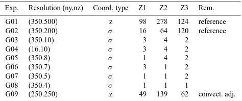
Table 1. List of the 2.5-D exps. The domain spans 50 km in the
y-direction. The number of levels in the vertical zones Z1, Z2 and Z3 (as explained in the text) are given.
Exp. Resolution (ny,nz) Coord. type Z1 Z2 Z3 Rem.
G01 (350.500) z 98 278 124 reference
G02 (350.200) σ 16 64 120 reference
G03 (350.10) σ 3 4 2
G04 (16.10) σ 3 4 2
G05 (350.8) σ 1 4 2
G06 (350.7) σ 3 1 2
G07 (350.5) σ 1 1 2
G08 (350.4) σ 1 1 1
G09 (250.250) z 49 139 62 convect. adj.
The mathematical model used to study the physical con-figuration introduced above comprises the hydrostatic (prim-itive) equations subject to a no slip boundary condition at the bottom and an implicit free surface at the top. The vertical eddy viscosity is 4×10⁻³m2s−1leading to a thickness of the laminar Ekman layer ofδEk=
√
2ν/f=8.8 m and the verti-cal diffusivity is 1×10⁻⁴m2s−1. The horizontal viscosity is
νh=10 m2s−1and the horizontal diffusivity isκh=1 m2s−1.
3.3 The numerical model and its vertical resolution The above introduced mathematical models are numeri-cally integrated with the numerical model NEMO-OPA9 (see Madec, 2008). The horizontal resolution (1y=143 m) in the direction of the slope is, with one exception (1y=3125 m in G04), the same in all experiments (please see Tables 1 and 2 for details). The horizontal resolution of experiment G04 is typical for high resolution regional models. In the three dimensional experiments1x=400 m.
The purpose of our research is to evaluate the effect of a vertical grid refinement near the ocean floor and determine the grid structure that is an optimal compromise between ac-curacy and the cost of calculation. Two types of grid ge-ometries are employed here, both are standard options in the NEMO-OPA9 model. One is the conventional z-coordinate, where all grid-points of a certain level lie at the same depth. The grid structure has a regular orthogonal form. Usually the vertical resolution is a function of depth, with a refine-ment near the surface and a sparse grid at the bottom. For the case considered here, a high resolution at the topography, the refinement has to extend over the total depth, leading to a uniform grid structure with many grid points in areas where they are not necessarily needed.
The second type of grid geometry is the σ-coordinate, which is terrain following. The standard Jacobian formu-lation is used for the calcuformu-lation of the horizontal pressure gradient (see Madec, 2008, 90 p., of the reference manual). In aσ-coordinate model the number of levels is equal every-where so that no grid point is wasted in the vertical. In a
σ-coordinate model grid points of the same level are situated
at the same depth relative to the total depth at each horizon-tal location. This type of grid structure allows for an effi-cient refinement of the grid near the topography. Except for two experiments all our experiments are performed with a
σ-coordinate system. No 3-D reference experiments (high resolution) experiments have been performed due to the in-hibitive computer requirements. The convective adjustment on the tracer (only) is used in all simulations (by increasing the vertical diffusivity to 10 m2s−1).
We want to emphasise here that the mathematical model presented in the previous subsection has a well defined solu-tion which is, of course, independent of the numerical model employed to approach it. As the numerical models with both types of grids are consistent their solutions will both con-verge to the mathematical solution when the grid resolution and the corresponding time step are reduced. The question is, however, which of the grids has a faster convergence when numerical costs are equal. The case considered here is clearly in favour of theσ-coordinate model.
In our numerical simulations we distinguish three zones in the vertical direction (see Fig. 3). The first zone, called Z1, includes the sea-floor PBL and is about 40 m thick. The second, called Z2, extends from about 40 to 200 m from the ocean floor and includes thus the upper part of the vein. The third zone, called Z3, extends from about 200 m above the ocean floor to the surface and contains no gravity current water. It, nevertheless, has an influence on the dynamics of the gravity current. The vertical resolution is varied between experiments in the three zones to explore its effect on the representation of the gravity current dynamics.
4 Experiments
We performed two sets of experiments, the first are 2.5-D and the second 3-D. Both sets are explained in the following two subsections, the results of the experiments are given in the next section. The initial conditions, identical for both sets of experiments, can be seen in Fig. 1, the temperature is constant within the gravity current which has a parabolic shape and the long-slope velocity is geostrophically adjusted, please note that it reverses within the gravity current. 4.1 Experiments 2.5-D
Fig. 1. Initial condition: temperature (left) and geostrophically adjusted velocityu(cross stream component; y-direction is upslope).
the first level is at only 0.3 m from the ocean floor (measured at the upslope side of the domain). Experiment G02 is thus of higher quality than G01 due to the grid refinement near the ocean floor. In other experiments the resolution is varied in the vertical zones defined above (Z1, Z2 and Z3) to evaluate the lack of resolution in the different zones, each one being representative of different physical processes. For the grids with three levels in the zone Z1 the first three horizontal-velocity grid points are at 2.5 m, 10 m and 22.5 m from the ocean floor resolution (on the up slope side of the domain). A typicalσ-coordinate grid with three levels in the zone Z1 is given in Fig. 3
Experiment G04 has a coarser horizontal with
1y=3.125 km a value typical for today’s state-of-the-art regional GCM calculations. A second experiment, G09, with a z-coordinate system is performed. It has a coarser resolution (in x and z) as compared to G01 and the convective adjustment is also used on the momentum (by increasing the vertical viscosity to 10 m2s−1). Such scheme is usually employed in ocean global circulation models (OGCM) integrations to parametrise convective processes at the ocean surface. The convective adjustment procedure used, increases the vertical viscosity and diffusivity many orders of magnitude, to 10 m2s−1, when a static instability
is detected. This mimics convection and is beneficial near the surface, but destroys the gravity current dynamics as we will demonstrate in the next section.
4.2 Experiments 3-D
In the 3-D experiments a reference experiment, as performed for the 2.5-D case, is prohibited by the size of the calculation. We therefore used the resolution in Z1 and Z2, which was found to give good results in the 2.5-D case, experiment G03 (see Table 1 and Sect. 5) as the resolution of our 3-D refer-ence experiment G11 (see Table 2). The higher resolution
Table 2. List of the 3-D exps. (see Table 1 for details).
Exp. Resolution Coord. type Z1 Z2 Z3 (nx,ny,nz)
G11 (500.350.12) σ 3 4 4 G12 (500.350.10) σ 1 4 4 G13 (500.350.14) σ 0 3 10
in the zone Z3 as compared to the 2.5-D experiments is re-quired for the numerical stability of the calculation. Indeed, the eddy dynamics due to large scale instability of the flow, which are suppressed in the 2.5-D calculations, ask for a higher resolution in Z3 (see Sect. 5). The resolution of G11 is shown in Fig. 3.
The effect of a non resolved Ekman layer was studied in experiment G12, its vertical resolution is similar to G05. Ex-periment G13 at an even sparser resolution is close to what is used in classical high vertical-resolution calculations of grav-ity current dynamics and OGCM calculations.
5 Results
5.1 Results 2.5-D
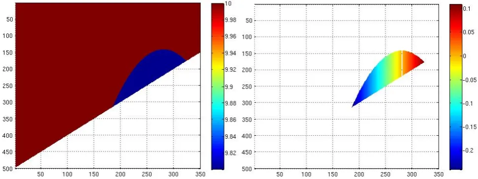
Fig. 2. Temperature structure (in Co) in the reference simulations after 7 days; left: z-coordinate (G01) and right: σ-coordinate (G02). Coordinates give grid in the x-direction and the z-direction for the z-coordinate grid. For theσ-coordinate results are interpolated to the z-coordinate grid (in the z-direction).
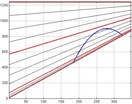
Fig. 3.σ-coordinates of G11 shown (black lines). Red-lines mark the boundaries of the zones Z1, Z2 and Z3 (bottom to top). Blue line gives initial profile of gravity current.
common in all the laboratory experiments and high resolu-tion numerical simularesolu-tions, is a vein, the thick part of the gravity current and a thin “friction layer” at its down slope side. The vein descends only slowly in time, but detrains water at its down-slope side through the friction layer. This two part structure is key to the dynamics of oceanic gravity currents. It is discussed in detail in Wirth (2009).
The first point we like to emphasise is the disastrous effect that the convective adjustment implemented in most ocean models has on the dynamics of gravity currents. When heavier water overlies lighter water a convective dynamics mixes the two water masses in a short time (see e.g. Wirth, 2009). In hydrostatic OGCMs this process is absent and a convective adjustment procedure is used that mixes the two
water masses and their inertia. The convective adjustment used in our simulations does this by artificially augmenting the vertical diffusivity and viscosity to the value of 1 m2s−1. Increasing only the diffusivity and leaving the viscosity un-changed is contrary to the fact that the turbulent Prandtl num-ber is order unity. This procedure is found to mimic very well the convective dynamics at the ocean surface but has a disas-trous effect on the dynamics of gravity currents. Indeed, at the downslope front of the gravity current the down-slope ve-locity decreases in the vicinity of the floor and heavy gravity current water superposes lighter ambient water, which trig-gers convective adjustment. The high vertical viscosity then inhibits a downslope movement of the gravity current and a vertical wall of dense water develops at the down-slope side of the gravity current as shown in Fig. 4, this is an artifact of the convective adjustment procedure. A comparison to Fig. 2 shows clearly the completely different dynamics due to the convective adjustment and demonstrates that it should not be used in gravity current calculations. The experiment involving convective adjustment will not be further discussed in the sequel.
The rate of descent of the gravity current is the most im-portant property, its time evolution is given in Fig. 5. The rate of descent is defined by the movement of the x-component of the centre of gravitycxof the gravity current. It is defined as:
cx=
R
×(T −T0) dA
R
(T −T0) dA
, (2)
whereT0is the temperature of the surrounding water and the
whole area, in the 2.5-D case, or the whole volume, in the 3-D case, is denoted byA.
Fig. 4. Temperature structure (in C◦) in the simulation with convec-tive adjustment (G09). Coordinates give grid levels.
Fig. 5. Down-slope displacement of the centre of gravity of the
gravity current in the 2.5-D experiments during the first 7 days of the experiments. Vertical axis in metres and horizontal axis in days.
(G01, G02, G03, G04, G06) showing a stronger descent than the experiments with a feeble resolution and proving the im-portance of the PBL dynamics (already emphasised in Wirth and Verron, 2008 and Wirth, 2010). It is striking that:
(i) the resolution in zones Z2 and Z3 have only a negligible influence, that
(ii) only three layers in the zone Z1 are sufficient, and that (iii) the horizontal resolution is not key (see
experi-ment G04).
Simulations with only one level in the zone Z1 are clearly insufficient, they all lead to a descent rate that is smaller by at least a factor of two as compared to the reference calcu-lation. the higher descent rate of the z-coordinate experi-ment (G01) is due to the increased thickness of the friction
Fig. 6. Along-slope transport of the gravity current (normalised by
the initial geostrophic value) in the 2.5-D experiments during the first 7 days of the experiments.
layer, increased by spurious numerical diffusion along the horizontal direction (see Fig. 2).
We like to mention however, that it is not the rate of de-scent alone that is key but also the distribution of the dede-scent is of paramount importance. In fact as we see in Fig. 2 most of the fluid descends in the friction layer at the down-slope side of the vein, whereas the bulk of the gravity current de-scends only slowly. This dynamics was explored in detail in Wirth (2009). This double-structure of the gravity current is key to the evolution of the density structure at the slope and can, of course, only be represented when the resolution at the topography is fine enough. Please see Sect. 6 for a dis-cussion of the implications of the descent on the large scale circulation.
Another important parameter, although less important than the descent rate, is the along-slope transport of temperature. It is defined by:
VT = Z
v(T −T0) dA. (3)
Contrary to the downslope transport, which is performed in the PBL, the along-slope transport is done by the gravity cur-rent water above the vein, asking for a good resolution also in the zone Z2. This increased resolution is provided in ex-periment G01, G02 and G03 and the good agreement of the along-slope transport in these experiments can be verified in Fig. 6.
Fig. 7. Temperature structure (in C◦) in simulation (G11) after 7 days. Coordinates give grid levels.
5.2 Results 3-D
The dynamics in the 3-D case can clearly be divided in two phases: a laminar phase during the first 5 to 7 days followed by a dynamics dominated by strong eddies. The early be-haviour somehow resembles the 2.5-D dynamics, but with the appearance of wave like disturbances on the gravity cur-rent that favour the downslope movement. When the temper-ature in the 3-D cases is averaged in the along slope direction the picture qualitatively resembles the 2.5-D results as can be seen by comparing Fig. 7 to Fig. 2. The wave length of the instability is a little over 5km in all experiments, which is very close to predicted value ofL=pg0h/f. As in the
2.5-D experiments, the downslope dynamics in the first phase is strongly dependent on the resolution in the PBL, with an in-creased down-slope movement with a better resolution (see Fig. 8). The three dimensionality increases the downslope movement, in this early phase, by about 30% when compared to G01 and by 70% when compared to G11. The down-slope movement with a sufficient resolution (G11) of the PBL is found to be about 8-times larger than that of the case with a classical resolution (G13). The along slope movement in this early phase is very similar to the 2.5-D experiments as can be verified in Fig. 9. An increased resolution leads to a smaller along slope transport. The dynamics similar to the corresponding 2.5-D experiments is followed, after a little more than 5 to 7 days (depending on the experiment), by a generation of strong eddies leading to a fully 3-D dynamics with an over three fold increase (not shown) of the downs-lope movement in the reference experiment (G11). The gen-eration of eddies in gravity currents is a conspicuous feature and is explored in observations (Jungclaus et al., 2001), lab-oratory experiments (Whitehead et al., 1990) and numerical simulations (Legg et al., 2006). The cross over from one dy-namics to the other is conspicuous in all the variables. In the
Fig. 8. Down-slope displacement of the centre of gravity of the
gravity current in the 3-D experiments during the first 7 days of the experiments. Vertical axis in metres and horizontal axis in days.
Fig. 9. Along-slope transport of the gravity current in the 3-D
ex-periments during the first 7.5 days of the exex-periments.
experiments some of the gravity current water reached the boundary on the lower side of the domain after only a little more than five days and the dynamics of the downslope and along slope dynamics is altered. Furthermore, our resolution in the zone Z3 is too sparse in all experiments to allow for a detailed evaluation of the eddy dynamics. These two reasons prevent an analysis of the eddying regime.
6 Discussion
calculation time in a typical state-of-the-art ocean model. The research presented here concentrates on the laminar dy-namics of gravity currents and the development of its insta-bility. The early phase, before the generation of large scale eddies after more than 5 days, is important as it represents the initial downslope movement and influences the subsequent generation of the eddies. The results are explained based on solid dynamical arguments (dynamics and resolution of the Ekman layer and the vein) and can be extrapolated to grav-ity currents with different slopes and densgrav-ity (temperature) anomalies. Furthermore, we see no reason why the here pre-sented results for the dynamics of gravity currents can not be extrapolated to other processes near the ocean floor and to the interaction of ocean dynamics with topography in general.
The finding, that convective adjustment procedure de-stroys gravity current dynamics, blocking the downslope movement, is key to the representation of gravity currents and numerical simulations of ocean dynamics in high lati-tudes in general, which is strongly influenced by the descent of dense water.
Our results come as no surprise, the importance of the fric-tion layer is already emphasised in Wirth (2009). It has a thickness a little larger than the Ekman layer thickness. If the numerical resolution does not allow for its resolution the dynamics of the gravity current can not be correctly repre-sented. Most important, it is not the increase of the vertical viscosity, that enables the downslope movement of the grav-ity current, as put forward in recent publications, but the res-olution of the Ekman layer dynamics. Such resres-olution can be obtained by increasing either the vertical viscosity or the ver-tical resolution near the ocean floor. The latter is the sensible way to go. It is not the physics that has to be adjusted to the numerics, but the numerics should respect the physics. We like to emphasise, that an increase of the vertical viscosity, leading to a thicker PBL (instead of increasing the vertical resolution, both leading to a better resolved PBL dynamics), is not a solution to the problem for still another reason. The Ekman transport in a laminar PBL is a function of the ver-tical viscosity (∝√νv) and the dynamics of the gravity cur-rent above the PBL is governed by vertical Ekman pumping due to the divergence in the Ekman transport. Artificially in-creasing the vertical viscosity is clearly the wrong thing to do. Please note that the situation is very different to the in-crease of the horizontal viscosity to allow for a resolution of the horizontal boundary layer, the Munk-layer. The trans-port in the Munk layer is, however, imposed by the interior Sverdrup dynamics and does, to leading order, not depend on the horizontal viscosity.
It is not only the rate of descent of the centre of gravity that is important. The descent in a fine layer changes the density all along the slope but less massively than a descent of the gravity current as a bulk, the latter leading to a larger density anomaly but more locally. It is the density structure at the boundary that determines the baroclinic transport in geostrophic theory. The density structure is in large areas of
the world’s oceans determined by gravity current dynamics. Examples are gravity currents all along the coast of Antarc-tica. Getting the gravity current dynamics wrong means get-ting the geostrophic large scale dynamics wrong, that means getting it wrong to leading order.
Acknowledgements. Comments from and discussions with Patrick Marchesiello, Guervan Madec, Joel Sommeria, Julien Le Sommer and Jan Zika were key in writing this pa-per. This work is part of the COUGAR project funded by ANR-06-JCJC-0031-01 and the European Integrated Project MERSEA by the R´egion Rhˆone-Alpes (GRANT CPER07-13 CIRA: http://www.ci-ra.org/).
Edited by: J. M. Huthnance
The publication of this article is financed by CNRS-INSU.
References
Coleman, G. N., Ferziger, J. H., and Spalart, P. R.: A numerical study of the turbulent Ekman layer, J. Fluid. Mech., 213, 313– 348, 1990.
Ezer, T.: Entrainment, diapycnal mixing and transport in three-dimensional bottom gravity current simulations using the Mellor-Yamada turbulence scheme, Ocean Model., 9, 151–168, 2005. Ezer, T. and Mellor, G. L.: A generalized coordinate ocean model
and a comparison of the bottom boundary layer dynamics in terrain-following and in z-level grids, Ocean Model., 6, 379–403, 2004.
Ezer, T. and Weatherly, G. L.: A numerical study of the interaction between a deep cold jet and the bottom boundary layer of the ocean? J. Phys. Oceanogr., 20, 801–816, 1990.
Griffiths, R. W.: Gravity currents in rotating systems, Ann. Rev. Fluid Mech., 18, 59–89, 1986.
Jungclaus, J. H.: A three-dimensional simulation of the formation of anticyclonic lenses (meddies) by the instability of an interme-diate depth boundary current, J. Phys. Oceanogr., 29, 1579–1598, 1999.
Jungclaus, J. H., Hauser, J., and K¨ase, R. H.: Cyclogenesis in the Denmark Strait overflow plume, J. Phys. Oceanogr., 31, 3214– 3229, 2001.
Killworth, P. D. and Edwards, N. R.: A turbulent bottom boundary layer code for use in numerical ocean models, J. Phys. Oceanogr., 29, 1221–1238, 1999.
Legg, S., Hallberg, R. W. and Girton, J. B.: Comparison of en-trainment in overflows simulated by z-coordinate, isopycnal and non-hydrostatic models, Ocean Model., 11, 69–97, 2006. Legg, S., Jackson, L., and Hallberg, R. W.: Eddy resolving
Madec, G.: Nemo ocean Engine, Institut Pierre Simon Laplace (IPSL), France, http://www.nemo-ocean.eu/About-NEMO/ Reference-manuals, last access: June 2010, No 27, ISSN No 1288-1619, 2008.
Pedlosky, J.: Ocean Circulation Theory, Springer, 453 ps. ISBN: 3-540-60489-8, 1998.
Whitehead, J. A., Stern, M. E., Flierl, G. R., and Klinger, B. A.: Ex-perimental observations of baroclinic eddies on a sloping bottom, J. Geophy. Res., 95, 9585–9610, 1990.
Willebrand, J., Barnier, B., B¨oning, C., Dieterich, C., Killworth, P., Le Provost, C., Jia, Y., Molines, J. M., and New, A. L.: Circula-tion characteristics in three eddy-permitting models of the North Atlantic, J. Prog. Oceanogr., 48, 123–162, 2001.
Winton, M., Hallberg, R., and Gnanadesikan, A.: Simulation of density-driven frictional downslope flow in z-coordinate ocean modelset, J. Phys. Oceanogr., 28, 2163–2174, 1998.
Wirth, A.: A non-hydrostatic flat-bottom ocean model entirely based on Fourier expansion, Ocean Model., 9, 71–87, 2004. Wirth, A.: On the basic structure of oceanic gravity currents, Ocean
Dynam., 59, 551–563, doi:10.1007/s10236-009-0202-9, 2009. Wirth, A.: Estimation of Friction Parameters in Gravity Currents
by Data Assimilation in a Model Hierarchy, submitted to Ocean Dynam., 2010.
Wirth, A. and Verron, J.: Estimation of Friction Parameters and Laws in 1.5D Shallow-Water Gravity Currents on the f-Plane, by Data Assimilation Ocean Dynam., 58, 247–257, doi:10.1007/s10236-008-0151-8, 2008.