www.nonlin-processes-geophys.net/23/1/2016/ doi:10.5194/npg-23-1-2016
© Author(s) 2016. CC Attribution 3.0 License.
Diagnosing non-Gaussianity of forecast and analysis errors in a
convective-scale model
R. Legrand, Y. Michel, and T. Montmerle
Centre National de Recherches Météorologiques (CNRM), Toulouse, France
Correspondence to: R. Legrand ([email protected])
Received: 2 June 2015 – Published in Nonlin. Processes Geophys. Discuss.: 18 July 2015 Revised: 27 November 2015 – Accepted: 4 December 2015 – Published: 26 January 2016
Abstract. In numerical weather prediction, the problem of estimating initial conditions with a variational approach is usually based on a Bayesian framework associated with a Gaussianity assumption of the probability density functions of both observations and background errors. In practice, Gaussianity of errors is tied to linearity, in the sense that a nonlinear model will yield non-Gaussian probability density functions. In this context, standard methods relying on Gaus-sian assumption may perform poorly.
This study aims to describe some aspects of non-Gaussianity of forecast and analysis errors in a convective-scale model using a Monte Carlo approach based on an en-semble of data assimilations. For this purpose, an ensem-ble of 90 members of cycled perturbed assimilations has been run over a highly precipitating case of interest. Non-Gaussianity is measured using the K2 statistics from the D’Agostino test, which is related to the sum of the squares of univariate skewness and kurtosis.
Results confirm that specific humidity is the least Gaus-sian variable according to that measure and also that non-Gaussianity is generally more pronounced in the bound-ary layer and in cloudy areas. The dynamical control vari-ables used in our data assimilation, namely vorticity and di-vergence, also show distinct non-Gaussian behaviour. It is shown that while non-Gaussianity increases with forecast lead time, it is efficiently reduced by the data assimilation step especially in areas well covered by observations. Our findings may have implication for the choice of the control variables.
1 Introduction
In data assimilation, the analysis step may be seen as finding a maximum likelihood of the probability density functions (PDFs) of the statex given the available observationsy and a background state (usually a short range forecast). The usual Bayesian formulation yields (Kalnay, 2003)
Pa(x|y)∝Po(y|x)Pb(x), (1)
wherePa, Pb, andPo respectively are the PDFs of
analy-sis, background errors (a priori PDF), and observation er-rors. For high-dimensional systems, to specify those PDFs as multivariate Gaussian is a natural choice for variables that may approximately verify the central limit theorem (Bocquet et al., 2010). Thus, up to now most operational Numerical Weather Prediction (NWP) centres have relied on variational assimilation schemes that are Gaussian or corrections to a Gaussian analysis-based strategy.
The time integration of the model nonlinear dynamics leads inevitably to non-Gaussian forecast errors (Bocquet et al., 2010). For instance, the highly nonlinear processes in-volved in clouds and precipitation are known to give non-Gaussian background errors (Auligné et al., 2011). Some au-thors have reported on displacement errors of meteorologi-cal features that turn into non-Gaussian background errors (Lawson and Hansen, 2005). Keeping the Gaussian formal-ism in this case may yield unrealistic analyses that are dis-torted (Ravela et al., 2007).
correlated (in average) to other variables. Relative humidity has been found to be more Gaussian but has stronger cross-covariances with temperature that are state-dependent and difficult to model. It still has skewed distribution near con-densation or in dry conditions. The solution adopted in sev-eral operational centres is to use a normalized relative humid-ity variable. The normalization factor is the standard devia-tion of the relative humidity error, stratified according to the analysed relative humidity itself. The asymmetries in PDFs are also accounted for through a nonlinear transformation. This scheme has been implemented through several variants both in global (Holm et al., 2002; Ingleby et al., 2013) and in limited area models (Gustafsson et al., 2011).
The 4D-Var (4-dimensional variational) algorithm com-monly used in NWP (e.g. Rabier et al., 2000) has some abil-ity to handle nonlinearities. It solves for what would be the most probable state in Eq. (1) in the Gaussian case, by mini-mizing a nonquadratic cost function with nonlinearities in the model and in the observation operator mapping the model state to the observation space. The approach, known in the community as incremental 4D-Var (Courtier et al., 1994), is based on a form of truncated Gauss–Newton iterations. The problem is solved by minimizing a succession of inner-loop quadratic optimization problems with increasing horizontal resolutions, in which the model is simplified and linearized around the state adjusted by the previous outer-loop iteration (Laroche and Gauthier, 1998).
The PDF of observation errors is also non-Gaussian in general. In NWP, quality controls are performed to exclude observations that are outliers compared to the model and using statistical knowledge (Lorenc, 1986). Unfortunately, this can be erroneous and a more flexible framework has been introduced, for instance, by Anderson and Järvinen (1999). It explicitly computes the probability of gross error for each observation, given the preliminary analysis from the outer loops. The weight of each observation is smoothly de-creased with inde-creased likelihood for gross error. More re-cently, this scheme has been replaced by the use of a Huber norm (Tavolato and Isaksen, 2014). The NG of observation errors is out of the scope of this paper.
The main goal of this paper is to rely on a Monte Carlo approach to document the spatial variations of non-Gaussianities of background and of analysis errors for a particular meteorological case, in the context of convective-scale NWP. For this purpose, a large ensemble of perturbed cycled assimilations has been set up with the AROME-France1model. The perturbations simulate the evolution of the true background and analysis errors (Houtekamer et al., 1996; Fisher, 2003; Berre et al., 2006). Local and spatially averaged diagnostics of NG may help to find out for which variables and/or in which areas efforts could be made to im-prove Gaussian assumptions in the assimilation algorithm
1Application de la Recherche à l’Opérationnel à Méso-Echelle
(Seity et al., 2011).
or, for instance, to help designing advanced data assimila-tion schemes taking into account displacement errors (Ravela et al., 2007).
The paper is organized as follows: Sect. 2 presents the uni-variate D’Agostino test for NG (D’Agostino et al., 1990) and evaluates its efficiency on some specified PDFs. Sec-tion 3 describes the ensemble from which the NG is diag-nosed. This ensemble is composed of assimilations and fore-casts performed by the AROME-France model for a highly precipitating event over the Mediterranean sea, of interest for the HyMeX (HYdrological cycle Mediterranean EXperi-ment) campaign (Ducrocq et al., 2013). Results of the NG di-agnostics are then documented. After an overview for model prognostic variables, time evolution of NG is discussed. The dependence of NG to physical nonlinear processes is then de-scribed by making use of geographical masks based on cloud contents. In Sect. 4, the impact of the data assimilation pro-cess on NG is studied by comparing diagnostics performed on both background and analysis errors and by computing diagnostics in the control space of the minimization. Conclu-sions are given in Sect. 5.
2 An index of non-Gaussianity
In NWP, dimensions of the state and observation vectors, including satellite and radar, are huge (respectively around 108and 105in AROME-France). As mentioned in Bocquet et al. (2010) only the simpler statistical tests of Gaussianity are tractable for such high dimensional problems. Therefore, while it is the Gaussianity of the global joint PDF that mat-ters in Eq. (1), only univariate marginal PDF testing for NG is diagnosed in this paper. Spatial variations and the average of local values may however give an insight of non-Gaussian behaviours for the meteorological case treated here.
2.1 D’Agostino test
The D’Agostino test (hereafter K2 test; D’Agostino et al., 1990) is a univariate statistical test where the deviation from Gaussianity is detected from the PDF’s skewness and kurto-sis. The skewness is a measure of the asymmetry of the PDF about its mean. Positive (negative) values are associated with a median of the PDF smaller (larger) than its mean and with a large right (left) tail. For instance, a negative skewness for specific humidity at some point indicates that more than the half of the ensemble is more humid than the mean value of the ensemble. The kurtosis measures the peakedness of the distribution (Thode, 2002). A PDF with larger tails and a nar-row modal peak has a large kurtosis.
The theoretical skewness and kurtosis are respectively es-timated over an ensemble by the sample third (G3) and fourth
xi=1..Ns of sizeNsand its sample meanxas
G3 =
m3 m 3 2 2 = 1 Ns
PNs
i=1(xi−x) 3
h
1
Ns
PNs
i=1(xi−x)2
i32
, (2)
G4 =
m4
m22
=
1
Ns
PNs
i=1(xi−x) 4
h
1
Ns
PNs
i=1(xi−x)2
i2, (3)
withm2,m3andm4the sample second-, third-, and
fourth-order moments. These quantities estimate the theoretical skewness and kurtosis of the distribution. For a Gaussian PDF, skewness is zero and kurtosis equals 3. Thus, the sam-ple skewness and kurtosis defined above could be used to detect deviation from Gaussianity, yet their convergence to normality with ensemble size is slow. As reported in Ta-bles 3.1 and 3.2 of Thode (2002), the normality is reached with sufficient accuracy typically for ensemble sizes of the order of∼5000. For smaller ensemble sizes (more suitable to NWP), it has been suggested to transform these quantities intof3(G3)andf4(G4)respectively, in order to remedy this
situation (D’Agostino, 1970; Anscombe and Glynn, 1983). f3is defined as
A = G3×
s
(Ns+1)(Ns+3)
6(Ns−2) ,
B = 3 N
2
s +27Ns−70(Ns+1)(Ns+3) (Ns−2)(Ns+5)(Ns+7)(Ns+9)
,
C = p2(B−1)−1,
D =
√
C,
E = √ 1
ln(D),
F = A
q
2
C−1 ,
f3(G3) = E×ln(F+
p
F2+1),
andf4is defined as
O = G4×
Ns(Ns+1) (Ns−1)(Ns−2)(Ns−3)
−3(Ns−1)
(Ns+1) ,
P = 24Ns(Ns−2)(Ns−3)
(Ns+1)2(Ns+3)(Ns+5) ,
Q = (Ns−2)(Ns−3)
(Ns+1)(Ns−1)
√
P
×O,
R = 6 N
2
s −5Ns+2 (Ns+7)(Ns+9)
s
6(Ns+3)(Ns+5) Ns(Ns−2)(Ns−3)
,
S = 6+ 8
R
"
2
R +
r
1+ 4
R2
#
,
T = 1−
2
S
1+Q
q
2
S−4 ,
f4(G4)=
1− 2
9S−T
1 3 q 2 9S .
While positive (negative) values off3(G3)point out
distribu-tions with a median smaller (higher) than the mean and with a longer right (left) tail, positive (negative) values off4(G4)
mean that distribution tails are heavier (lighter) than Gaus-sian distributions, with also a larger (smaller) modal peak.
f3(G3)and f4(G4) statistics are then combined to
pro-duce an omnibus testK2, able to detect deviations from nor-mality due to either skewness or kurtosis:
K2=f32(G3)+f42(G4). (4)
When testing a Gaussian distribution, asymptotic values for the three criteria (f3(G3),f4(G4), andK2) are respectively f3(G3)=0,f4(G4)=0, andK2=2. Using finite sampling
with ensemble size Ns>20 (Thode, 2002), f3(G3) and f4(G4)could be both assumed to follow a Gaussian law with
a zero mean and a unity variance. In this case,K2follows ap-proximately aχ2distribution with 2◦of freedom. Confidence intervals at 95 % are then given byf3(G3)∈ [−1.96;1.96], f4(G4)∈ [−1.96;1.96], and K2∈ [0;5.991]. Because G3
andG4are uncorrelated but not independent, K2does not
follow an exactχ2 distribution, and the confidence interval is slightly different. Using a right-tailed unilateral testing at 95 % forNs=100, the critical value ofK2is 6.271 instead of 5.991.
2.2 Evaluation
The efficiency of theK2test can be evaluated by measuring its probability of detection (POD) for the Gaussian hypothe-sisH0. For a sample known to be from a non-Gaussian PDF,
the POD gives the probability that the test accurately rejects H0. The best result is POD=1.
The POD of theK2test is estimated fromNxpindependent
experiments. For each experiment,K2is computed fromNs
elements sampled from a known distribution. Depending on theK2value,H0is accepted or rejected. When the known
distribution is non-Gaussian, POD is given by the frequency ofH0rejections over theNxpexperiments.
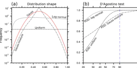
The POD is estimated for three non-Gaussian distribu-tions: uniform, log-normal, and a Gaussian mixture. The Gaussian mixture is defined through its PDF as P (x)=
w1P1(x)+w2P2(x)+w3P3(x)withP1,P2, andP3, three
Gaussian distributions with zero mean and respectively 0.1, 0.05, and 0.02 as chosen standard deviations. The chosen weights are given by(w1, w2, w3)=(0.2,0.5,0.3). The
rep-resentation of the shapes of these three distributions is given in Fig. 1a, alongside the Gaussian distribution.
PODs are estimated overNxp=105experiments. For both
tests, different ensemble sizesNsare tested (Ns=20, 30, 40,
Figure 1. (a) Three non-Gaussian distributions on which PODs
have been estimated: uniform distribution, log-normal distribution,
and Gaussian mixture (see text for description). (b) POD for K2
test. PODs are computed overNxp=105one-dimensional
experi-ments for different sample sizesNs.
the highest POD that reaches almost 1 as soon as the ensem-ble size is above 40. For the two others, the non-Gaussian distributions (uniform and Gaussian-mixture)K2test is only correctly discriminating from Gaussianity (with POD>0.8) when Ns>70. ForNs=90, which corresponds to the
en-semble size for the real data set composed of AROME-France forecasts (see Sect. 3), POD values are over 0.9 for all three non-Gaussian distributions. In conclusion, the K2 test is able to correctly discriminate NG for the ensemble size considered in this paper.
A review of other well-established tests for Gaussianity are presented in Bocquet et al. (2010), such as the measure of entropy (kullback (1959), used in geophysics by Pires et al. (2010)), or the univariate Anderson–Darling goodness-of-fit test (Anderson and Darling, 1954). The latter has been also tested in the same framework and the performances proved to be very similar to the ones of theK2test. When comparing the results, obtained over the ensemble (Sect. 3), these two tests also give very similar results; e.g. they indicate the same areas of NG over≈90 % of the domain. However, measuring skewness and kurtosis may be more informative and may be of interest for some assimilation schemes that account for skewness (Hodyss, 2012). Also, describing the values ofK2 has the advantage of preventing the results from depending on the chosen confidence level.
3 Diagnosis of the non-Gaussianity of AROME forecast errors
3.1 An AROME-France ensemble for a high-precipitating case
AROME-France is an operational nonhydrostatic model cov-ering France with a 2.5 km horizontal resolution at the time of the experiments. Its lateral boundary conditions are given
by the global model ARPEGE2. Assimilation steps are done every 3 h with a 3D-Var scheme and make use of a compre-hensive set of observations such as conventional, satellite or Doppler radar data (see Seity et al. (2011) for more details).
The simulation of background and analysis errors is achieved by using a Monte Carlo sampling, called an ensem-ble data assimilation (EDA) in the context of NWP. A 90-member EDA is first run for the global model (AEARP, Berre and Desroziers, 2010). Each EDA member is based on a 4D-Var cycled assimilation which uses perturbed observations and a perturbed background, in order to simulate the error evolution (Berre et al., 2006). Observation perturbations are constructed as random draws of the specified observation er-ror covariance matrix, and background perturbations result from the forecast evolution of previous analysis perturbations and from their inflation at the end of each forecast (Ray-naud et al., 2012). This global ensemble provides perturbed boundary conditions to an ensemble of perturbed 3D-Vars for AROME-France, as described in Ménétrier et al. (2014). True background errors are then approximated by the devia-tions of the perturbed backgrounds from the ensemble mean. A few cycles (typically four) are necessary to reach a regime where the spread of the ensemble is representative of the true error spread; these cycles are discarded from the diagnostics presented below.
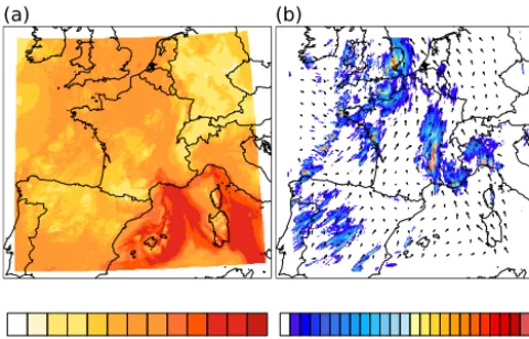
The case of interest is 4 November 2011 between 00:00 and 06:00 UTC (universal time coordinated). A strong southerly convergent flow occurs at low levels over southern France (Fig. 2). Warm and moist air from the Mediterranean sea is advected over land, which triggers deep convection. Those high intensity events, named cévenol events, are stud-ied by the HyMeX research program (Ducrocq et al., 2014). Associated precipitations are visible all along the Rhone Val-ley, with local maxima exceeding 25 mm h−1. Also, associ-ated with a low pressure area over the north-east Atlantic (not shown), a cold active front extending from the bay of Biscay to the eastern British coast is sweeping north-west of France with locally strong precipitations.
3.2 Vertical profiles of NG
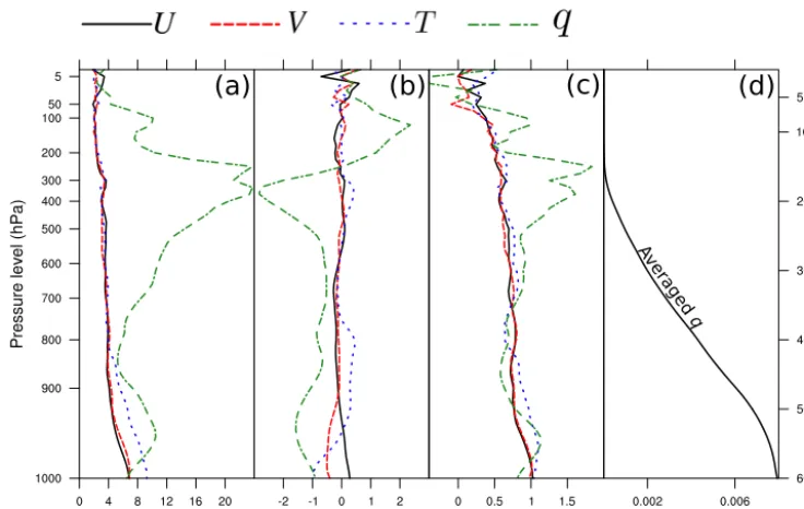
The vertical profiles of quantities related to NG are shown in Fig. 3 for 3 h forecasts of different variables, namely zonal (U) and meridian (V) winds, temperature (T) and specific humidity (q). On average, except near the surface,q is the variable that shows the largest deviation from Gaussianity, confirming results obtained at the global scale (Holm et al., 2002). From 850 to 350 hPa,q is indeed characterized with an increase of the deviation from Gaussianity. As shown in Fig. 3b, this NG is partly explained by negative values of the skewness, highlighting a left-tailed PDF of the background
2Action de Recherche Petite Échelle Grande Échelle (Pailleux
(a) (b)
Figure 2. (a) Specific humidity (q, kg kg−1) and (b) surface
cu-mulative precipitation (mm h−1) overlaid with winds vector at
model level 52 (≈920 hPa). Maps are given for one member of the
AROME-France 3 h forecasts ensemble, valid at 03:00 UTC on 4 November 2011.
errors, meaning that many values are more humid than the ensemble mean.
In the troposphere,K2is increasing while theqmean con-tent, displayed in Fig. 3d, is largely decreasing. Values at higher levels, where q is almost nonexistent, may however be taken with caution. Below 850 hPa,K2is peaking around 960 hPa. Above 850 hPa, the wind components andT remain close to Gaussianity. Below, however, all variables have sig-nificant deviation from Gaussianity, especiallyT for which high values ofK2are found at ground level, making of it the less Gaussian variable in the boundary layer.
3.3 Horizontal structures of NG
The range, defined as the difference between the 95th and the 5th percentiles, could be used to describe roughly the hori-zontal spatial variability for each vertical level. Vertical pro-files of ranges ofK2,f3(G3), andf4(G4)(not shown) have
large similarities between each other and with the shapes of K2 profiles displayed in Fig. 3a. They include in particu-lar two maxima in the boundary layer and in the high tro-posphere for q and larger values towards the surface for T. Ranges are much larger for the four variables (approximately four times as large) than the respective mean values given in Fig. 3, implying a large spatial variability for the three NG di-agnostics. An example of the horizontal structures of NG is given forqin the boundary layer by Fig. 4. They have large similarities with the meteorological coherent structures, as the southerly convergent flow over the south of France and the active cold front aloft the north-west of France are asso-ciated with high values ofK2.
Supporting the conclusion drawn from Fig. 3, transformed skewnessf3(G3)is mainly negative (corresponding to
left-tailed distributions) over the domain and has a larger contri-bution than transformed kurtosisf4(G4)in largeK2values.
Over the Mediterranean Sea, the skewness represents on av-erage 70 % ofK2.
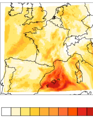
It may be interesting to compare NG with the variance of the ensemble, asK2 is defined from standard third and fourth standardized moments avoiding any scale effect. As displayed in Fig. 5, the variance does not coincide with over-all NG, even if it happens that Gaussian areas may coincide with regions of low variance.
NG of the surface pressure is not shown in this study since, according to our diagnostics, it is a mainly Gaussian variable (averagedK2around 2.7). High values ofK2appear around the cold front and the convergence area but they are very localized and of smaller amplitude compared to the other model variables.
3.4 Time evolution of non-Gaussianity
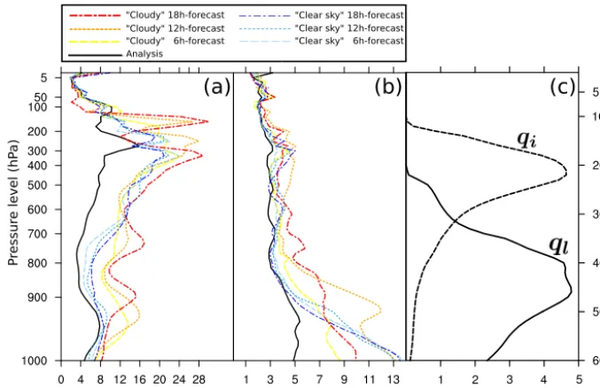
For each member of the ensemble, 18 h forecasts have been run from the analyses performed at 00:00 UTC on 4 Novem-ber 2011. This allows diagnosing NG every 6 h during the first 18 h of integration. The corresponding vertical profiles are shown in Fig. 6 for the two most non-Gaussian variables according to Sect. 3.2:q andT.
In order to get insights into the processes that may be in-volved in NG development, the diagnostics have been sepa-rately computed for cloudy and for clear sky areas, following a similar approach to that of Montmerle and Berre (2010) and Michel et al. (2011), in which precipitating masks have been used. Grid points over the domain are separated in two bins: “cloudy” or “clear-sky” points. The cloudy bin defines grid points whose vertically integrated simulated cloud wa-ter exceeds 0.1 g kg−1 for a majority of ensemble members (i.e. more than 45 members for the 90-member ensemble). The other points are classified as clear sky. The percentage of clear-sky points being 3–5 times larger (not shown) than the detected cloudy points, similarities between clear-sky pro-files, and profiles averaged over the whole domain (as plotted in Fig. 3) are apparent.
During the first 6 h of forecasts, NG quickly increases. For q, all tropospheric model levels are affected. ForT, starting from a fairly Gaussian profile, increase of NG is mainly af-fecting the boundary layer and higher levels remain close to Gaussianity. During the following 12 h (from 6 to 18 h fore-cast), changes of NG are smaller for both variables. Those results support that NG in the background may rather come from nonlinear processes acting on nearly Gaussian PDFs in-stead of linear processes acting non-Gaussian PDFs.
Model level Averaged
q
K2 f3(G3)
(a)
(b)
(c)
(d)
f4(G4)
Figure 3. Vertical profiles of (a)K2, (b) transformed skewnessf3(G3), (c) transformed kurtosisf4(G4), and (d)q(kg kg−1) for one member
of the ensemble. For each level, values are averaged over the horizontal domain. Profiles are computed from the 90-member ensemble of
AROME-France 3 h forecasts valid at 03:00 UTC on 4 November 2011. Profiles in (a), (b), and (c) are given for four model variables:U,V,
T, andq.
f3(G3) f4(G4)
K2
(a) (b) (c)
10 15 20 25 30 35 40 45 50 -11 -9 -7 -5 -3 -1 1 3 5 7 9 11 -11 -9 -7 -5 -3 -1 1 3 5 7 9 11
Figure 4. (a)K2, (b) transformed skewnessf3(G3), and (c) transformed kurtosisf4(G4)forqat model level 52 (≈920 hPa), computed
from the 90-member ensemble of AROME-France 3 h-forecast valid at 03:00 UTC on 4 November 2011.
is likely due to nonlinear processes such as the vertical dis-placement error of cloud base and top within the ensemble and possibly the diabatic processes. In surface layers, K2 for T quickly increases especially for clear air areas where turbulent and radiative processes occur. After 12 h, NG is more spread vertically within clouds, probably because of diabatic processes. ForT andq, diabatic processes are good candidates to produce NG because of intrinsic thresholds in cloud physics (e.g. moisture saturation) and nonlinear pro-cesses like turbulence on cloud-top.
For the wind components, behaviours close toT have been found but with smaller amplitude (not shown): NG increases mainly in the boundary layer in clear-sky areas and may be due to nonlinear turbulent processes.
Figure 5. Background-error standard deviations ofq(g kg−1) for
the model AROME-France, at model level 52 (≈920 hPa).
Stan-dard deviations are estimated from the 90-member ensemble of 3 h forecasts, valid at 03:00 UTC on 4 November 2011.
variables. The link between assimilated observations and NG reduction will be shown.
4.1 Overview
An overview of the NG evolution during the analysis process is given in Fig. 7 that shows averaged K2 profiles for the analysis and the background errors computed for two con-secutive assimilation/3 h forecast steps. Comparable results are found for the two cycles, confirming the increase of NG during the model integration and highlighting the substan-tial reduction of NG during the assimilation process, espe-cially for levels where NG grows quickly. Values ofK2are indeed brought back to much more Gaussian values, even in the lower levels for bothq andT and in the higher tropo-sphere forq.
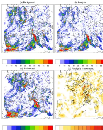
Geographical variations of NG are illustrated in Fig. 8. As in Fig. 7, the NG of the background and of the follow-ing 3 h forecast is similar. The largest decreases of NG be-tween background and analysis error match areas with a large analysis increment, in particular where radar data are assim-ilated (Fig. 8d). The analysis increment being a linear func-tion of the innovafunc-tion vector in model space (observafunc-tion mi-nus background), its Gaussianity is insured by a rough se-lection applied beforehand to the observations, allowing us to remove outliers (e.g. for radar data, Caumont et al., 2010; Wattrelot et al., 2014). Some NG areas remain though, espe-cially in areas where the background is less constrained by observations (e.g. above Spain and above the sea). However, most areas where NG has been reduced thanks to the data as-similation process recover their NG nature after 3 h of model integration.
4.2 Non-Gaussianity in control space
Previous results are documenting the NG of four model prognostic variables: U, V,T, and q. As it is detailed in Brousseau et al. (2011), the assimilation scheme in AROME-France is based on a 3D-Var whose control variables are the vorticity ζ, the unbalanced divergence ηu, the
unbal-anced temperature and surface pressure(T , Ps)u, and the
un-balanced specific humidityqu. These control variables are
linked to the model variables following the multivariate for-malism of Berre (2000), which is based on the decomposition of the background error covariance matrix in spatial opera-tors and balance transforms. Since the minimization is per-formed in the control space, NG diagnostics have also been computed for these control variables.
4.2.1 Overview
Vertical profiles of NG for control variables are presented in Fig. 9. Unlike the zonal and meridian winds,ζ andηu are
strongly non-Gaussian over the whole troposphere, whereas Tuandqudisplay much more Gaussian profiles.
Negative values off3(G3)below 800 hPa forηu(Fig. 9b)
denote a larger spread of the distribution below the mean, probably due to the occurrence of low level convergence. At mid-troposphere, error distributions of all four variables are near symmetric. Except for qu, distributions in
tropo-spheric levels remain symmetric and theK2index is mainly explained by the kurtosis (Fig. 9c).
Those results agree with one of the conclusions of Ménétrier et al. (2015). These authors describe an algorithm to find the optimal truncation dedicated to sample covari-ances filtering. This algorithm has two variants. The first one assumes a Gaussian PDF for the background perturbations while the second one does not. Their study indicates that, at convective scale, the Gaussian variant is accurate forTu
andqu, but the more general non-Gaussian variant has to be
used forζ andηu, which are significantly non-Gaussian
vari-ables in agreement with our study. To go further on this topic, NG diagnostics have been computed for the spatial first-order derivative ofT. WhileT is in average a locally nearly Gaus-sian variable (see Fig. 3a), its spatial differentiation largely increases the NG (not shown), up to the order of magnitude found in Figs. 9a and 10 forζ andη. This supports the attri-bution to differentiation for at least a part of the NG displayed for the dynamical control variables.
While very similar, the horizontal structures ofK2for ζ andηuare noisier compared to the other variables, with very
small scale and intense signals (not shown). Maps mostly fol-low the land–sea mask, with high values ofK2over sea and low values over land. Aloft, NG follows meteorological ac-tive structures (cold front and cévenol event).
P
ressur
e level (hP
a)
Model level
(a)
(b)
cloudy" ech 18h "cloudy" ech 12h
cloudy" ech 06hSC ear sky" ech 12h "clear sky" ech 18h
"clear sky" ech 06h
"Cloudy" 18h-forecast "Cloudy" 12h-forecast "Cloudy" 6h-forecast
Analysis
"Clear sky" 6h-forecast "Clear sky" 12h-forecast "Clear sky" 18h-forecast
(c)
K2 K2
Figure 6. Time evolution of the vertical profiles ofK2for (a)qand (b)T computed for (thick and hot colours) cloudy and (thin and cold colours) clear-sky points (see text). (c) Vertical profiles of liquid cloudql(solid line) and ice cloudqi(dashed line) contents (g kg−1). The
cloud contents are averaged over the domain and over times from 06:00 to 18:00 UTC, every 6 h. Initial cloud water profile is null because
the hydrometeors are not cycled. Consequently the initial time profiles ofK2are common for the two bins. Profiles have been computed
from 00:00 to 18:00 UTC, every 6 h, using forecasts initialized with analysis states valid on 4 November 2011, 00:00 UTC.
P
ressur
e level (hP
a)
Model level
(a) (b)
K2 K2
Run 00UTC: 3h-forecast
Run 00UTC: analysis RRunun 03UTC: 3h-forecast 03UTC: analysis
Figure 7. Vertical profiles of K2on background and analysis
er-rors for (a)qand (b)T, for two successive cycled assimilation/3 h
forecast steps starting at 00:00 UTC on 4 November 2011.
900 hPa are almost unchanged, the averaged K2ofζ andη is systematically lower for the analysis than the background state in the boundary layer. However, the order of magnitude of the decrease is much smaller than for T andq, and the dynamical variablesζ andηremain by far much more non-Gaussian.
4.2.2 Non-Gaussianity in the multivariate transform To go further in the discussion on Gaussianity of the control variables, this section compares theK2values for total and unbalanced variables.
According to Fig. 10, the debalancing process is not really affecting the NG for the divergence, except at lower levels whereK2is slightly decreasing while keeping large values. K2values remain 2–3 times larger for the divergence (total or unbalanced) than forT andq from the surface to the mid-troposphere. On the contrary, NG decreases significantly for T andqduring the debalancing process. Changes mainly ap-pear in the boundary layer forT. Forq, changes appear for every model level, especially in the boundary layer and be-low the tropopause. From the surface to 750 hPa, the NG of quis equal to or smaller than the NG ofTu.
5 Conclusions
Figure 8.K2forqat level 52 (≈920 hPa) for (a) the background, (b) the analysis, and (c) the following 3 h forecast starting at 03:00 UTC
on 4 November 2011. (d) Corresponding analysis increment (kg kg−1) with positions of radar precipitation observations assimilated.
behaviours for a case study characterized by a cévenol event and an active cold front.
According to our diagnostic, among model variables,qhas the largest deviation from Gaussianity, with a maximum of amplitude near the tropopause and in the boundary layer. De-viation from Gaussianity forU,V, andT only appears in the boundary layer. With an heterogeneous diagnostic, NG has been separately diagnosed for cloudy points and clear-sky points. Forq, cloud covering leads to higher NG, especially at the bottom and at the top of the cloud layer. In clear-sky situations, surface processes are expected to enlarge K2for T, in a larger manner than for cloudy points. Studying time evolution through forecast ranges, NG is mainly increasing during the first 6 h. The 3D-Var assimilation appears to
effi-ciently reduce the growing NG of the forecast, especially in well-observed areas. Finally, among control variables of the assimilation,ζ andηudeviate from Gaussianity in a larger
manner thanTuandqu, which are much more Gaussian than
their balanced counterparts.
Model level
f3(G3)
K2 f
4(G4)
(a)
(b)
(c)
Figure 9. Vertical profiles of (a)K2, (b) transformed skewnessf3(G3), and (c) transformed kurtosisf4(G4). For each level, values are
aver-aged over the horizontal domain. Profiles are computed from the 90-member ensemble of AROME-France 3 h forecasts valid at 03:00 UTC on 4 November 2011. Profiles in (a), (b), and (c) are given for four control variables:ζ,ηu,Tu, andqu.
P
ressur
e level (hP
a)
Model level
Figure 10. Comparison ofK2vertical profiles of model variables (thick lines) and control variables (thin lines). Profiles are computed from 3 h forecasts valid at 03:00 UTC on 4 November 2011.
2002), but the discussion may also be focused on vorticity and divergence, either with a Gaussianization of those vari-ables or with a discussion on the possibility to use other dy-namical variables. Second, with the cloud mask approach, cloud layers have been associated with high values of NG.
This study uses an ensemble at convective scale that does not include model error either in the analysis or in the fore-cast steps. It is possible that conclusions would be different if stochastic noise drawn explicitly from a Gaussian distri-bution is added to the model states during the forecasts, as stated by Lawson and Hansen (2004). Also, this study is ac-tually a part of work focused on the correction of displace-ment errors. Since displacedisplace-ment errors are identified to cause NG (Lawson and Hansen, 2005), diagnostics of NG may be used to evaluate improvements in the current amplitude er-ror correction step (3D-Var) brought by a displacement erer-ror correction (Ravela et al., 2007). This will be examined in fu-ture work.
Acknowledgements. This work has been supported by the French Agence Nationale de la Recherche (ANR) via the IODA-MED Grant ANR-11-BS56-0005 and by the MISTRALS/HyMeX pro-gram. The authors thank Benjamin Ménétrier, Gérald Desroziers, and Loïk Berre for their scientific advice and their careful readings that proved very useful to improve the manuscript.
Edited by: O. Talagrand
Reviewed by: C. Pires and two anonymous referees
References
Anderson, E. and Järvinen, H.: Variational quality
control, Q. J. Roy. Meteorol. Soc., 125, 697–722,
doi:10.1002/qj.49712555416, 1999.
Anscombe, Francis J. and Glynn, William J.: Distribution of the kurtosis statistic b2 for normal samples, Biometrika, 70, 227– 234, 1983.
Auligné, T., Lorenc, A., Michel, Y., Montmerle, T., Jones, A., Hu, M., and Dudhia, J.: Toward a new cloud analysis and prediction system, B. Am. Meteorol. Soc., 92, 207–210, 2011.
Berre, L.: Estimation of synoptic and mesoscale forecast error co-variances in a limited-area model, Mon. Weather Rev., 128, 644– 667, 2000.
Berre, L. and Desroziers, G.: Filtering of background error vari-ances and correlations by local spatial averaging: a review, Mon. Weather Rev., 138, 3693–3720, 2010.
Berre, L., Ecaterina ¸Stef˘anescu, S., and Belo Pereira, M.: The rep-resentation of the analysis effect in three error simulation tech-niques, Tellus A, 58, 196–209, 2006.
Bocquet, M., Pires, C. A., and Wu, L.: Beyond Gaussian statistical modeling in geophysical data assimilation, Mon. Weather Rev., 138, 2997–3023, 2010.
Brousseau, P., Berre, L., Bouttier, F., and Desroziers, G.: Background-error covariances for a convective-scale data-assimilation system: AROME–France 3D-Var, Q. J. Roy. Mete-orol. Soc., 137, 409–422, 2011.
Caumont O., Ducrocq V., Wattrelot E., Jaubert G., and PRADIER-VABRE S.: 1D+ 3DVar assimilation of radar reflectivity data: A proof of concept, Tellus A, 62, 173–187, 2010.
Courtier, P., Thépaut, J.-N., and Hollingsworth, A.: A strategy for operational implementation of 4D-Var, using an incremental ap-proach, Q. J. Roy. Meteorol. Soc., 120, 1367–1387, 1994. D’Agostino, R. B.: Transformation to normality of the null
distri-bution of G1, Biometrika, 57, 679–681, 1970.
D’Agostino, R. B., Belanger, A., and D’Agostino Jr, R. B.: A sug-gestion for using powerful and informative tests of normality, Am. Stat., 44, 316–321, 1990.
Dee, D. P. and da Silva, A. M.: The choice of variable for atmo-spheric moisture analysis, Mon. Weather Rev., 131, 155–171, 2003.
Ducrocq, V., Belamari, S., Boudevillain, B., Bousquet, O., Coc-querez, P., Doerenbecher, A., Drobinski, P., Flamant, C., Labatut, L., Lambert, D., Nuret, M., Richard, E., Roussot, O., Testor, P., Arbogast, P., Ayral, P.-A., Van Baelen, J., Basdevant, C., Boichard, J.-L., Bourras, D., Bouvier, C., Bouin, M.-N., Bock, O., Braud,I., Champollion, C., Coppola, L., Coquillat, S., De-fer, E., Delanoë, J., Delrieu, G., Didon-Lescot, J.-F., Durand, P., Estournel, C., Fourrié, N., Garrouste, O., Giordani, H., Le Coz, J., Michel, Y., Nuissier, O., Roberts, G., Saïd, F., Schwarzen-boeck, A., Sellegri, K., Taupier-Letage, I., and Vandervaere J.-P.: HyMeX, les campagnes de mesures: focus sur les événements extrêmes en Méditerranée, Société météorologique de France, Paris, France, La Météorologie, 80, 37–47, 2013.
Ducrocq, V., Braud, I., Davolio, S., Ferretti, R., Flamant, C., Jansá, A., Kalthoff, N., Richard, E., Taupier-Letage, I., Ayral, P.-A., Belamari, S., Berne, A., Borga, M., Boudevillain, B., Bock, O., Boichard, J.-L., Bouin, M.-N., Bousquet, O., Bouvier, C., Chig-giato, J., Cimini, D., Corsmeier, U., Coppola, L., Cocquerez, P., Defer, E., Delanoë, J., Di Girolamo, P., Doerenbecher, A., Drobinski, P., Dufournet, Y., Fourrié, N., Gourley, J. J., Labatut, L., Lambert, D., Le Coz, J., Marzano, F. S., Molinié, G., Mon-tani, A., Nord, G., Nuret, M., Ramage, K., Rison, B., Roussot, O., Said, F., Schwarzenboeck, A., Testor, P., Van-Baelen, J.,
Vincen-don, B., Aran, M., and Tamayo, J.: HyMeX-SOP1, the field cam-paign dedicated to heavy precipitation and flash flooding in the northwestern Mediterranean, B. Am. Meteorol, Soc., 95, 1083– 1100, doi:10.1175/BAMS-D-12-00244.1, 2014.
Fisher, M.: Background error covariance modelling, in: Seminar on Recent Development in Data Assimilation for Atmosphere and Ocean, ECMWF, 45–63, 2003.
Gustafsson, N., Thorsteinsson, S., Stengel, M., and Holm, E.: Use of a nonlinear pseudo-relative humidity variable in a multivariate formulation of moisture analysis, Q. J. Roy. Meteorol. Soc., 137, 1004–1018, doi:10.1002/qj.813, 2011.
Hodyss, D.: Accounting for skewness in ensemble data assimila-tion, Mon. Weather Rev., 140, 2346–2358, 2012.
Holm, E., Andersson, E., Beljaars, A., Lopez, P., Mahfouf, J.-F., Simmons, A., and Thépaut, J.-N.: Assimilation and modelling of the hydrological cycle: ECMWF’s status and plans, European Centre for Medium-Range Weather Forecasts (ECMWF), Tech-nical Memorandum, 2002.
Houtekamer, P., Lefaivre, L., Derome, J., Ritchie, H., and Mitchell, H. L.: A system simulation approach to ensemble prediction, Mon. Weather Rev., 124, 1225–1242, 1996.
Ingleby, N., Lorenc, A., Ngan, K., Rawlins, F., and Jackson, D.: Improved variational analyses using a nonlinear humidity control variable, Q. J. Roy. Meteorol. Soc., 139, 1875–1887, 2013. Kalnay, E.: Atmospheric modeling, data assimilation, and
pre-dictability, Cambridge University Press, p. 341, 2003.
Kullback, S.: Information theory and statistics, New York, Wiley, 395 pp., 1959.
Laroche S. and Gauthier, P.: A validation of the incremental for-mulation of 4D variational data assimilation in a nonlinear barotropic flow, Tellus A, 50, 557–572, 1998.
Lawson, W. G. and Hansen, J. A.: Implications of stochastic and deterministic filters as ensemble-based data assimilation meth-ods in varying regimes of error growth, Mon. Weather Rev., 132, 1966–1981, 2004.
Lawson, W. G. and Hansen, J. A.: Alignment error models and ensemble-based data assimilation, Mon. Weather Rev., 133, 1687–1709, 2005.
Lorenc, A. C.: Analysis methods for numerical weather prediction, Q. J. Roy. Meteorol. Soc., 112, 1177–1194, 1986.
Ménétrier, B., Montmerle, T., Berre, L., and Michel, Y.: Estimation and diagnosis of heterogeneous flow-dependent background-error covariances at the convective scale using either large or small ensembles, Q. J. Roy. Meteorol. Soc., 140, 2050–2061, 2014.
Ménétrier, B., Montmerle, T., Michel, Y., and Berre, L.: Linear fil-tering of sample covariances for ensemble-based data assimila-tion, Part I: optimality criteria and application to variance filter-ing and covariance localization, Mon. Weather Rev., 143, 1622– 1643, 2015.
Michel, Y., Auligné, T., and Montmerle, T.: Heterogeneous convective-scale background error covariances with the inclusion of hydrometeor variables, Mon. Weather Rev., 139, 2994–3015, 2011.
Pailleux, J., Geleyn, J.-F., and Legrand, E.: La prévision numérique du temps avec les modèles ARPÈGE et ALADIN-Bilan et per-spectives, La Météorologie, 2000.
Pires, C. A., Talagrand, O. and Bocquet, M.: Diagnosis and impacts of non-Gaussianity of innovations in data assimilation, Phys. D, 239, 1701–1717, 2010.
Rabier, F., Järvinen, H., Klinker, E., Mahfouf, J.-F., and Sim-mons, A.: The ECMWF operational implementation of four-dimensional variational assimilation. I: Experimental results with simplified physics, Q. J. Roy. Meteorol. Soc., 126, 1143–1170, 2000.
Ravela, S., Emanuel, K., and McLaughlin, D.: Data assimilation by field alignment, Phys. D, 230, 127–145, 2007.
Raynaud, L., Berre, L., and Desroziers, G.: Accounting for model error in the Météo-France ensemble data assimilation system, Q. J. Roy. Meteorol. Soc., 138, 249–262, 2012.
Seity, Y., Brousseau, P., Malardel, S., Hello, G., Bénard, P., Bouttier, F., Lac, C., and Masson, V.: The AROME-France convective-scale operational model, Mon. Weather Rev., 139, 976–991, 2011.
Tavolato, C. and Isaksen, L.: On the use of a Huber norm for obser-vation quality control in the ECMWF 4D-Var, Q. J. Roy. Meteo-rol. Soc., doi:10.1002/qj.2440, 2014.