On the randomness that generates biased samples: The
limited randomness approach
George Lagogiannis1, Stavros Kontopoulos2, and Christos Makris3 1 Department of Agricultural Economics and Rural Development,
Agricultural University of Athens, Iera odos 75, 11855, Athens, Greece
Department of Computer Engineering and Informatics, University of Patras, 26500 Patras, Greece
3 Department of Computer Engineering and Informatics, University of Patras,
26500 Patras, Greece [email protected]
Abstract. We introduce two new algorithms for creating an exponentially biased sample over a possibly infinite data stream. Such an algorithm exists in the literature and usesO(logn)random bits per stream element, wherenis the number of ele-ments in the sample. In this paper we present algorithms that useO(1)random bits per stream element. In essence, what we achieve is to be able to choose an element at random, out ofnelements, by sparingO(1)random bits. Although in general this is not possible, the exact problem we are studying makes it possible. The needed randomness for this task is provided through a random walk. To prove the correct-ness of our algorithms we use a model also introduced in this paper, thelimited randomnessmodel. It is based on the fact that survival probabilities are assigned to the stream elements before they start to arrive.
Keywords:Biased reservoir sampling, Markov chain, random walk.
1.
Introduction
Let us assume that we want to create a fixed size subset of a data stream of unknown, possibly infinite length. We call this subset asampleand letnbe the given size of the sample, dictated by the available for this purpose memory. Creating such a sample falls into the general category of synopsis maintenance([3], [6], [7], [10], [12], [14], [16], [17]). The problem of synopsis maintenance has been studied extensively for estimating queries ([4], [7], [17]) in data streams. A survey of stream synopsis construction algo-rithms can be found in [2].
stream progresses (see [16]). This means that as the stream progresses, fewer and fewer elements in the sample belong to the recent history of the stream. Such a sample may be proved useless for answering queries concerning the recent past. To address this problem one needs to create a biased sample. Such a sample is created in [1].
In [1], a bias functionf(r, t)is associated with ther−thstream element at the time of arrival of thet −th stream element(r ≤ t). This function is associated with the probabilityp(r, t)of ther−thelement belonging to the sample at the time of thet−th
element. In particular, the functionf(r, t)is monotonically decreasing witht(for fixedr) and monotonically increasing withr(for fixedt). For the specific functione−λ(t−r), an efficient algorithm is introduced in [1] for creating a sample consistent with that function. The parameterλdefines the bias rate and typically lies in the range [0, 1]. In general,
λis chosen in an application–specific way and it is the inverse of the number of stream elements after which the relative probability of inclusion in the sample reduces by a factor of1/e. Throughout this paper, we name this algorithmAlgorithm A. Also, we assume that
f(r, t)is identical top(r, t).
The introduction of bias results in some upper bounds on the maximum necessary sample size, also calledmaximum reservoir requirement. It is proved in [1] that for the exponential bias function, the maximum reservoir requirement is bounded above by1/λ, assuming thatλis much smaller than 1, which happens to be the most interesting case. According to AlgorithmA, each new stream element takes the place of another element of the sample which is chosen uniformly at random. Given that the size of the sample is
n, Algorithm A needsO(logn)random bits per stream element, in order to choose an element of the sample at random.
In this paper we are going to present algorithms for creating a biased reservoir sample (over a very long, possibly infinite stream of data) consistent with the exponential bias function. The algorithms are based on the unit-cost RAM model, and useO(1)random bits per stream element in the worst-case. Thus, our algorithms outperform Algorithm A in terms ofrandomness complexity.
The issue of reducing the randomness complexity of algorithms is not only of theo-retical interest, but of practical as well. The analysis of randomized algorithms is always based on some assumptions concerning the theoretical machine-model used. The most frequently used machine-model is the unit-cost RAM. An interesting assumption con-cerning the unit-cost RAM, is that it needsO(1)time to uniformly choose an element at random overnelements. This is becauseO(logn)random bits are needed for this task and the unit-cost RAM accesses these bits in O(1) time (we assume thatw, the word size, is bigger thanlogn). However this is not realistic, because the actual cost of generating these bits is swept under the carpet, through its assignment to some subroutine that has no cost at all. All the unit-cost RAM needs to do, is to spendO(1)time in order to access
complexity isO(logn) (all the time complexities are “per stream element”). Assuming that each random bit costsO(1)time (following the logic of [8]), the random bits in Al-gorithm A introduce a multiplicative factor ofO(logn)per stream element in the time complexity. Our algorithms avoid this multiplicative factor and the intuition behind this result is given in the following paragraphs.
Let us assume that we have a coin, claimed to be fair. Intuitively, this means that if we toss the coin M times, “heads” or “tails” is supposed to occur at a fraction of M
that approaches 1/2, as M approaches infinity. However, to evaluate the coin (i.e. to decide whether the coin is fair or not) we do not need to toss the coin M times, for a big enoughM. It suffices to inspect its shape (assume that we have special equipment for this). Clearly, the time of such an inspection is irrelevant (assuming that the shape of the coin remains unchanged over time). Let us now follow the same logic, replacing the coin by an algorithm that creates a sample over a data stream. The coin produces “heads” or “tails”, whereas the algorithm produces samples. By setting the sample to be consistent with a bias functionp(r, t), we mean that if we execute the algorithmM times on a streamS, ther−thstream element (i.e.,S(r)) will survive in the sample at timet
(t > r)at a fraction of theM produced samples that approachesp(r, t)asMapproaches infinity. In order to evaluate such an algorithm (i.e. to decide whether or not the algorithm creates a sample consistent withp(r, t)), we need to check its instructions and using these instructions to calculate survival probabilities for the sample elements. If these survival probabilities are consistent with the given bias function, we conclude that the algorithm works as claimed. As with the coin, the time of the evaluation is irrelevant (clearly, the algorithm remains unchanged over time). Although the evaluation can be performed any time, the evaluation at timet = 0(i.e. before the stream elements start to arrive) has a clear advantage, to be explained in the following paragraphs. Evaluating the algorithm at timet = 0, means that we have no sample to inspect but we do not actually need an existing sample. It is the “shape of the coin” that matters.
In order to successfully evaluate our algorithms, we must conclude that each time a new stream element arrives, each sample element is equally likely to be deleted from the sample (this is the basic property of the sampling algorithm in [1]). This means that each time a new stream element arrives, we need to perform uniform sampling. For this pur-pose, our algorithms use a Markov chain whose stationary distribution happens to be the uniform distribution. The random walk corresponding to this Markov chain is composed ofsteps. Each time, one of the elements of the sample is thepositionof the walk. Each step results in a new position of the walk and needsO(1)random bits in the worst-case. Each accessed random bit is used for executing a step of the walk and we choose to delete the element of the sample implied by the position of the walk.
The above claim may sound strange. In particular, one may argue that when an element is chosen by our algorithm at any timet6= 0, the position of the walk is deterministically decided. Knowing the position of the walk at timet, how is it possible to choose the next element uniformly at random, by accessing onlyO(1)random bits? The answer is the following: Accessing the sample at timet 6= 0and calculating survival probabilities for the sample elements, we simply calculate conditional probabilities in regard to timet= 0, i.e. probabilities under the condition that the exact accessed sample of timetwill occur. In this sense, calculating survival probabilities at any timet6= 0, may be misleading.
To achieve uniform sampling while calculating survival probabilities at timet= 0, it suffices to make sure that by the time the stream elements start to arrive, the Markov chain will have reached its stationary distribution (i.e., the uniform distribution). As a result, it will remain in this distribution, which means that in regard to time t = 0, all future elements are equally likely to be chosen by our algorithm. More insight on this claim will be given in Section 3, where a more detailed intuitive example is given. We will also use the example of Section 3 for intuitively introducing a new model for evaluating our algorithms, which we calllimited randomnessmodel.
The structure of the paper is the following: In Section 2, we briefly present Algorithm A. In Section 3 we present the intuition behind the definitions that we present in Section 4. In Section 5, we present the random walk. This way we use this random walk as a black box in Section 6, where we present our new algorithms. We believe that this “black box” usage of the random walk simplifies the description of the algorithms, and helps the reader focus on the rest of the ideas that make our algorithms work.
2.
Algorithm A: The exponential bias function
In this section, we will briefly present AlgorithmA(i.e., algorithm 2.1 of [1]).
Algorithm A is based on the idea that each new stream element is deterministically inserted into the sample, and replaces one of the old elements of the sample. The old ele-ment to be replaced is chosen uniformly at random. Therefore, assuming that the reservoir containsnelements, each element “survives” in the sample with probability(1−1/n)
every time a new stream element arrives. Then, the element that arrives at timerwill exist in the sample at timetwith probability(1−1/n)t−r = ((1−1/n)n)(t−r)/n. For large values ofn(and it is reasonable to assume thatnis large), the inner(1−1/n)nterm is approximately equal to1/e, and from substitution, the exponential bias function follows. It must be noted that AlgorithmAis slightly more complicated, because the reservoir is filled gradually, to ensure that the sample is consistent with the exponential bias function from the beginning. We have skipped this part, firstly in order to keep things simple, and secondly because we are going to use the exact methodology, to achieve the same thing.
3.
Intuition on the term “limited randomness ”
We can use a roulette as an intuitive example. Let us assume that we have a roulette with
distant ones, to host the ball after the next “throw”. This weakness of our roulette comes from the fact that the ball is moved by means of a random walk algorithm (it is an e-roulette). The random walk uses less randomness than what is actually needed in order to guarantee that each time, the ball ends up in a slot that can be assumed to be fully random (it is therefore alimited randomness roulette). Although in the long run, one will observe that each number is equally likely to occur, the casino owners have a problem. If the players know the algorithm under which the roulette operates, they will bet their money on slots nearby the most recent winning slot. Even if the players do not know the algorithm under which the roulette operates, they can observe and notice that each time, the ball tends to end-up in a slot that is nearby the previous one. If the casino owners use this roulette in the “traditional” way, their casino is doomed.
To address the issue, the casino owners apply a curtain above the roulette, so that the players cannot see where the ball is before the throw. If the casino owners manage to hide all the information concerning the current position of the ball, so that the players conclude that below the curtain, the ball is equally likely to be in any slot, the problem is solved. This curtain is the basic notion of our mechanism and it will be modeled in the next section. The players now havelimited accesson what is going on.
One might wonder how is it possible to use this roulette instead of the traditional one. In particular, it is clear after a throw, the winning number must be revealed to the players and then the players will bet their money on nearby slots. Even if they cannot see the slots (i.e. they do not know which number corresponds to each slot), they will write down the winning numbers. Each time a winning numberxappears, they will check their notes and see what is the most frequent winning number next ofx. Then, they will bet their money on this number. It seems that the notion of the curtain did not make this roulette usable after all. Clearly, assuming that the players have no memory of the past, the problem is solved. But is such an assumption reasonable? For casino players, it certainly isn’t.
However keep in mind that the central idea behind the algorithms presented in this paper, is that all evaluations (i.e., all probability calculations) are performed at timet= 0
(according to the intuition given in Section 1). Assuming that the players have no memory of the past, we simply incorporate into our model the fact that at timet = 0, when the evaluation occurs, there is nothing to remember. Thus, our limited randomness roulette can in fact be used, but not with a curtain (the curtain only exists in our evaluation model). The exact use is presented in the next paragraph.
4.
Definitions
In general, we distinguish in this paper two approaches for a biased reservoir sampling algorithm: According to the strictapproach, the reservoir is filled gradually and even when it is not full, the sample is consistent with the bias function. According to thegreedy
approach the reservoir is first filled and then the algorithm starts. Therefore it follows that initially, our sample does not comply with the bias function. But as time passes, fewer and fewer of the initial elements continue to exist in the sample, thus the fraction of the sample that was not built according to our function, continuously decreases. By the above definition, AlgorithmAis strict.
We distinguish the memory positions used by an algorithm that creates a biased sam-ple, into two parts. Thesample-space, contains all the memory positions where the el-ements of the sample are stored. Thesurrounding-spacecontains all the memory posi-tions used by the algorithm in order to obtain the sample, except the sample-space. The sample-space and the surrounding-space together, correspond to theentire used-spaceof the algorithm. Let us now introduce the concept of thesample-user, which informally, is a person able to calculate probabilities and comes in two flavors.
Definition 1. Thesample-user of full accessis anevaluatorable to access at any timet
i) the entire used-space, ii) the algorithm that created the sample and iii) the bias function associated with the algorithm. Based on what he/she can access at timet, the sample-user of full access is able to calculate for each existing or future sample-elementx, the probability ofxbeing in the sample for all future (in regard tox) time-points.
Definition 2. Thesample-user of limited accessis anevaluatorable to access at any timeti) the sample-space, ii) the algorithm that created the sample and iii) the bias func-tion associated with the algorithm. Based on what he/she can access at timet, the sample-user of limited access is able to calculate for each existing or future sample-elementx, the probability ofxbeing in the sample for all future (in regard tox) time-points.
It must be noted that in both definitions, we consider the sample-user to be memory-less, in the following sense: At any given timet, the sample-user of full (limited) access is able to calculate probabilities based on what he/she is able to access at time tonly. In other words, the sample-user can not keep track of the changes that have occurred to the sample, in order to use the information provided by these changes when calculating probabilities.
The notion of the sample-users is introduced in order to capture the intuition described in the previous section. The different flavors of a sample-user are needed to capture the presence or absence of a curtain that covers all memory positions except the sample-space. According to the above two definitions, the only time-point where a sample-user of full access and a sample-user of limited access have the same “power” is the time before the stream elements start to arrive (i.e., whent= 0). This is because at timet= 0, the entire used space is empty. We have set the sample-users to be memoryless in order to reflect to the sample-users the fact that all calculations are done at timet= 0because there is nothing to remember at timet= 0.
Definition 4. A biased sampleof limited randomness consistent with a function f
is a sample where at any time t, a sample-user of limited access is not able to find an existing or future elementxin the sample, for which at least one time-point decreases the probability ofxbeing in the sample in a way different than the one dictated byf.
Definition 3 applies to the biased sample created in [1]. In particular, at any timet, the sample-user of full access will conclude by accessing Algorithm A, that each of then
elements in the sample has1/nprobability of being deleted from the sample at the next time-point, i.e. each element has(1−1/n)probability to survive the next insertion, and this is consistent with the exponential bias function (allowing the substitutions explained in Section 2). Said otherwise, Algorithm Aconvincesa sample-user of full access.
In this paper we present algorithms for creating a biased sample of limited random-ness, i.e. algorithms that convince a sample-user of limited access. According to the intu-ition given so far, convincing a sample-user of limited access suffices for proving that our algorithms produce samples consistent with a given bias function. This is because time
t = 0is as good as any for evaluating our algorithms and it turns out that at timet = 0, a sample user of limited access and a sample user of full access are identical (they both access the same thing, i.e. the instructions of the algorithm). We believe that this limited access model can be used in order to reduce the randomness complexity of algorithms, in cases where the randomness complexity dominates the overall time complexity.
5.
The random walk
5.1. Description of the random walk
In this subsection we present an algorithm for performing a random walk on a list. The list is traversed in left-to-right order, with the leftmost node being the head of the list. Thus, the next node of a nodeuis the node on the right ofu, and we set the next node of the rightmost node of the list to be the head of the list (i.e., we actually have a circle). Similarly, the previous node ofuis the node on the left side ofu, and the previous node of the head of the list is the rightmost node of the list. We also maintain a pointer called
cursor, that points to a node of the list which we callposition of the walk. The walk consists of steps, with each step having an initial, and a final node. The initial node is the position of the walk before the step starts, and the final node is the position of the walk after the step ends. The previous of the final node is calledhit-node, and thus each step “produces” a hit-node. Initially, before the first step, the position of the walk is the head of the list. A step is briefly described by algorithm Step that follows.
Algorithm Step. We toss a fair coin on the position of the walk. If “tails” occur, the next node of the list becomes the position of the walk, and we repeat the same (i.e. we toss a fair coin again). Otherwise, the position of the walk becomes the hit-node of Step(), we set the cursor to point to the next node (which now becomes the position of the walk) and Step() ends. The maximum number of coins we are allowed to toss, is K. If we tossKcoins and no “heads” occur, then we declare the node pointed by the cur-sor as hit-node, we set the curcur-sor to point to the next node of the list and Step() ends.
value ofK, the maximum number of coin-tosses we are allowed to have in each step. Obviously, the worst-case time complexity of Step is equal toK. However, as long as
K ≥ 2, observe that since the coin is fair, 2 coin tosses are performed on the average in each step, because this is the average number of tosses until “heads” occur. Thus, the expected number of random bits per step is 2 and Step costsO(1) expected time. By allowingccoin tosses at most, wherecis a constant greater than one, we achieve constant worst-case time per step. By allowing only one coin toss, no randomness is inserted into the scheme, and the position of the cursor becomes deterministic for all the future time points.
5.2. Analysis of the random walk
Letnbe the length of the list. We will analyze the walk forKsuch that2≤K≤n. Let
mi= 1/2iand
pi=
mi, ifi < K
mi−1, ifi=K
0, ifi > K
We can easily see that the walk can be described by a Markov chain with the following
n∗ntransition matrix.
P =
pn p1p2p3. . . pn−1
pn−1pnp1p2. . . pn−2 ..
. ... ... . . . ...
p1 p2p3p4. . . pn
For example, by settingK=nthe matrix becomes:
P =
1/2n−1 1/2 1/4 1/8 . . .1/2n−1
1/2n−11/2n−11/2 1/4 . . .1/2n−2 ..
. ... . . . ...
1/2 1/4 1/8 1/16. . .1/2n−1
For more details and an extended example see Appendix A. The key observations are that the factors are the same for each row and their sum is equal to 1. The position probability vector at timejis:
P osj =
P1,jP2,j. . . Pn,j
and can be derived by the initial probability vector at time 0,θ=
P1,0P2,0. . . Pn,0
as follows:P osj =θ∗P(j−1).
Theorem 1 The random walk described in this subsection simulates a uniform sampling process as time approaches infinity.
probability of returning to a state is greater than 0, since we can reach any state from any other state with probability greater than 0. The above statements hold for any K. Thus the Markov chain has one limiting distributionπsuch thatπ∗P = πandPni=1πi = 1, whereπi>0. It is straightforward to see thatπ= [1/n,1/n,· · ·,1/n].
5.3. Mixing time of the random walk
Theorem 1 establishes the fact that after “a while”, the probability distribution of the Markov chain becomes very close to the uniform distribution. An important issue is how long it is going to take, i.e. what is the mixing time of the chain, defined as follows: Let V be the state space of our Markov chain. Let us assume that the chain will ulti-mately converge to the stationary distributionπ which means that for everyi, j ∈ V,
limt→∞(Pt)ij =πj. TheL2mixing timer() = maxx∈V min{t: ||ktx−1||2,π ≤} is the worst-case time for standard deviation of the densitykxt(y) = (Pt)xy
πy to drop to
[15]. For reasons of completeness we have calculated this mixing time in Appendix B and it isO(n2·logn)wherenis the number of list-nodes.
The mixing time is independent ofK. Thus, by increasingK, one expects that the chain will reach the stationary distribution faster, but not asymptotically faster. While asymptotically there is no gain in settingKto be high, there is a gain in settingKto be a constant: The number of random bits per stream element becomes constant in the worst case. This is why in the following of the paper, we setK= 2.
6.
New algorithms
LetS(r)be ther-th stream element. Each arriving stream element defines the current time, i.e. ther-th stream element arrives at time-pointr. Recall that in [1], it is proved that the reservoir size is bounded above by1/λ. As a result, initially, we have a list of1/λ
nodes, which we callsample-list. The sample-list is traversed in left-to-right order. The leftmost node is node 1, and the numbers of the nodes increment as we walk rightwards, however the numbers are only implied by the relative order of the nodes in the list and they are not stored in the nodes. The sample-list is the sample-space defined in Section 4. We are going to present two new algorithms for creating a sample consistent with the exponential bias function. More specifically, we are going to show that according to both algorithms, the probability of S(r)being in the sample at timet (for anyt ≥ r) ise−λ(t−r). In order to better state the problem we need to solve, we are going to first introduce a simple but problematic algorithm which we call Algorithm 0. In order to make things even simpler, let us assume that each sample element (stored in a node of the sample-list) is accompanied by its arrival time. That is, by accessing a node of the sample-list, we access an element of the sample, and the arrival time of this element.
Algorithm 0. When a new stream element arrives (after the reservoir is filled), we execute algorithm Step(), and replace the element stored in the hit-node by the new stream element.
Knowing the instructions of our algorithm and accessing the sample-list, the user is able to deterministically decide on the position of the walk: In particular, the cursor points to the next node of the node that contains the most recent element of the sample. This knowl-edge allows the user to determine for all the elements in the sample, a survival probability for the next time-point different than the one dictated by the exponential bias function. For example, the user will conclude that the element pointed by the cursor has 1/2 probability of being the next to be deleted. If the user starts calculating future probabilities, he/she will conclude that for any time-point more distant into the future thanr()time-points, each element can be assumed to be chosen uniformly at random and this is consistent with the given bias function. But for any future time-point betweentandt+r(), the user will conclude that the instructions of the algorithm do not comply with the given bias function. An issue that must be discussed, is whether Algorithm 0 manages to convince a sample-user of limited access, if we do not accompany each sample element by its ar-rival time. Then, the user cannot find the most recent element, therefore cannot decide on the position on the walk. However, this holds only for the elements that already exist in the sample, because the sample-user can obviously connect the future positions of the walk with the positions of the future elements. In particular, after the insertion ofS(t)for a future time-pointt, the cursor will point to the node next to the one that containsS(t). Therefore, assumingK = 2, the probability thatS(t)will be deleted at timet+ 1is 0 (we assume that the sample-list contains more than two nodes). This probability is not consistent with the exponential bias function, and thus a sample user of limited access is not convinced.
Since our goal is to convince a sample-user of limited access, Algorithm 0 does not solve the problem. In the following section, we are going to present two algorithms that convince a sample-user of limited access.Algorithm 1is amixing time dependent algo-rithmmeaning that its space-complexity is proportional to the mixing time of the Markov chain.Algorithm 2is amixing time independent algorithmmeaning that the mixing time of the Markov chain does not appear in the space-complexity. In both algorithms we do not accompany each sample element by its arrival time, as this is not mentioned in [1]. By adding the arrival times, Algorithm 2 is not affected whereas Algorithm 1 needs some more technical details which we omit for now.
6.1. Algorithm 1: A mixing time dependent solution
Algorithm 1 is based on the walk of Section 5, defined on the sample-list. It follows the greedy approach, i.e. initially we fill up all the nodes of the sample-list with the first
(1/λ)elements of the stream. We introduce a new list calledcursor-past of lengthr()
Before the stream elements start to arrive, we have thepreprocessing phase, which includes two tasks. First, we need to set the cursor of the walk to point to one of the nodes of the sample-list, chosen uniformly at random. For this we useO(log (1/λ))random bits and then we need to access the corresponding (by the random bits) node of the sample-list in order to update the cursor, which means that we need to traverse the sample-sample-list. Second, we have to traverse the cursor-past list from left to right. For each nodeuof the cursor-past list, we execute one step of the walk on the sample-list and store inua pointer towards the hit-node of the step (keep in mind that the hit-node belongs to the sample-list). The entire preprocessing phase needsO(log (1/λ) +r()) random bits. Assuming that each random bit costsO(1)time, the preprocessing phase needsO(1/λ+r())time in the worst-case. One may assume that before the stream elements start to arrive, we have plenty of time to prepare our structures, i.e. the preprocessing time is not a problem.
After the preprocessing phase we have thefill-up phase, during which the sample-list is filled with the first 1/λ elements of the stream. When the sample-list becomes full, Algorithm 1 starts.
Algorithm 1. Lett be the current time andS(t)the newly arrived stream element. We execute Step() and letybe the hit-node. We insert a new rightmost node into the cursor-past list, and store the address ofyinto this node. Letzbe the sample-list node pointed by the leftmost node of the cursor-past list. We exchange the elements between nodesz
andy. Then, we storeS(t)intoz. We delete the leftmost node of the cursor-past list.
Algorithm 1 is graphically depicted in Figure 1 where the sample-list consists of 6 nodes. At timet,S(t)is 60. According to Algorithm 1 we insert the red (rightmost) node in the cursor-past list. The two highlighted nodes of the sample-list will take place in the swap operation. The lower part of the figure visualizes our structures ready for the next insertion, at timet+ 1. Keep in mind that all the sample-user of limited access is allowed to “see”, is the sample-list. Therefore, no node of the sample-list appears highlighted to the sample-user of limited access.
Theorem 2 Associating Algorithm 1 with the exponential bias function, Algorithm 1 con-vinces a sample-user of limited access.
Proof. Let us assume that the user accesses the sample just afterS(t)has arrived and letnbe the size of the sample-list. In order to calculate the survival probabilities for the elements of the sample-list, the sample-user must decide on the position of the walk. Since the Markov chain has reached its stationary distribution from the preprocessing phase (remember that we have set the cursor to point to each element with equal probability), it remains in the stationary distribution from that point and on, thus the user concludes that any of the nodes of the sample-list can be the position of the walk with equal probability. This means that each element of the sample has1/nprobability to be the next we delete, therefore each sample-element will survive the next insertion with probability1−1/n
Fig. 1.Graphical representation of Algorithm 1.
cursor-past list. Being certain on the position of the walk implied by the leftmost node of the cursor-past list (it is the node next ofuj) does not help the sample-user. The length of the past list ensures that given a node pointed by the leftmost node of the cursor-past list, the node pointed by the rightmost node of the cursor-cursor-past list is fully random, i.e. the rightmost node may point to each node of the sample-list with probability1/n. Therefore each sample-element has 1/n probability not to survive att1+ 1, i.e. each element will survive the next insertion with probability1−1/n. Algorithm 1 uses O(1) random bits per stream element in the worst-case (remember that we have setK= 2in Step). The rest of the actions needO(1)time in the worst-case. The space-complexity isO(r() + 1/λ), dominated by the size of the two lists (sample-list and cursor-past (sample-list). The space-complexity is critical. As long as it is dominated by the sample-list, Algorithm 1 is space-efficient. Although in our case this is not true, we believe that Algorithm 1 is interesting from a theoretical point of view, and as a “tool” that can be used elsewhere. To get rid of the mixing time in the space-complexity, we need to find another way (i.e. other than the cursor-past list) for disconnecting the position of the cursor from the most recent element of the sample. Such an algorithm is presented in the next subsection.
6.2. Algorithm 2: A mixing time independent solution
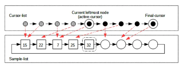
that left(1/λ) is the entire sample-list. For eachi(1 ≤i≤1/λ), we associate a random walk on left(i) (we call iti-walk) based on algorithm Step. Thus we have1/λwalks. We allocate another list of1/λmemory positions calledcursor-list. As with the sample-list, a number (between 1 and1/λ) is implied for each node of the cursor-list, according to the order (from left to right) of the nodes in the list.∀i(1≤i≤1/λ), thei-th node of the cursor-list is going to host the cursor of thei-walk.
Ifielements of the stream have been inserted into the sample-list, they occupylef t(i)
and thei-walk is theactive-walk. Initially, since no stream element exists in the sample, all walks areinactiveand clearly, if thei-walk is active, then all thej-walks(1≤j < i)
have been active in the past. When thei-walk becomes inactive, the (i+ 1)-walk will become active. Keep in mind that although we have defined1/λwalks, we need to keep track of only two walks: the active-walk and the(1/λ)-walk.
When a walk becomes inactive, we free the node of the cursor-list corresponding to the cursor of this walk. As a result, the nodes of the cursor-list are set free in left to right order and at all times, the leftmost node of the cursor-list contains the cursor of the active walk (we call this pointeractive-cursor). This means that we are able to access the active-cursor in constant time. It is also clear that the rightmost node of the active-cursor-list contains the cursor of the(1/λ)-walk (we call this cursor final-cursor). Thus, by maintaining a pointer towards this node, we are able to access the final-cursor in constant time. Finally, we maintain a pointer calledactive-limit, towards the rightmost node of the active walk (i.e. if thei-walk is the active walk, we maintain a pointer towards thei-th node of the sample-list).
Before the elements of the stream start to arrive we have thepreprocessing phase
where we traverse the cursor-list from left to right and store in thei-th node, a pointer to a position of the sample-list, chosen uniformly at random among all sample-list positions between 1 andi. After this task is completed,∀ i(1 ≤ i ≤ 1/λ), thei-th node of the cursor-list contains the cursor of thei-walk. For the preprocessing phase we useO(1/λ·
log (1/λ))random bits. Assuming that each random bit costsO(1)time, the worst-case time complexity for the preprocessing phase isO((1/λ)2·log (1/λ))because for each
iwe need to traverse the sample-list from node 1 to nodeiin order to access the node chosen uniformly at random among all the nodes from node 1 to nodei.
The above description is depicted graphically in Figure 2. According to the figure, the active walk is the 5-walk, the filled nodes of the sample-list are represented through rectangles and the empty ones through circles. Above the sample-list, we illustrate the cursor-list. The shaded nodes on the left part of the cursor-list have been deleted in the past, and the leftmost (black) node contains the cursor of the active-walk. The highlighted node of the sample-list is pointed by the active-limit pointer. The sample-user of limited access can only see the sample-list and since the active-limit pointer is “out of sight”, no node of the sample-list appears highlighted to the sample-user of limited access.
Fig. 2.The background for introducing Algorithm 2.
Algorithm 2. WhenS(t+ 1) arrives, we deterministically add it to the sample.Ifthe final-cursor points to a non-empty position of the sample-list, the new stream element is going to replace an existing element of the sample i.e. the number of elements in the sample will remain the same. We execute a step for thei-walk and appropriately update the active-cursor. Letgbe the node pointed by the active-cursor. The previous node ofg
is the hit-node of the step, and letxbe that node. We deletexfrom the sample-list by connecting the previous node ofxtog. Then, we insert xbetweenw andz. We store
S(t+ 1)inx. We set theactive-limitpointer to point tox.Elsethe number of elements in the sample will increment and the(i+ 1)-walk will become the active-walk. We insert
S(t+ 1)inz. We delete and free the leftmost node of the cursor-list, making the (i+ 1)-th walk to be the active walk. We update the active-limit pointer to point toz.End-If. We execute a step for the(1/λ)-walk.
A first observation is that the elements are stored in increasing arrival order, from left to right. Clearly, the space-complexity isO(1/λ)dominated by the length of the two lists. In practical terms, the entire used-space is initially twice the space of the sample-list. However, each time the number of elements inside the sample increases, we free the leftmost node of the cursor-list and as a result, the entire used-space decreases over time. When the entire sample-list is filled with elements, only one node from the cursor-list remains. It is the node that contains the cursor of the(1/λ)-walk. This means that in regard to Algorithm A, the only memory overhead that remains is the one due to the pointers that support the sample-list. Concerning the time complexity, Algorithm 2 clearly usesO(1)random bits per stream element and beyond that, all the other actions costO(1)
time. Assuming that each random bit costsO(1)time, our algorithm needs constant time per stream element in the worst-case.
Theorem 3 Associating Algorithm 2 with the exponential bias function, Algorithm 2 con-vinces a sample-user of limited access.
active-walk, the active-cursor was set to point to a node of thei-walk chosen uniformly at random. Not being able to access the active-cursor, the user concludes that it may point to any node of thei-walk with probability1/i, because the Markov chain associated with this walk has reached its stationary distribution and obviously, each step from that point and on cannot change the distribution. Let us now assume that the current time ist, the length of the sample-list isnand the fraction of the sample-list occupied by elements is
F(t)(note that at this point, the proof of Theorem 2.2. in [1] starts). Then, according to the algorithm, whenS(t+ 1)arrives, an element of the sample is going to be deleted with probabilityF(t)and if such a deletion is decided, each of then·F(t)elements of the sample have equal probability1/(n·F(t))of being deleted (because, as stated above, the cursor may point to each position with equal chances). As a result, the probability of an element being deleted isF(t)(1/(n·F(t))) = 1/n. It follows that the probability of a stream element to survive att+ 1is1−1/n. Thus, the element that arrives at timerwill survive in the sample at timet with probability(1−1/n)t−r = ((1−1/n)n)(t−r)/n. For large values ofn, the inner(1−1/n)nterm is approximately equal to1/e, and from substitution, the exponential bias function follows (note that at this point, the proof of Theorem 2.2. in [1] ends). In advance, the user cannot decide on the position of the walk for any future time-point and as a result, whatever holds for the existing sample-elements
also holds for the future sample-elements.
One issue of interest to be discussed is the following: The walk of Section 5 is defined on a static list. According to Algorithm 2, we are able to delete an internal node of the list and re-insert it as the new rightmost node of the active walk. This results in the position of the active-walk moving one node to the left. The same holds for the position of the
(1/λ)-walk. This is not the walk we presented in Section 4. In particular it now follows that in each step the probability of doing nothing i.e. going one position forward and then one position backwards (thus ending up at the starting point) is 1/2, the probability to move one node to the right is 1/4 and so on. This is a lazy version of our walk and it is trivial to see that in this lazy version the stationary distribution remains the same. Thus, Algorithm 2 is not affected.
Going to the greedy approach is trivial. It turns out that we do not need the cursor-list, but instead only the cursor for the(1/λ)-walk. Therefore, the space remains the same and equal to the final space consumed by the strict approach. The time complexity remains identical to that of the strict approach.
7.
Discussion
our algorithms to create samples consistent with the exponential bias function. In other words, survival probabilities are decided when the algorithm is created. It then follows that the randomness used in [1] is more than the randomness we really need in order to obtain a biased sample. It is a sample-user of limited access that we actually have to convince, and not a sample-user of full access. This observation has led to optimal randomness complexity for the problem we are studying and we believe that the technique we use for introducing randomness to our algorithms (i.e. the notion of limited access) may be useful in other problems.
References
1. Aggarwal C. C.: On biased reservoir sampling in the presence of stream evolution. In proceed-ings of the 32nd international conference on Very large data bases , pp. 607–618. Seoul, Korea (2006).
2. Aggarwal C. C. and Yu P. S.: A Survey of Synopsis Construction in Data Streams. Data Streams - Models and Algorithms, pp. 169–207 (2007)
3. Babcock B., Datar M. and Motwani R.: Sampling from a Moving Window over Streaming Data. In proceedings of ACM-SIAM Symposium of Discrete Algorithms, pp. 633–634, San Francisco, USA (2002).
4. Babu S. and Widom J.: Continuous queries over data streams. ACM SIGMOD Record Archives, Volume 30, Issue 3, pp 109–120 (2001).
5. Chung F. R. K. , Graham R. L. and Yau S.-T.: On Sampling with Markov Chains. In proceed-ings of the seventh international conference on Random structures and algorithms, pp. 55–77, Atlanta, USA (1996).
6. Gibbons P. and Mattias Y.: New Sampling-Based Summary Statistics for Improving Approxi-mate Query Answers. In proceedings of ACM SIGMOD, pp. 331–342, Seattle, USA (1998). 7. Gibbons P.: Distinct sampling for highly accurate answers to distinct value queries and event
reports. In Proceedings of 27th International Conference on Very Large Data Bases, pp. 541– 550, Rome, Italy (2001).
8. Goldreich O.: Another Motivation for Reducing the Randomness Complexity of Algorithms. Studies in Complexity and Cryptography. Miscellanea on the Interplay between Randomness and Computation, pp. 555–560, (2011).
9. Jerrum M. and Sinclair A.: Conductance and the rapid mixing property for Markov chains: the approximation of permanent resolved. In proceedings of the twentieth annual ACM Sympo-sium on Theory of Computing, pp. 235–244. Chicago, USA (1988).
10. Hellerstein J., Haas P. and Wang H.: Online Aggregation. In proceedings of ACM SIGMOD, pp. 171–182, Tucson, USA (1997).
11. Lawler G. F. and Sokal A. D.: Bounds on theL2Spectrum for Markov Chains and Markov Pro-cesses: A Generalization of Cheeger’s Inequality. Transactions of the American Mathematical Society Vol. 309, No. 2, pp. 557–580 (1988).
12. Manku G. and Motwani R.: Approximate Frequency Counts over Data Streams. In proceedings of the 28th International Conference on Very Large Data Bases, pp. 346–357, Hong Kong, China (2002).
13. Manku G., Rajagopalan S. and Lindsay B.: Random Sampling for Space Efficient Computation of order statistics in large datasets. In proceedings of ACM SIGMOD, pp. 251–262, Philadel-phia, USA (1999).
15. Montenegro R.: Intersection Conductance and Canonical Alternating Paths: Methods for Gen-eral Finite Markov Chains. Combinatorics, Probability and Computing, Volume 23, Issue 4, pp. 585–606 (2014).
16. Vitter J. S.: Random sampling with a Reservoir. ACM Transactions on Mathematical Software, Volume 11 Issue 1, pp. 37–57 (1985).
17. Wu Y., Agrawal D. and Abbadi A.: Applying the Golden Rule of Sampling for Query Estima-tion. In proceedings of ACM SIGMOD, pp. 449–460, Santa Barbara, USA (2001).
A.
The intuition on Algorithm Step
In order to give the intuition behind this algorithm, let us name the list L. Let us set
length(L) = 5andK =length(L)i.e., the maximum number of coin-tosses per step is 5. We assume that time increments (starting from 0) with each step, and suppose that someone is trying to guess the node pointed by the cursor, without accessing the cursor. At time 0, the node pointed by the cursor can be deterministically determined because the cursor points to the head of the list. Now, let us “travel” into the future and make our first stop at time-point 1. The probabilities for the cursor to point to each node at time 1 are shown in the following table (where “T” stands for “tails” and “H” stands for “heads”) and let us be a bit more detailed on how these probabilities are derived: Let us focus on the probability that the cursor points to Node 1 at time-point 1. It follows that the execution of Step() that moved the cursor (starting from Node 1) back to Node 1 contains as many coin-tosses as necessary for the cursor to complete the circle. This means that the first coin-toss cannot cannot result to “heads” because then, the cursor will stop at Node 2 (keep in mind that a step ends when the coin-toss results to “heads” or when 5 coin-tosses have occurred). Given that the first coin-toss results to “tails” the second coin-toss cannot result to “heads” because then the cursor will stop at Node 3 (therefore the event “TH” leads to Node 3). Following this logic we conclude that in order for the cursor to complete a full circle, either the event “TTTTT” or the event “TTTTH” must occur during the first execution of Step(). The probability of each of these two events to occur is 1/32. We conclude that the probability for the cursor to return to Node 1 at time-point 1 is1/16.
Node 1 Node 2 Node 3 Node 4 Node 5
P1,1 = 1/16 (event TTTTT OR TTTTH)
P2,1 = 1/2 (event H)
P3,1 = 1/4 (event TH)
P4,1 = 1/8 (event TTH)
P5,1 = 1/16 (event TTTH)
As time passes i.e. as more steps are performed, coin tosses gradually insert random-ness into the scheme, introducing an increasing uncertainty on the position of the cursor. The probabilities at time-point 2 are shown below.
P1,2=P1,1∗1/16 +P2,1∗1/16 +P3,1∗1/8 +P4,1∗1/4 +P5,1∗1/2
P2,2=P2,1∗1/16 +P3,1∗1/16 +P4,1∗1/8 +P5,1∗1/4 +P1,1∗1/2
P3,2=P3,1∗1/16 +P4,1∗1/16 +P5,1∗1/8 +P1,1∗1/4 +P2,1∗1/2
P4,2=P4,1∗1/16 +P5,1∗1/16 +P1,1∗1/8 +P2,1∗1/4 +P3,1∗1/2
P5,2=P5,1∗1/16 +P1,1∗1/16 +P2,1∗1/8 +P3,1∗1/4 +P4,1∗1/2 In general, for time-pointi, we have:
P1,i=P1,i−1∗1/16 +P2,i−1∗1/16 +P3,i−1∗1/8 +P4,i−1∗1/4 +P5,i−1∗1/2
P3,i=P3,i−1∗1/16 +P4,i−1∗1/16 +P5,i−1∗1/8 +P1,i−1∗1/4 +P2,i−1∗1/2
P4,i=P4,i−1∗1/16 +P5,i−1∗1/16 +P1,i−1∗1/8 +P2,i−1∗1/4 +P3,i−1∗1/2
P5,i=P5,i−1∗1/16 +P1,i−1∗1/16 +P2,i−1∗1/8 +P3,i−1∗1/4 +P4,i−1∗1/2 It is not difficult to write a simple program and see that these probabilities converge to 1/5, as time progresses. Thus, after “a while”, enough randomness has been inserted, for the cursor to be in each position with equal chances.
B.
Bounding the mixing time
Bounding the mixing time of a Markov chain can be difficult. Here, we will use the con-ductance method ([9], [11]), according to which the ergodic flow between two subsets
S, T ⊂V is defined to be
Q(S, T) = X
i∈S,j∈T
πiPij
The method could bound the mixing time for lazy reversible Markov chains, but it was extended in [15] in order to apply to general finite ergodic Markov chains. According to [15], theintersection conductanceΦˆ(A)ofA⊂ V (andA¯, the complement ofA) is given by
ˆ
Φ(A) = ˆΦ(A,A¯) = P
u∈Vmin{Q(A,u),Q( ¯A,u})
2π(A)π( ¯A)
Then, the intersection conductance isΦˆ = min ∅(A(V
ˆ
Φ(A). In [15] it is proved that the mixing time of a finite ergodic Markov chain is
r()≤ 12 ˆ Φ2log
1 √π0
whereπ0= minu∈Vπu.
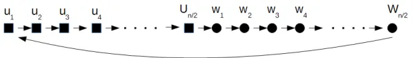
We are first going to bound the mixing time for K = 2, i.e. if at most 2 coin tosses are allowed in algorithm Step. For every i, j ∈ V, ifpij = 1/2, we say that state j is thenextof i. The left part of Figure B.1 visualizes the walk on 7 nodes. The black arrows correspond to probabilities of 1/2 and the red ones to probabilities of 1/4. The “contribution” of a nodeuin the numerator ofΦˆ(A), depends on the status of the three “preceding” nodes (according to the order defined by the black arrows). We distinguish 8 cases, depending on whether each of the 3 nodes belongs to A, or toA¯. We name each case through the corresponding 3-bit number (each node corresponds to a 1, if it belongs toA, or to a0, otherwise).
Let us introduce the following terminology: Set A outperforms setB, ifΦˆ(A) ≤
ˆ
Φ(B). LetA⊂V. Then, if all the states ofAare connected through probabilities of 1/2, we call the set,tight. We are now ready to bound the mixing time of the Markov chain assuming thatK= 2.
Theorem B 1 SettingK = 2,r() =O(n2logn), wherenis the number of states and
Fig. B.1.The random walk for 2 coin tosses. On the right, we show all the possible addi-tives in the nominator ofΦˆ(A), because of nodeu.
Proof. We need to find the setAthat outperforms all other sets. Let us first consider all the sets that containdstates, for a givendsuch that1< d≤n/2(by allowingAto contain more nodes,A¯contains less thann/2nodes and by renamingAtoA¯andA¯toA, we fall into the same case). Thus, letAbe such a set of cardinalityd. Then, the denominator in
ˆ
Φ(A)is2·d n·
n−d
n . Since all the sets of cardinalitydproduce the same denominator, the one that results to the smallest numerator outperforms all the others. Observe, that in Figure B.1, the contribution of a node to the numerator ofΦˆ(A)is 0 if the three preceding states either all belong toA, or all belong toA¯. As a result, among all the sets of cardinalityd, the ones that outperform all the others are the tight ones. This is because in this case, the number of states for which the three preceding states either belong toAor not, maximizes and thus the numerator is minimized. For example, in Figure B.2 the states represented by squares belong toA, and the states represented by circles belong toA¯. It follows that only
u2, u3, w2andw3will contribute to the numerator. In particular, foru2we have the case 001 (see Figure B.1), foru3we have the case 011, forw2 we have case 110 and forw3 we have case 100. Observe that ifA, Bare tight sets (of states) of the same cardinality, thenΦˆ(A) = ˆΦ(B).
We have now concluded that among all the sets of states having the same cardinality, anyone that is tight outperforms all the others. As a result, instead of trying to find the set
Athat minimizesΦˆ(A)among all possible sets, we need to examine only the tight ones. Observe now that all the tight sets of more than two states produce the same numerator. As a result, among all the tight sets with more than two states, we must find the ones that result to the maximum denominator in order to minimize the fraction. The denominator is maximized for any set havingn/2states. We have now concluded that ifAis tight and containsn/2 states andB is any other set of states that contains more than two states,
ˆ
Fig. B.2.The rectangles correspond to the states ofA. The arrows corresponding to prob-abilities with value less than 1/2 are omitted.
ˆ
Φ(A) = 41n+
1 2n+
1 2n+
1 4n
21 2 1 2
= 3n.
It remains to see if there is a tight set of cardinality 1 or 2 that outperforms the tight sets of cardinalityn/2. For any tight setBof cardinality 2, only four nodes will contribute to the numerator ofΦˆ(B). In particular, the second (according to the order of the black arrows) node ofB will fall into case 001, and the next three nodes (that belong toB¯) will fall into cases 011, 110 and 100, respectively. It follows that for any tight setB of cardinality 2:
ˆ
Φ(B) = 8(n3n−2).
Similarly, for any single state setC, only the three states after the one that belongs to
Care going to contribute to the numerator and they are going to fall into cases 001, 010 and 100 (according to the order defined by the black arrows). Thus, for any single state setCwe have:
ˆ
Φ(C) =
1 2n+
1 4n+
1 4n
21
n n−1
n
=2(nn−1).
It follows that any tight setAof cardinalityn/2outperforms all tight sets of cardinal-ity 1 and 2 for alln≥8, and as a result, it outperforms any other set of states. We have now concluded that by allowing at most two coin tosses,Φˆ= n3. This means that setting
= 1/ncfor some constantc, we getr()∈O(n2logn).
It remains to find the mixing time forK >2. Clearly, by increasingKwe increase the area that each step can cover, and thus it is a fact that the mixing time is going to improve. However, asymptotically things remain the same, as the next theorem states. Theorem B 2 SettingK =n,r()∈O(n2logn), wherenis the number of states and
n≥8.
c, 12 ( ˆΦ(A))2 log
1
√π0 = O(n
2logn). For the description we are going to use Figure B.2, where the states ofAappear as rectangles, and the states ofA¯appear as circles. Keep in mind that the arrows corresponding to probabilities with value less than 1/2 are omitted, however sinceK = n, each state is actually connected to all the other states. For states fromw2untilu1(following the arrows of probability 1/2), it is the setAthat contributes to the numerator ofΦˆ(A). For states fromu2untilw1it is the setA¯that contributes to the numerator ofΦˆ(A). In particular:
Nodew2contributesn1(14+18+· · ·+ 1 2n2+1)<
1 2n Nodew3contributesn1(18+161 +· · ·+ 1
2n2+2)< 1 4n · · · ·
Nodeu1contributesn1(n1
2+1
+ 1
n
2+1
+· · ·+ 1 2n)<
1 n2n2
It follows that the total contribution of all the states fromw2tou1is smaller than 1n. Examining the remaining states (i.e. fromu2tow1), the results are identical. It follows that when setAis a tight set ofn/2edges we have the following:
ˆ
Φ(A)< n2
21 212
= 4
n. Observe that the following also holds:Φˆ(A) =O( 4 n) As a result, by setting = 1/nc for some constantc, we get 12
( ˆΦ(A))2log 1 √π0 =
O(n2logn).
George Lagogianniswas born in Xylokastro, a small town located in the north-east coast of Peloponnisos, Greece. He is an assistant professor at the department of Agricultural Economics and Rural Development in the Agricultural University of Athens. His research is focused on the field of data structures and algorithms.
Stavros Kontopoulosis a Phd student in the area of distributed indexing structures. His interests among others are: distributed system design, data streaming technologies, and NoSql databases. He is also a software engineer with more than 10 years of experience in various industries. His current focus is on machine learning and data streaming.
Christos Makrisis an Associate Professor in the University of Patras, Department of Computer Engineering and Informatics, from September 2017. Since 2004 he served as an Assistant Professor in CEID, UoP, tenured inthat position from 2008. His research interests include Data Structures,Information Retrieval, Data Mining, String Processing Algorithms, Computational Geometry, Internet Technologies, Bioinformatics, and Mul-timedia Databases. He has published over 100 papers in refereed scientific journals and conferences and has more than 600 citations excluding self-citations (h-index:16).