Formulation Optimization of Polyox Based Modified Release Drug Delivery System

(1)

ISSN: 2250-1177 [551] CODEN (USA): JDDTAO Available online on 19.08.2019 at http://jddtonline.info

Journal of Drug Delivery and Therapeutics

Open Access to Pharmaceutical and Medical Research

Open Access

Research Article

Formulation Optimization of Polyox Based Modified Release Drug Delivery

System

**Shah Sunil, Shukla Dilip*, Pandey Harish**

Sri Satya Sai University of Technology & Medical Sciences, Sehore (M.P), India-466001

ABSTRACT

Polyethylene Oxide (PEOs) offer specific advantages to be used in pharmaceutical products as release modifiers by forming a hydrogel around the dosage form in aqueous environment causing the drug to follow a diffusional path before releasing into the media. The strength of the hydrogel governs the release retardation capacity of the PEO system. The objective of this dissertation work was to use the Design of Experiments methodology to develop and optimize a PEO based modified release formulation of a highly water-soluble drug like Metoprolol succinate. The effect of the different viscosity grade PEOs, their concentration with respect to the drug, combination of two different viscosity grades, % drug content in the formulation and the use of water soluble / insoluble fillers on the dissolution of metoprolol succinate was studied. The critical formulation parameters namely PEO concentration and % drug content were chosen as input factors and dissolution at 1, 4, 8 and 20 hours was recorded as responses to carry out optimization using the DOE approach. The results obtained after statistical treatment of data provided a design space that can be used for achieving the desired formulation profile. The model has been validated to predict the effect of the input factors (PEO type and concentration and % drug content) on the responses (in vitro dissolution).

Keywords: Polyethylene Oxide, Modified Release Drug Delivery System, Metoprolol

Article Info:Received 19 June 2019; Review Completed 26 July 2019; Accepted 06 Aug 2019; Available online 19 August 2019

Cite this article as:

Shah S, Shukla D, Pandey H, Formulation Optimization of Polyox Based Modified Release Drug Delivery System, Journal of

Drug Delivery and Therapeutics. 2019; 9(4-s):551-561 http://dx.doi.org/10.22270/jddt.v9i4-s.3383

*Address for Correspondence:

Dilip Shukla, Research Scholar, School of Pharmacy, SSSUTMS, Sehore- MP (India)- 466001

INTRODUCTION

Modified drug delivery is a domain which requires high degree of skill and understanding in order to regulate the release of the pharmaceutical compound. More often than not, the therapeutic dosing requirement governs whether a particular compound has to be given as a modified drug delivery or as a conventional immediate release dosage form. There can be numerous reasons due to which, the rate of release of the drug from the dosage form needs to be controlled; Primary being to have the drug into systemic circulation at a constant rate for a prolonged period of time so that it elicits a continuous pharmaceutical activity. The drugs with shorter half life, higher doses with narrow therapeutic window, are ideal candidates for delivery as modified release systems. In order to formulate a modified release delivery system, the right combination of scientific principles can in turn help effect the desired kind of release of the drug from the dosage form and thus deliver the drug at the rate and amount as desired or as most beneficial to

the body1-3_{. Based on the mechanism of drug release from}

the modified release drug delivery systems, they can be classified as Diffusion controlled (matrix and reservoir type

of systems) Dissolution controlled, (surface eroding, surface swelling type of systems), Osmotic drug delivery, Multi particulate systems, Enteric coated (pH dependent systems). Generally, the mechanism of drug release from any kind of modified release delivery system is governed by either of the above mechanisms. The regulation of drug release is achieved by incorporating release retarding agents into the formulations. The most widely used release retarding agents are polymers like high viscosity HPMC for diffusion and dissolution-controlled systems, or pH sensitive polymers like Eudragits and Ethyl cellulose for enteric coated and Multi particulate systems. Osmotic drug delivery systems involve controlling the release by incorporating an osmogen and a semi permeable membrane into the formulation in order to have a zero order

continuous release from the medication 4-6_.

(2)

ISSN: 2250-1177 [552] CODEN (USA): JDDTAO and help in retarding the release of the API from the

formulation. They are available in various different viscosity grades based on their molecular weights. They are relatively easy to process into dosage forms because of their free flowing and directly compressible nature and can be used as mere fillers in the tablets in order to act as release retardants. Thus, using PEOs in the formulation does not involve complex set of criticial process variables as observed in case of preparing a matrix, reservoir or a MUPS

based delivery system7-9_{. The purpose of this Research}

work would be to apply design of experiments (DOE) approach to development and optimization of a Polyox based modified release drug delivery system of a highly water-soluble drug. In order to evaluate the effect of Polyox on the release modulation of the drug in the formulation, a model drug was chosen by screening a variety of drug molecules to meet certain pre-defined criteria as mentioned below

 High solubility and high permeability i.e. BCS class I

drug. (i.e absorption is not solubility or permeability dependent).

 Biological half life (t1/2) between 2-6 hours to avoid

accumulation in the body. Shorter t1/2 will ensure rapid

clearance after absorption, thus negating any dose related side effects.

 Moderate dose of between 50-150 mg per unit.

 Drug for which use of extensive and elaborative coating

process may not be a feasible approach.

Based on the above criteria, Metoprolol succinate was selected as a model drug to evaluate and optimize the formulation related variables associated with polyethylene oxide.

MATERIALS AND METHODS

Materials: The Active pharmaceutical ingredient -

Metoprolol succinate used for the study was manufactured by Ipca Laboratories Ltd. Polyethelene oxide polymers were obtained as gift samples from Alpa laboratories ltd India. The other ingredients Prosolv HD 90, directly compressible lactose (Supertab 21), and magnesium stearate were purchased from sources JRS Pharma, Fontenna Excipients and Signet Pharma respectively by Ipca laboratories ltd.

Process of preparation of experimental formulations:

The process of preparation of the formulations involved dispensing of raw materials and active, followed by co-sifting, mixing and then compression into tablets. A brief step wise description of the manufacturing process is as mentioned below.

Procedure: Dispense the drug substance as per batch requirement. Sift the drug substance through a # 50 sieve. Dispense the excipients (PEO, Prosolv HD 90 or DCL 21) as per batch requirement.

Co-Sift the excipients along with API through # 50 sieve 2 -3 times. Load the blend into the blender and Mix blend for 10 min. Add required quantity of magnesium stearate (sifted through # 50 sieve) and blend for another 5 min. Compress tablets equivalent to make 100 mg Metoprolol succinate. A flow chart of the manufacturing procedure is depicted below.

Figure 1: Flow chart for manufacturing of Metoprolol succinate PEO tablets

Analytical methodology: The analytical methodology

for in vitro drug dissolution was adapted from the Official USP monograph for Metorpolol succinate extended release tablets. The tablets were analyzed for content of metoprolol succinate in the dissolution medium. The details of the method are as mentioned below

In vitro Dissolution method: The in vitro dissolution analysis was carried out in pH 6.8 phosphate buffer, 500 ml in USP type II paddle Apparatus at 50 rpm. The samples were withdrawn using auto sampler at 1, 4, 8, 12, 20 hours. The volume of samples withdrawn was replaced by additional media from replacement bowl.

HPLC analysis: The HPLC analysis was carried out using a 4 mm X 12.5 cm column containing C18 packing. The mobile phase of pH 3.0 phosphate buffer: Acetonitrile (375:125) was used for elution at a flow rate of 1 ml/min. The wavelength of absorption was determined using a PDA detector in the HPLC where Metoprolol succinate showed two maxima at wavelengths of 222 nm and 275 nm. The 222 nm maxima showed a greater response and hence it was chosen as the wavelength for estimation for all the dissolution samples.

Preparation of pH 3 Phosphate buffer: Mixed 50ml of 1M monobasic sodium phosphate and 8.0 ml of 1M phosphoric acid and diluted with water to 1000 ml. Adjusted pH to 3.0 with 1M monobasic potassium phosphate or 1M phosphoric acid.

Preparation of standard solution: Dissolved 50 mg accurately weighed Metoprolol succinate in Mobile Phase to obtain a solution of known concentration of about 0.05 mg per ml (i.e. 50 ppm). 20 µl of injection volume was used to determine the response.

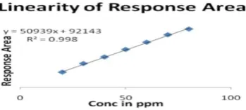
Preparation of sample solution: The 2 ml aliquot from the samples collected in at each time point in dissolution vial and diluted with the dissolution medium to 5 ml in a volumetric flask. Injected 20 µl of sample solution in the HPLC column. The standard curve was prepared to determine the linearity of the response area (area under the peak) across different concentrations and the R2 value was found to be 0.998. The figure 2 below depicts the standard linearity graph.

(3)

ISSN: 2250-1177 [553] CODEN (USA): JDDTAO

Figure 3: Chromatograms of the standard, blank and sample

RESULTS AND DISCUSSION

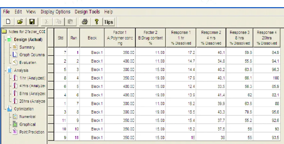
The results of the experimental formulations were compiled in the DOE response sheet in the Design expert ® software screen as mentioned in the Figure 4 below and the

further subjected to data treatment to arrive at statistically significant factors that impact the formulation design. The

12th_{hour dissolution was performed only to arrive at}

profile across the time range but this response was not used for data analysis and optimization in the DOE.

Figure 4: DOE Experimental design and responses

The Quadratic model was chosen for fitting the data as it is the most preferred model for fitting the CCD design and no aliases were found in the model. Since the model chosen is quadratic, a second order polynomial would be used for predicting the response functions.

Y = β0 + β1A+β2B+β3A2_+β4B2_+β5AB

Where, Y is the response, A and B are independent variables and β0 to β5 are the constants or coefficients

(4)

Table 1: Response compilation in DOE

Name Units Type Desired

Response Low High Std. Dev Ratio of Max To min

Polymer conc mg Factor - 300 400 NA NA

Drug content % Factor - 11 19 NA NA

1 hrs % Dissolved Response < 25 % 12.4 19 0.3006 1.492

4 hrs % Dissolved Response 20 – 40 % 33.5 43.3 2.0381 1.293

8 hrs % Dissolved Response 40 – 60 % 55 70.6 1.6746 1.284

20 hrs % Dissolved Response 80 – 100 % 82.1 100 4.3736 1.218

The results obtained for each of the responses are mentioned in the table 2. The selected model for each response is underlined.

Table 2: Sequential Model sum of Squares

Response Model F Value P value

D @ 1 hour

Linear 2.26 0.1665

2FI 0.92 0.3704

Quadratic 99.06 <0.001

Cubic 0.18 6.61

D @ 4 hours

Linear 5.77 0.02

2FI 0.58 0.4696

Quadratic 3.82 0.0983

Cubic 46.37 * 0.0055

D @ 8 hours

Linear 5.54 0.0309

2FI 5.46 0.9432

Cubic 0.0043 0.9589

D @ 20 hours

Linear 1.25 0.3368

2FI 5.02 0.0600

Cubic 282.36 * 0.0004

* cubic model is aliased for a central composite design. Hence design augmentation required to remove the alianses and estimate the higher order terms. Hence here, the next best F value model is selected for evaluation.

The complete ANOVA output for all the responses is described later in table 3, 4 and 5. Here also a higher F value and p value less than 0.1 (preferably < 0.05) indicates a significant model chosen for the data.

Table 3: ANOVA output for response surface - Model

Response Model Model F

Value P value model terms Significant Final equation in terms of coded factors

D-1 hour Quadratic 70.92 0.001 A, B, AB, A2,

B2 +15.18-1.35* A+0.37* B-0.78* A * B 1.76*A2_{+2.39* B2}

D-4 hours Linear 5.77 0.02…81 A, B +38.77 -2.28*

A+1 .67 * B

D-8 hours Quadratic

with model reduction for A2

14.51 0.0031 A, B, B2 +57.22-3.98*A

+3.28* B - 0.15 * A * B + 5.73 * B2

D-20 hours 2 FI 2.93 0.109 A, B +91.45 -2.97 * A +

1 .78* B-4.90*A * B If extra design points beyond what‘s needed for the model

are added, and some points were replicated to provide an estimate of pure error, the results of a Lack of Fit test for each model also can be calculated. Lack of Fit compares the residual error (MEAN SQUARE) to the pure error (MEAN

SQUARE). Lack of fit is NOT desirable so a small F value and p value greater than 0.05 (preferably < 0.1) are desired. If a model shows significant lack of fit, it should not be used to predict the response. The lack of fit calculation for the four responses is described in the table 4 below.

Table 4: Model Lack of Fit calculation for four responses

Response Model Chosen F Value P value Character

D @ 1 hour Quadratic 3.10 0.2534 In-significant

D @ 4 hours Linear 87.12 0.1114 Marginally Significant

D @ 8 hours Quadratic 16.03 0.0593 In- significant

D @ 20 hours 2FI 131.30 0.0076 Significant

The other objective can be where the primary concern is to simply identify factors and interactions that are affecting the response and generally just learn if higher or lower factor levels are better (generally with factorial designs). In this case, there might have the situation where the model is statistically significant and there is no lack of fit, but the R-squared's are low. It can be concluded that the significant terms identified are correct and the graphs will show the

(5)

ISSN: 2250-1177 [555] CODEN (USA): JDDTAO on in totality. A good next step would be to set the known

factors at their best settings and then brain-storm about other possible factors and run another DOE. The R square

values for all four responses are compiled in the table 5 below.

Table 5 : R2 Values for all four responses

Response R2 R2 Adjusted R2 Predicted Adequate precision PRESS

D @ 1 hour 0.9861 0.9722 0.8745 28.065 4.08

D @ 4 hours 0.5906 0.4883 0.1117 7.442 71.63

D @ 8 hours 0.9861 0.9043 0.8439 12.225 56.26

D @ 20 hours 0.5564 0.3332 -0.9814 5.996 598.05

As is described in the table above, the cubic model showed better F values fo the D@4 hours and D@20 hours indicating higher order terms impacting the responses. Since the D@ 20 hours response is the final time point in the dissolution and the specification of Dissolution > 80% meets for all points across the design points this response need not be used for predictive purposes. Also, the low predictability observed for D@4 hours can be overlooked as it has a brackting of D@1 hour and D@8 hours which in turn can be predicted acturately from the model. But a final full proof solution to better fitting of data to all responses

would be to augment the design to better estimate higher order terms to fit the cubic model to these two responses. The current work limits to identification of the significant factors for responses D@4 hours and D@20 hours and ascertains that the predictive power of the model is low for these responses.

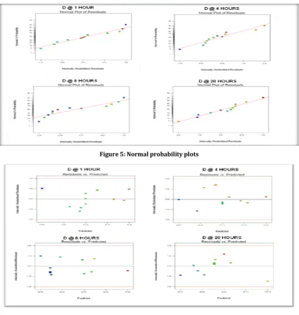
The normal probability The Normal probability plots for the four responses are plotted in figure 5 & 6 depict that the distribution is uniform and there is no specific pattern in the distribution.

Figure 5: Normal probability plots

(6)

ISSN: 2250-1177 [556] CODEN (USA): JDDTAO The DOE software analyses the differences between the

actual values obtained for experimental runs and the predicted values one would have arrived at if the models

were used to predict the response at the set of factor combinations corresponding to the runs. The details for each of the responses are compiled in the table 6 and 7.

Table 6: Predicted vs Actual Compilation – Response D@ 1hour and D@ 4 hours

Standard Order

D @ 1 Hour D @ 4 Hours

Actual

value Predicted value Residual Actual value Predicted Value Residual

1 16.2 16.0214 0.178 39.9 39.389 0.510

2 14.7 14.8714 -0.171 34.8 34.822 -0.022

3 18.5 18.3048 0.195 43.3 42.722 0.577

4 13.9 14.0548 -0.154 41.4 38.156 3.243

5 14.4 14.7736 -0.373 40.2 41.056 -0.856

6 12.4 12.0736 0.326 33.5 36.489 -2.989

7 17.2 17.2070 -0.007 40.1 37.106 2.993

8 17.9 17.9403 -0.0403 40.1 40.439 -0.339

9 15 15.1842 -0.184 38 38.772 -0.772

10 15.2 15.1842 0.0157 37.5 38.772 -1.272

11 15.4 15.1842 0.215 37.7 38.772 -1.072

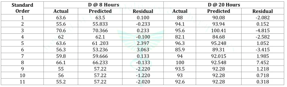
Table 7: Predicted vs Actual Compilation – Response D@ 8 hour and D@ 20 hours Standard

Order Actual D @ 8 Hours D @ 20 Hours

value Predicted value Residual Actual value Predicted value Residual

1 63.6 63.5 0.100 88 90.08 -2.082

2 55.6 55.833 -0.233 94.1 93.94 0.152

3 70.6 70.366 0.233 95.6 100.41 -4.815

4 62 62.1 -0.100 82.1 84.68 -2.582

5 63.6 61 .203 2.397 96.3 95.248 1.052

6 56.3 53.236 3.063 85.9 89.31 -3.415

7 59.8 59.666 0.133 94 92.015 1.985

8 66.1 66.233 -0.133 100 92.548 7.452

9 55 57.22 -2.220 93.5 92.28 1.218

10 56 57.22 -1.220 93 92.28 0.718

11 55.2 57.22 -2.020 92.6 92.28 0.318

The residual values in the tables above indicate that there is no significant variation in the actual responses obtained and those predicted by the model. The Predicted Vs Actual plots for all responses are depicted in the figure 7. It can be observed that the predicted vs actual point are more closer to the line for responses D@ 1 hour and D @ 8 hours indicating better fit of model to the data. The points are more

(7)

Figure 7: Predicted vs Actual Plots

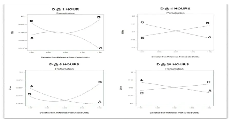
The perturbation plot helps to compare the effect of all the factors at a particular point in the design space. The response is plotted by changing only one factor over its range while holding of the other factors constant. By default, Design-Expert software sets the reference point at the midpoint (coded 0) of all the factors. But it can be changed to any point (perhaps the optimal run conditions) by using other Factors Tool in the software. A steep slope or curvature in a factor shows that the response is sensitive to that factor. A relatively flat line shows insensitivity to change in that particular factor. If there are more than two

factors, the perturbation plot could be used to find those factors that most affect the response. These influential factors are good choices for the axes on the contour plots. This plot is like "one factor at a time" experimentation – it does not show you the effects of interactions. Since this study was carried out with only two factors, the perturbation plots were used to only study the effect of factors on the responses and not to narrow down the influential factors for the contour plots. The figure 8 depicts the perturbation plots for all the four responses while keeping the factors at midpoint levels.

(8)

ISSN: 2250-1177 [558] CODEN (USA): JDDTAO These perturbation plots show that all the responses are

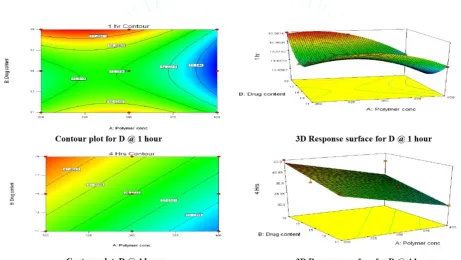
sensitive to the factors as in all cases there is a visible steep slope or curvature in the response plots. After evaluating the perturbation, the factors can now be used to generate 2D contour plots and 3D response surface plots. It can also be reconfirmed from the perturbation plots that D@1 hour and D@ 8 hours are quadratic responses as they show a curve wheres D @ 4 hours and D @ 20 hours show a straight line indicating linearity (in given experimental data). Also a greater curvature and significant slope for the linear response indicate that both factors have impact on each of the responses. The Contour plots for the four responses are plotted in the figures. Each line on the contour represents the same responses at the combination of the two factor levels.

It can be seen that at higher polymer concentrations, and around 13 to 17 % of drug content can help achieve minimum dissolution value at the 1hour time point. Also, at all of the factor combinations, the dissolution does not go beyond the desired limit of 25 % indicating that the chosen factor levels are competent to achieve the desired response. The corresponding 3D response surface for this response is depicted below for better interpretation and visualization of the response surface. It can be observed that the contours for the D @ 4 hours response are linear. It can also be seen that towards lower polymer

concentration (less than 325 mg) and at higher drug % ( greater than 16 %), the dissolution value is above 40 % (as against the desired limit of 20 – 40 %). Hence to be safely inside the limit, one has to choose a higher polymer concentration (greater than 375mg) and lower drug concentration (between 11 to 13 %) to have a lower dissolution value as shown by the 36 % contour at bottom right corner in the above figure. The 3D response surface for this response also helps interpret a linear relationship and the graph is depicted in figure.

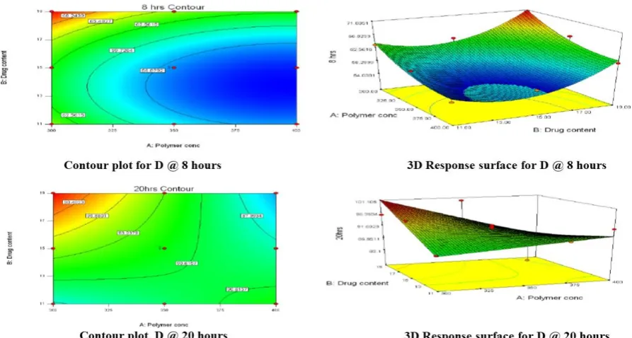
The contour plot for the D @ 8 hours response is again a curvature-based plot indicating higher order terms. The contour indicates desired reponse above 350 mg polymer concentration and between 11 to 15 % drug content. In this plot too, at lower polymer concentration and above 15 % drug content, the dissolution value tends to rise above the spec limit (i.e. 60 %). The contour and the corresponding 3D response surface for D @ 8 hours response is depicted in figures. Although, the response surface is not a good predictor for the response D @ 20 hours, the contour and 3D response surface were constructed to visualize the effect of factors combinations on to the response. This contour plot does not show any pattern (curvature or linearity) with respect to the responses.

(9)

Figure 10: Contour plot with 3D response in 8 hour and 20 hours

OPTIMIZATION:

The optimization module in Design-Expert searches for a combination of factor levels that simultaneously satisfy the requirements placed on each of the responses and factors. It can be only be used when each response has been analyzed independently to establish the appropriate model. Optimization of one response or the simultaneous optimization of multiple responses can be performed

graphically or numerically. Also, one can simultaneously evaluate all the response models for any value of the independent variables using the point prediction node.

Numerical Optimization: The table 8 below compiles the Numerical optimization criteria for each response in order to carry out numerical optimization.

Table 8: Numerical Optimization constraints

Name Goal Lower Limit Upper Limit Weight

Polymer conc Is in range 300 400 3

Drug content Is in range 11 19 3

1 hrs Is in range 10 20 3

The figure 11 below shows the screen shot of possible solutions suggested by the software design expert ® after considering the desired constraints during numerical optimization of the design.

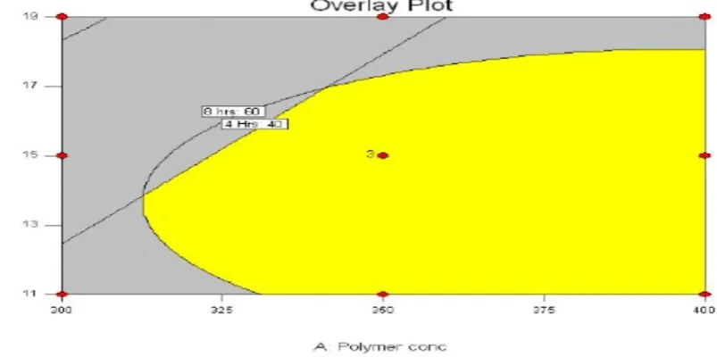
Graphical Optimization: With multiple responses one needs to find regions where critical properties. By superimposing or overlaying critical response contours on a single plot we can visually search for the best combination. When dealing with many input variables, its better to do numerical optimization first, otherwise its impossible to uncover a feasible region. Graphical optimization displays the area of feasible response values in the factor space. Regions that do not fit the optimization criteria are shaded. For multiple responses we may see several overlapping shaded areas. Any "window" that is NOT shaded satisfies the multiple constraints on the responses. The figure 11 depicts the overlaying contours for each response meeting the criteria set in table 8 above The region (yellow) depicts the design space´ for achieving the set of responses with the factor combinations.requirements simultaneously meet the

(10)

Figure 11: Graphical optimization overlay showing the Design Space

Validation of the model: The validation of the model was carried out using the point prediction´ tool in the design expert software. The tool can be used to predict the response by varying the factor combinations. A setting of factors was chosen in the design space and replicated 3 times to

determine the error in predictability of the design and to determine the predicted vs actual variation of the model. The table 9 describes the factor combinations chosen and their predicted vs the actual response.

Table 9: Predicted vs Actual responses

Trial Factor Response Predicted value Actual value _{(Actual –Predicted)}Residual

1

Polymer concentration

(350 mg; Drug Content) 15 %

1 hour 15.1959

15.3 -

- -0.1041

- -

15.2 -0.0041

16 -0.8041

37.5 1.3178

4 hours

38.8178 37.8 1.0178

38.2 0.6178

8 hours 57.3129

56.4 0.9129

57.5 -0.1871

58.4 -1.0871

92 -0.4973

20 hours 91.5027 91.5 0.0027

93.5 -1 .9973

It can be seen that the data of predicted vs actual are in reasonable agreement of each other. Thus, the model can be used to navigate the design space successfully.

SUMMARY AND CONCLUSIONS

The Polyethylene oxide polymers provide a very unique processing advantage over other conventional polymers used in modified release formulation systems. The concentration of the polymer and its grade chosen are the most important factors that affect the formulation design and they have to be chosen based on the desired product performance. The combinations of two viscosity grades do not significantly impact the dissolution of the drug from the system. The use of a high dose highly water-soluble drug presents an added challenge to formulate a modified release dosage form. Initial experiments were carried out to arrive at factors critical to the formulation in order to meet the

(11)

ISSN: 2250-1177 [561] CODEN (USA): JDDTAO statistical models for predicting each of the responses. The

Dissolution at 1 hour and 8 hours followed a quadratic model whereas the models chosen for dissolution at 4 hours and dissolution at 20 hours were estimated a linear and 2FI model respectively. The ANOVA was calculated to determine the significant factors in the model that affect the response outcomes. After fitting of data to the selected models optimization was carried out for achieving the target product profile. The repeatability of the experiments was evaluated by choosing a point in the design space and replicating 3 times to determine the inter response variations and the difference was found to be statistically in-significant. The design of experiments (DOE) approach was thus used to optimize the polyethylene oxide based modified drug delivery system to meet the target product profile for the highly water soluble compound of Metoprolol succinate.

Value addition of this work

The fundamentals and basics of DOE (Design of experiment) learned during this work can be applied to other projects where meeting the desired target product profiles is highly critical. Although, Metoprolol succinate was used as a model drug, the PEO based platform technology can be applied with minor modifications to other compounds with similar properties in order to meet the target specifications. Developing a PEO based modified release drug delivery system can in turn help circumvent the innovator IP and reduce the formulation and process time involved in development thus saving cost and improving throughput responses.

ACKNOWLEDGEMENT

Authors are thankful to SSSUTMS, School of Pharmacy, Sehore and Ipca as well as Alpa laboratories ltd Indore, for providing the necessary facilities & guidance to complete this research.

REFERENCES

1. Regardh G, Borg KO, Johnsson R, Johnsson G and Palmer L, Pharmacokinetic studies on the selective β1-receptor antagonist metoprolol in man, Journal of Pharmacokinetic and Biopharmaceutical, 1974; 2: 347–364.

2. Kendall MJ, Maxwell SR and Westergren SA, Controlled release metoprolol: Clinical pharmacokinetic and therapeutic implications, Clinical Pharmacokinetic, 1991; 5: 319–330. 3. Ragnarsson G, Sandberg A, Jonsson UE and Ggren SJ,

Development of A New Controlled Release Metoprolol Product, Drug Development and Industrial Pharmacy, 1987; 13: 9-11. 4. Dhawan S, M Verma M, and Sinha VR, High Molecular weight

poly (ethyleneoxide) -Based drug delivery system Part 1: Hydrogels and Hydrophilic matrix systems, Pharmaceutical Technology, 2008;12: 72-79.

5. Maggi L, Bruni R, Conte U. High molecular weight polyethylene oxides (PEOs) as an alternative to HPMC in controlled release dosage forms. International Journal of Pharmaceutics 2000; 195: 229-238.

6. Deshkar S, Pawar M, Shirsat A, Shirolkar S. Development of sustained release tablet of Mebeverine hydrochloride. Journal of Pharmaceutical Education & Research, 2013; 4(1): 64-69. 7. Vidyadhara S, Sasidhar RLC, Nagaraju R. Design and

Development of Polyethylene Oxide Based Matrix Tablets for Verapamil Hydrochloride. Indian Journal Pharm Science, 2013; 75(2):185-190.

8. Bukka R, Dwivedi M, Nargund LVG, Prasam K. Formulation and Evaluation of Felodipine Buccal Films containing Polyethylene Oxide. International Journal of Research in Pharmaceutical and Biomedical Sciences. 2012; 3 (3):1153-1158.