New Zealand Journal of Ecology (2005) 29(1): 95-103 ©New Zealand Ecological Society
Forest canopy gap detection and characterisation by the use of
high-resolution Digital Elevation Models
Harley D. Betts
1*, Len J. Brown
1, 2and Glenn H. Stewart
31 Landcare Research (New Zealand) Ltd, Private Bag 11052, Palmerston North, New Zealand. 2 Current address: New Zealand Climate Change Office, PO Box 10362, Wellington, New Zealand. 3 Soil, Plant and Ecological Sciences Division, Lincoln University, PO Box 84, Lincoln, New Zealand.
* Author for correspondence (E-mail: [email protected])
____________________________________________________________________________________________________________________________________
Abstract: The remote identification of forest canopy gaps from Digital Elevation Models (DEMs) built from aerial photographs is potentially a viable alternative to ground-based field surveys. In this study a DEM-based gap-finding algorithm, given suitable experimentally determined input parameters, yielded canopy gap statistics for a study area that were consistent with ground-based survey data from the same area. The method could thus be ‘trained’ to replicate ground-based results for a small test area of beech (Nothofagus) forest, with the potential for it to be applied to larger areas of forest of a similar type to gather canopy gap data with relatively little additional field work. The use of a DEM-based method also has the advantage that the results are easily analysed and mapped using commonly available GIS and cartographic software.
____________________________________________________________________________________________________________________________________
Keywords: Canopy gap; remote detection; Digital Elevation Model; aerial photography; temperate beech forest.
Introduction
The role of disturbances in forest dynamics has been widely recognised (Pickett and White, 1985). In some forests, the disturbance regime is characterized by large, infrequent disturbances with return periods of decades to centuries. Examples include catastrophic fires (Heinselman, 1973), floods (Duncan, 1993), hurricanes (Foster and Boose, 1995), earthquakes (Wells et al., 2001), and volcanic eruptions (Turner et al., 1997). In other forests frequent, less intense disturbances create small-scale openings in the forest canopy so that the forest is constantly turning over and at any one time a significant proportion of the landscape is in a recently disturbed state (Runkle, 1982).
The formation of such small openings in the forest canopy (‘gaps’) was recognised early by Watt (1947). Subsequently, numerous tropical and temperate studies have demonstrated that such treefall gaps are important to the population dynamics of forest trees and to forest composition, structure, and heterogeneity (Brokaw, 1982, 1985a, 1985b; Runkle, 1992; Blackburn and Milton, 1996; Tanaka and Nakashizuka, 1997; Brown and Jennings, 1998; Dube et al., 2001; Ott and Juday, 2002).
However, although it is generally accepted that gaps are important to forest diversity and dynamics, there has been some debate about the recognition of
so-called ‘gaps’ and how they should be appropriately defined and measured (e.g., Lieberman et al., 1989; Runkle, 1992). For example Brokaw (1982) defines a gap (in Panamanian tropical forests) as “… a hole with vertical sides extending through all levels down to an average height of 2 m above the ground”, whereas Nakashizuka et al. (1995) define gaps (in temperate deciduous forests in central Japan) as “…sections of forest canopy lower than 15 m above the ground”. Clearly the definition of a forest canopy gap is somewhat subjective, and also varies according to forest type.
regular line-intersect sampling (Battles et al., 1996), but, while offering improvements over ground surveys in which gaps were defined arbitrarily, such methods still require much time and manual effort, particularly for larger areas (Nakashizuka et al., 1995).
More recently, attempts were made to reduce the effort involved in collecting canopy gap data by means of remote methods—looking at a forest canopy from above instead of from below. Most commercially available satellite imagery, while useful for studying forests at a landscape level (Blackburn and Milton, 1996), is generally too coarse in resolution (i.e., > 5 m per pixel) for the accurate delineation of individual tree crowns. The cost of satellite imagery is also high relative to the small size of most study areas (generally no more than a few tens of hectares, e.g. Tanaka and Nakashizuka, 1997; Fujita et al., 2003). Airborne Laser Scanning (ALS), also known as Light Detection and Ranging (LiDAR), is an emerging remote sensing technology that can accurately estimate forest structure (Lefsky et al., 1999; Lefsky et al., 2002; Lim et al., 2003) and has significant potential for high-resolution identification and mapping of forest canopy gaps. However, the cost of deploying this technology in New Zealand, whilst falling, is currently too high to be cost effective for small study areas.
Aerial photography and airborne digital imagery offer lower cost, alternative sources of high-resolution canopy imagery, and studies on the measurement of canopy gap characteristics from these sources have become more commonplace since the mid-1990s (e.g., Nakashizuka et al., 1995; Tanaka and Nakashizuka, 1997; Fox et al., 2000). However, while suitable for small study sites, the use of manual photogrammetric techniques for mapping canopy structure over large areas is generally not considered cost-effective (Andersen et al., 2003).
More recently, the use of Digital Elevation Models (DEMs) has been investigated as an alternative to ground surveys or intensive manual analyses of aerial photography (e.g., Nakashizuka et al., 1995; Tanaka and Nakashizuka, 1997; Herwitz et al., 1998; Fujita et al., 2003). DEMs are computerised representations of a surface, and can be constructed from a variety of sources including topographic surveys, satellite imagery, aerial photographs and digital airborne imagery. DEMs showing the surface features of a forest canopy can be easily analysed within Geographic Information Systems (GIS) software, making the characterisation of a forest canopy a relatively fast and easy process. This approach has the advantage of being able to rapidly collect data on canopy gap characteristics for extensive areas, with a minimum of field work. It does not, however, allow the collection of additional data such as seedling distributions within gaps.
Nakashizuka et al. (1995) and Tanaka and Nakashizuka (1997) compared DEMs constructed from summer and winter imagery for an area of deciduous forest, and used the apparent elevation differences on the DEMs (relating to the presence or absence of leaves) as an indication of the canopy height. However, New Zealand indigenous forest is not deciduous, so their method could not be used here. Fujita et al. (2003) devised a similar method by which they created a ground DEM from ground measurements and compared it with a DEM of the canopy top created from aerial photographs. This approach, whilst useful for evergreen forests where a ground DEM cannot be created from winter photography, still requires researchers to visit almost their entire study site on foot to acquire ground data.
Our study describes the use of a semi-automated method, based on a high-resolution DEM constructed from scanned aerial photographs, to identify and characterise canopy gaps in an area of indigenous temperate beech (Nothofagus spp.) forest on New Zealand’s South Island. Forest canopy gaps were identified, mapped and measured using an algorithm that compared the elevation of the interiors of gaps with the elevation of a “canopy top” surface that was interpolated from the surrounding forest canopy. The results in this study were obtained by “training” the algorithm to replicate a target set of canopy gap data for the same study site that was obtained from a previous ground survey (Stewart et al., 1991). The method is still in its infancy; however, it does have the potential advantage of being able to be applied to larger areas of the same forest type, once it has successfully replicated a target set of data, without need for the entire site to be visited on the ground.
Methods
Study area
Figure 1. Location of the study site adjacent to an access road in the Maruia Valley, northwestern South Island, New Zealand.
large-diameter N. fusca, up to 30 m tall, over smaller diameter N. menziesii, which have a maximum height of approximately 25 m (Runkle et al., 1995). Understorey vegetation at the site is sparse (Stewart et al., 1991). Fifty canopy gaps were identified and measured at the site in 1987 by Stewart et al. (1991), and 48 of these fell inside the study area delineated on the DEMs used in this study.
Aerial photography and DEM construction
The earliest available aerial photography suitable for this study was taken in January 1990. We used a single stereopair which provided colour infrared stereo coverage of the site at a scale of 1:15 000; these were scanned at 12.5 µm to produce high-resolution digital imagery with a ground resolution of 0.19 m per pixel. The software used to generate the DEM used in this study was IMAGINE OrthoMAX Version 8.2, a softcopy terrain mapping and geopositioning package developed by Vision International (ERDAS Incorporated, Georgia, USA, 1992). For a DEM to be generated from stereo imagery, OrthoMAX required each image to contain a number of points of known position and elevation. Ground control points used in this study were surveyed by a differentially corrected
Global Positioning System (GPS) to a nominal precision of 1.5 m. A minimum of four control points per image were collected, using widely dispersed and readily identifiable features in the field such as road intersections, logs on the roadside, and points where roads crossed over streams. These points, in conjunction with details of the geometry of the camera and lens used for the photography, were then used by OrthoMAX to calculate, by triangulation, the camera position and attitude for each image.
The calculated camera positional data were then used to build the DEM for the study site by stereo-matching features present in both images, calculating the elevation for the entire study site point-by-point based on the degree of relief displacement from one image to the next. ERDAS Incorporated advise that the best results are gained when a DEM is generated at a resolution of approximately one-fifth of that of the original imagery; therefore, with a ground pixel resolution of 0.19 m in our original imagery, we generated our DEM at a resolution of 1.0 m.
The quality of the matching process depends, in part, on the textural quality of the original images (Betts and De Rose, 1999). At any point where the images lack sufficient texture to allow a successful match, the matching algorithm fails and the elevation for that point is then estimated (interpolated) from neighbouring points. The accurate representation of canopy gaps on a DEM can be adversely affected by interpolation, as gap interiors tend to be in shadow on the original imagery and therefore often have
insufficient textural definition for successful pixel matching in OrthoMAX.
Canopy gap detection
The process of gap detection from the forest canopy DEM is summarised in Figure 2. The method first required the construction of a canopy top DEM, in which a local maximum filter and then a smoothing (local mean) filter were applied to the forest canopy DEM to create a new surface that approximated the level of the top of the forest canopy. The filters, essentially square roving windows of a specified size (in pixels), calculated a new elevation value for the pixel at the centre of each window location based on the elevation values of the surrounding pixels within the window. By way of example, using our 1-m resolution DEM, a 15×15 pixel local maximum filter was a roving window of 15 m on a side; when it was applied to the DEM it gave to the centre pixel for each location the maximum elevation value encountered within 7 m (the distance from the centre pixel to the edge of the roving window) of that centre pixel. The window was then moved by one pixel and the calculation repeated, and so on, until the window had been applied to the whole DEM, pixel by pixel. In other words, the canopy top DEM was derived for the original DEM such that, for any point on the original DEM, the canopy top DEM contained the highest elevation (pixel value) that occurred on the original DEM within 7 m of that point. The canopy top DEM can therefore be likened to a surface that could be obtained by stretching an imaginary blanket over the original canopy surface.
The filter size was initially chosen to be just larger in area than the largest gap measured in the ground survey. This ensured the canopy top DEM did not include lower elevations from within canopy gaps, and therefore cause the algorithm to underestimate or fail to detect some gaps. Further testing showed that a filter of size about 30% larger than the largest gap recorded on the ground yielded the best results, as discussed below.
Following construction of the canopy top DEM, the elevations in the original DEM were then subtracted from those in the canopy top DEM to create a difference image. Elevation differences in the difference greater than a threshold value were provisionally taken to represent canopy gaps (Fig. 3).
The difference image was then converted to a polygon file, in Arc/Info Version 8.1 (ESRI Corporation, California, U.S.A.), for analysis. The process of converting the gaps to polygons assigns each gap a unique identity, and also assigns attributes containing information on gap area and perimeter for each gap. This makes it very easy to select gaps and perform calculations based on their attributes.
Small gaps (of area less than 20 m2) were not recorded in the ground survey on which this study is based, and, therefore, were similarly removed from the DEM-derived data set. The ground survey also excluded highly elongated or irregular gaps that were narrower than 5 m on a side, irrespective of gap area, on the premise that they were not significantly influential on seedling performance on the ground. A useful statistic for removing small, highly irregular gaps is the ratio between a gap’s area and its perimeter, a ratio that decreases with increasing irregularity and decreasing size. Therefore, for the DEM method, small, irregular gaps were removed on the basis of their area:perimeter ratios being below a certain threshold value. Island polygons (polygons occurring within polygons) were manually deleted, on the basis that they were likely to represent one or more isolated trees within a gap that, while still being lower than the forest canopy, were still sufficiently high to affect the canopy top DEM within a gap (during the ground survey, isolated trees within gaps were similarly ignored).
The threshold values for the size of the filter window, the elevation differences taken to represent a gap, and the area:perimeter ratio used to remove small, narrow gaps, were determined iteratively by trial and error such that the final gap data statistics were similar to those gained by the ground survey. The sensitivity of the results to these three parameters is discussed below.
Results
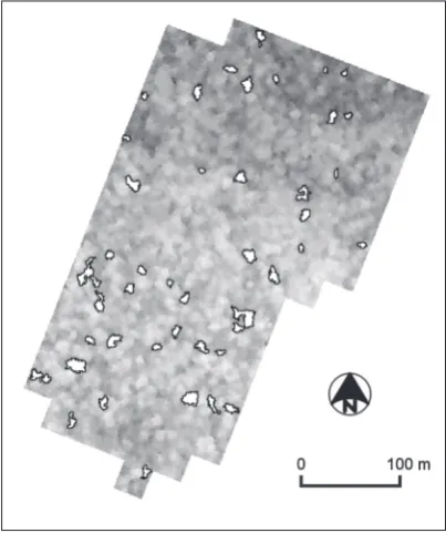
Figure 4. Canopy gaps in the study site as estimated from the DEM. The grey tones in the DEM are directly proportional to elevation (lighter tones have higher elevation); DEM-derived canopy gaps are shown as white areas outlined in black.
Figure 5. The effect on the DEM-derived results of varying the three main parameters used in the model: (A) Depth below canopy top DEM; (B) Width of search window; (C) Area-to-perimeter ratio.
Table 1. Ground survey-based gap data and DEM-based gap data for the study site.
____________________________________________________________________________________________________________________________________
Number Mean gap Median gap Standard Maximum Minimum
of gaps area (m2) area (m2) deviation gap area gap area
of gap area (m2) (m2)
(m2)
____________________________________________________________________________________________________________________________________
Ground-based data 48 79.7 69.2 40.5 200.2 23.6
DEM-based data 46 76.2 65.0 46.5 224.0 20.0
____________________________________________________________________________________________________________________________________
variability in canopy-gap size as measured by the DEM was slightly greater than measured on the ground, although the total number of gaps and the mean and median gap size figures agreed well.
Three main parameters controlled the results obtained in this study (summarised in Fig. 5). First, DEM gap statistics were affected by the vertical elevation difference between the canopy top and original DEMs that was taken to constitute a gap (Fig. 5A). Canopy gaps were generally represented by deep, steep-sided depressions on the DEM, with variable side slope angles. Therefore, the abundance and size of gaps as detected by the DEM method were strongly influenced by the value of the elevation difference that was interpreted to be a canopy gap. A large difference
(e.g. 16 m) resulted in underestimates of gap statistics, while a small difference (e.g. 8 m) led to overestimates. In the ground survey, a gap was taken to be a drop of 10 m or more from the surrounding canopy, while a drop of 12 m yielded the best results from the DEM method.
leading to the interpretation of topographic hollows or local variations in canopy height as large canopy gaps, and, consequently, overestimates of canopy gap size and abundance. Small filters thus tended to result in small gaps and large filters returned large gaps. A filter size of 17×17 m, approximately 30% larger in area than the largest gap recorded on the ground, was found to be optimal. This represented a tradeoff between the risk of allowing the canopy top DEM to fall into gaps by using too small a filter, and the tendency of large filters to over-generalise the canopy top.
Third, gap statistics were influenced by the chosen threshold value for the area:perimeter ratio, which was used to accept or discard small and/or very irregular gaps (Fig. 5C). This ratio is low for very small and/or irregular gaps, and increases with gap size and decreasing irregularity. A low threshold led to more gaps being retained in the sample, while raising the threshold reduced the sample in favour of large, less irregular gaps.
Discussion
These results clearly demonstrate the need for the DEM method to be trained to replicate a trial set of ground-based survey data, by experimentally varying each of these three parameters in turn. Once this training is successful (that is, a sample set of ground-based gap data has been closely replicated by the DEM method), this method can then be used to quickly gather data on canopy gaps over larger areas of the same forest type for relatively little additional effort. An advantage of this method is that it is designed to work on evergreen forests where there is little or no opportunity for aerial photographic surveys of the underlying ground surface. Because it is based on analysing a single DEM of the forest canopy, there is no requirement for a second DEM of the underlying ground surface to compare it with (e.g. Nakashizuka et al., 1995; Tanaka and Nakashizuka, 1997; Fujita et al., 2003). This means, for the method to be used, only one photographic survey and one field trip (to establish a test set of ground gap data and set up ground control points) would be needed.
This method would also enable researchers to map changes accurately and objectively in a forest canopy over time, using repeat photography taken to the same specifications each time and based on the same set of ground control points (e.g. Herwitz et al., 1998). Once a digital dataset of canopy gaps has been produced, it would also be a relatively simple process to use this in a GIS software package to calculate other spatial characteristics of forest canopy gaps such as gap density, percentage of forest area in gaps, gap shape, gap spacing, dispersion index for gaps, and gap spacing
statistics (Blackburn and Milton, 1996). In contrast, to calculate the same attributes manually from a ground-based survey would be a very time-consuming task, especially for a large area. Having a gaps map already in digital form also means it is easy to produce hardcopy maps of canopy gaps and their attributes if required, using various cartographic facilities now commonly available within most GIS software packages.
As well as enabling the rapid collection of gap data over relatively large study sites, the DEM method also offers efficiencies in modelling applications because the data are available in high-resolution digital form that can be easily manipulated using a range of cartographic and GIS software packages. For example, the ability to produce a high-resolution DEM of a forest canopy, together with an accurate map of gap locations and characteristics, would enable researchers concerned with seedling performance within gaps to model light environments at the forest floor by using these data layers together with available information on sun angle and cloud cover.
Whilst offering a number of advantages over manual gap surveying methods and many remote methods, the DEM method also has some limitations. For example, the DEM method has been developed on an almost flat site, whereas much of New Zealand’s topography is mountainous. Further testing would therefore be required to test the robustness of the method with respect to variations in topography. The current study has also been carried out on a relatively simple, uniform forest type, dominated by only two canopy species. However forest canopy morphology is often highly variable, particularly for mixed podocarp-hardwood forests or where widespread natural or anthropogenic disturbance has occurred, and therefore the DEM method will probably need to be modified to yield acceptable results in these situations. In particular, a forest characterised by tall emergent trees within a matrix of shorter species would probably require a modified version of the method due to its reliance on comparisons of the canopy elevation at a point with the maximum height of the surrounding canopy (which would be confounded by the presence of emergent trees). Very large gaps or areas of major disturbance may also be problematic because of the canopy top DEM’s tendency to descend to the floor of very large gaps and therefore lead to underestimates in overall gap statistics. This is especially challenging where the range in gap sizes is very large, because if a filter size is chosen to cope with the largest gaps it may lead to overestimates of smaller gaps within the same study area.
OrthoMAX and other texturally based image matching algorithms, the process of DEM construction from aerial photography relies on the original images containing sufficient texture for features to be matched between images. Areas of low textural definition, such as within shadows, are usually poorly represented on DEMs built from aerial photography in this way. This presents a problem for gap studies in particular because canopy gap interiors are usually shaded by the surrounding canopy. As mentioned above, wherever image matching in OrthoMAX fails, the elevation of that point is instead interpolated from surrounding successfully matched points. Interpolation, therefore, reduces the size and number of gaps detected by the DEM method because it tends to fill the gaps on the forest canopy DEM.
Because it is based on aerial photography, the effects of sun angle on the degree of shading within gaps (and consequent interpolation during DEM construction) may be especially problematic for winter images. Either the method would need to be modified to accommodate excessive shadowing, or else be limited to using summer photography only. Bad weather conditions may also delay the acquisition of aerial photography.
The recent development of LiDAR offers an attractive alternative means of acquiring high-resolution canopy DEM data (Lefsky et al., 1999; Lefsky et al., 2002). Because LiDAR uses active laser and therefore does not rely on illumination by natural sunlight (Shrestha et al., 2000), LiDAR-based aerial surveys can be carried out at short notice at any time of year, and data can be collected by day, by night, or in shadowed areas (Renslow and Gross, 2001). The main drawbacks with using LiDAR in New Zealand are its present high cost, and the relative paucity of operators that offer this technology. However, as the technology improves and the cost declines, it is expected that LiDAR will become more widely offered and used in the near future. Until this occurs, however, LiDAR is generally regarded as being too expensive to commission, especially for most small studies (Renslow and Gross, 2001).
Conclusions
The use of a high-resolution DEM to identify and map forest canopy gaps has shown positive results, demonstrating that the method has merit as a means for rapidly acquiring information on canopy gaps for considerably less effort than would be required if the same data was gained by manual field measurements. The results gained by the DEM method are sensitive to individual site characteristics, and therefore the method needs to be trained to replicate a small sample set of
ground-based data before it can be applied to a larger area of the same forest type. This training is achieved by experimentally varying the three main parameters (canopy gap threshold depth, search window size and gap area:perimeter ratio) on which the method is based, until the results so gained give a close match to the control data set. While initial results are promising, further work is needed to investigate the robustness of this method, particularly with respect to topography and forest composition and structure.
Acknowledgements
We would like to thank Pamela Brown, Larry Burrows and Ted Pinkney for field assistance and advice. We would also like to thank Peter Bellingham, Heather North and Rob Allen and two anonymous referees for comments on drafts of this manuscript. This study was funded by the Foundation for Research Science and Technology, Contract No. CO9X0006.
References
Andersen, H.; McGaughey, R.J.; Carson, W.W.; Reutebuch, S.E.; Mercer, B.M.; Allan, J. 2003. A comparison of forest canopy models derived from LIDAR and INSAR data in a Pacific Northwest conifer forest. In: Maas, H.-G.; Vosselman, G.; Streilen, A. (Editors), Proceedings of the International Society of Photogrammetry and Remote Sensing (ISPRS) Working Group III/3 Workshop “3-D Reconstruction From Airborne Laserscanner and InSAR Data”. Institute of Photogrammetric Engineering and Remote Sensing, Dresden, Germany, 8-10 October 2003. URL: http://www.isprs.org/commission3/wg3/ w o r k s h o p _ l a s e r s c a n n i n g / p a p e r s / Andersen_ALSDD2003.pdf. Accessed 30 April 2004.
Battles, J.J.; Dushoff, J.G.; Fahey, T.J. 1996. Line intersect sampling of forest canopy gaps. Journal of Forest Science 42:131-138.
Betts, H.D.; De Rose, R.C. 1999. Digital Elevation Models as a tool for monitoring and measuring gully erosion. Journal of Applied Earth Observation and Geoinformation 1: 91-101. Blackburn, G.A.; Milton, E.J. 1996. Filling the gaps:
remote sensing meets woodland ecology. Global Ecology and Biogeography Letters 5: 175-191. Bartemucci, P.; Coates, K.D.; Harper, K.A; Wright, E.
2002. Gap disturbances in northern old-growth forests of British Columbia, Canada. Journal of Vegetation Science 13: 685-696.
Geological map of New Zealand 1:250 000. Department of Scientific and Industrial Research, Wellington, N.Z.
Brokaw, N.V.L. 1982. The definition of treefall gap and its effect on measures of forest dynamics. Biotropica 14: 158-160.
Brokaw, N.V.L. 1985a. Gap-phase regeneration in a tropical forest. Ecology 66: 682-687.
Brokaw, N.V.L. 1985b. Treefalls, regrowth, and community structure in tropical forests. In: Pickett, S.T.A.; White, P.S. (Editors), The ecology of natural disturbance and patch dynamics, pp. 53-69. Academic Press, New York, U.S.A. 472 pp. Brokaw, N.V.L.; Grear, J.S. 1991. Forest structure
before and after Hurricane Hugo at three elevations in the Liquillo Mountains, Puerto Rico. Biotropica 23: 386-392.
Brown, N.D.; Jennings, S. 1998. Gap-size differentiation by tropical rain forest trees: a testable hypothesis or a broken-down bandwagon? In: Newbery, D.M.; Prins, H.H.T.; Brown, N.D. (Editors), Dynamics of tropical communities, pp. 79-94. Blackwell, Oxford, U.K. 635 pp. Dube, P.; Fortin, M.J.; Canham, C.D.; Marceau, D.J.
2001. Quantifying canopy gap dynamics at the patch mosaic level using a spatially-explicit model of a northern hardwood forest ecosystem. Ecological modelling 142: 39-60.
Duncan, R.P. 1993. Flood disturbance and the coexistence of species in a lowland podocarp forest, south Westland, New Zealand. Journal of Ecology 81: 403-416.
ERDAS® Incorporated. 1992. IMAGINE OrthoMAX™ User’s Guide. ERDAS®, Incorporated, Atlanta, GA 30329, U.S.A.
Foster, D.R.; Boose, E.R. 1995. Hurricane disturbance regimes in temperate and tropical forest ecosystems. In: Coutts, M.; Grace, J. (Editors), Wind and Trees, pp. 305-339. Cambridge University Press, Cambridge, U.K. 501 pp. Fujita, T.; Itaya, A.; Miura, M.; Manabe, T.; Yamamoto,
S. 2003. Long-term canopy dynamics analysed by aerial photographs in a temperate old-growth evergreen broad-leaved forest. Journal of Ecology 91: 686-693.
Fox, T.J.; Knutson, M.G.; Hines, R.K. 2000. Mapping forest canopy gaps using air-photo interpretation and ground surveys. Wildlife Society Bulletin 28: 882-889.
Heinselman, M.L. 1973. Fire in the virgin forests of the Boundary Waters Canoe area, Minnesota. Quaternary Research 3: 329-382.
Herwitz, S.R.; Slye, R.E.; Turton, S.M. 1998. Co-registered aerial stereopairs from low-flying aircraft for the analysis of long-term tropical rainforest dynamics. Photogrammetric
Engineering and Remote Sensing 64: 397-405. Lefsky, M.A.; Cohen, W.B.; Acker, S.A.; Parker,
G.G.; Spies, T.A.; Harding, D. 1999. Lidar remote sensing of the canopy structure and biophysican properties of Douglas-fir western Hemlock forests. Remote Sensing of Environment 70: 339-361. Lefsky, M.A.; Cohen, W.B.; Parker, G.G.; Harding,
D.J. 2002. Lidar remote sensing for ecosystem studies. BioScience 52: 19-30.
Lieberman, M.; Lieberman, D.; Peralta, R. 1989. Forests are not just Swiss cheese: canopy stereogeometry of non-gaps in tropical forests. Ecology 70: 550-552.
Lim, K.; Treitz, P.; Baldwin, K.; Morrison, I.; Green, T. 2003. Lidar remote sensing of biophysical properties of tolerant northern hardwood forests. Canadian Journal of Remote Sensing 29: 658-678.
Nakashizuka, T.; Katsuki, T.; Tanaka, H. 1995. Forest canopy structure analysed by using aerial photographs. Ecological Research 10: 13-18. Ott, R.A.; Juday, G.P. 2002. Canopy gap characteristics
and their implications for management in the temperate rainforests of southeast Alaska. Forest Ecology and Management 159: 271-291. Pickett, S.T.A.; White, P.S. 1985. The Ecology of
Natural Disturbances and Patch Dynamics. Academic Press, New York, U.S.A. 472 pp. Renslow, M.S.; Gross, S.B. 2001. Technology
assessment of remote sensing applications: LIDAR. National Consortium for Safety, Hazards and Disaster Assessment of Transportation Lifelines Technical Notes 6. U.S. Department of Transportation National Consortia on Remote Sensing in Transportation, University of New Mexico, NM 87131-6031, U.S.A. URL: http:// r i k e r . u n m . e d u / D A S H _ n e w / p d f / Technical%20Notes/LIDAR.PDF. Accessed 18 April 2004.
Runkle, J.R. 1982. Patterns of disturbance in some old-growth mesic forests of eastern North America. Ecology 63: 1533-1546.
Runkle, J.R. 1992. Guidelines and sample protocol for sampling forest gaps. General technical report, PNW-GTR-283, USDA Forest Service. Pacific Northwest Research Station, Portland, Oregon, U.S.A. 44 pp.
Runkle, J.R.; Stewart, G.H.; Veblen T.T. 1995. Sapling diameter in gaps for two Nothofagus species in New Zealand. Ecology 76: 2107-2117.
h t t p : / / w w w . a l s m . u f l . e d u / p u b s / a c c u r a c y / accuracy.htm. Accessed 24 March 2004. Stewart, G.H.; Rose, A.B.; Veblen, T.T. 1991. Forest
development in canopy gaps in old-growth beech (Nothofagus) forests, New Zealand. Journal of Vegetation Science 2: 679-690.
Tanaka, H.; Nakashizuka, T. 1997. Fifteen years of canopy dynamics analyzed by aerial photographs in a temperate deciduous forest, Japan. Ecology 78: 612-620.
Turner, M.G.; Dale, V.H.; Everham, E.H. 1997. Fires, hurricanes, and volcanoes: comparing large disturbances. BioScience 47: 758-768.
Watt, A.S. 1947. Pattern and process in the plant community. Ecology 35: 1-22.
Wells, A.; Duncan, R.P.; Stewart, G.H. 2001. Forest dynamics in Westland, New Zealand: the importance of large, infrequent earthquake-induced disturbance. Journal of Ecology 89: 1006-1018.