Tsunami waveform inversion by numerical finite-elements
Green’s functions
A. Piatanesi, S. Tinti, and G. Pagnoni
Dipartimento di Fisica, Universit`a di Bologna, Bologna, Italy Received: 06 August 2001 – Accepted: 16 November 2001
Abstract. During the last few years, the steady increase in the quantity and quality of the data concerning tsunamis has led to an increasing interest in the inversion problem for tsunami data. This work addresses the usually ill-posed prob-lem of the hydrodynamical inversion of tsunami tide-gage records to infer the initial sea perturbation. We use an in-version method for which the data space consists of a given number of waveforms and the model parameter space is rep-resented by the values of the initial water elevation field at a given number of points. The forward model, i.e. the calcu-lation of the synthetic tide-gage records from an initial water elevation field, is based on the linear shallow water equations and is simply solved by applying the appropriate Green’s functions to the known initial state. The inversion of tide-gage records to determine the initial state results in the least square inversion of a rectangular system of linear equations. When the inversions are unconstrained, we found that in or-der to attain good results, the dimension of the data space has to be much larger than that of the model space parameter. We also show that a large number of waveforms is not sufficient to ensure a good inversion if the corresponding stations do not have a good azimuthal coverage with respect to source directivity. To improve the inversions we use the available a priori information on the source, generally coming from the inversion of seismological data. In this paper we show how to implement very common information about a tsunamigenic seismic source, i.e. the earthquake source region, as a set of spatial constraints. The results are very satisfactory, since even a rough localisation of the source enables us to invert correctly the initial elevation field.
1 Introduction
In the last few years, a great effort has been made to improve the quantity and the quality of the collected data concerning tsunamis. An example is the Deep-ocean Assessment and Correspondence to: A. Piatanesi ([email protected])
Reporting of Tsunami (DART) system for tsunami detection and forecasting, build-up by the Pacific Marine Environmen-tal Laboratory/NOAA (USA) (Titov et al., 1999). Today, any relevant tsunami occurring in the Pacific area is recorded at several tide-gage stations distributed along the coastline of many countries facing the Pacific Ocean. Just to give an ex-ample we can mention the last tsunami generated near the coast of Peru on 23 June 2001, for which some tens of good tide-gage and ocean bottom pressure gage records have been made available to the scientific community with a time lag of only one day. For those tsunamis that cause deaths and large coastal inundation, in addition to these “far-field” data, local data are collected: actually, it is now a standard practice to organize a post-event field survey with the purpose of mea-suring run-up heights along the most affected segments of coast, in order to obtain a detailed picture of the inundation scenario.
Fig. 1. Water elevation field representing the initial conditionζ (t0).
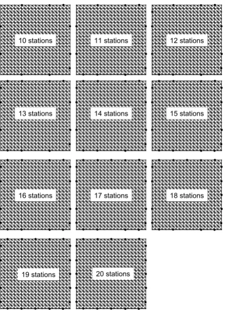
20 stations 19 stations
18 stations 17 stations
16 stations
15 stations 14 stations
13 stations
12 stations 11 stations
10 stations
Fig. 2. Station distributions relative to the inversion experiments where various number of waveforms are used.
Very recently, Pires and Miranda (2001) proposed an ad-joint method for tsunami waveform inversion, as an alterna-tive to the technique based on Green’s functions of the linear long wave model (Satake, 1987). In the present paper we use an inversion method, already described in its fundamentals in a previous paper (Tinti et al., 1996), for which the data space consists of a given number of tide-gage records and
Fig. 3. Dependence of the misfit on the number of waveforms con-sidered in the inversions.The corresponding station distributions are sketched in Fig. 2.
the model parameter space is represented by the values of the initial water elevation field at a given number of points. One of the main advantages of this method is that it does not require an a priori assumption of a fault plane solution: ac-tually, as we will see in the following section, this method is completely independent of any particular source model.
2 Inversion method
The forward model for the tsunami propagation, i.e. for the calculation of the synthetic tide-gage records starting from an initial water elevation field, is based on the linear shallow water equations:
∂tζ = −∇ ·(hv)
∂tv= −g∇ζ , (1)
completed by the following boundary conditions: v·n=g
cζ on the open boundary (2a)
v·n=0 on the solid boundary. (2b)
In the above equations ζ is the water elevation above the mean sea level, v = (u, v) is the horizontal fluid veloc-ity vector whose x- and y-components are, respectively, u and v, h is the basin depth, g is the gravity acceleration, c =(gh)1/2is the wave phase speed andnis the unit vec-tor, outwardly directed, normal to the boundary. To solve Eqs. (1) and (2) we use a finite-element technique: as shown in Tinti and Piatanesi (1995), finite-element spatial discreti-sation transforms Eqs. (1) and (2) into a linear set of ordinary differential equations that are first order in time and that can be put in the following compact form:
d
Fig. 4. Initial fields inverted using 10, 12 and 16 waveforms.
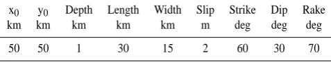
Table 1. Fault parameters of the seismic source used to compute the initial condition
x0 y0 Depth Length Width Slip Strike Dip Rake
km km km km km m deg deg deg
50 50 1 30 15 2 60 30 70
Here,ξ =(ζ, u, v)is a 3N-components vector representing the value of the unknown fields on the nodes of the finite-element grid consisting of N nodes and A is a matrix of con-stant coefficients that also includes the boundary conditions (see Tinti and Piatanesi, 1995). The classical theory of the linear set of differential equations (e.g. Arnold, 1978) pro-vides a formal solution for the unknown vectorξ(t )of Eq. (3) through a spectral decomposition of the matrix A:
ξ(tk)=exp [A(tk−t0)]ξ(t0)=
Eexp [3(tk−t0)] E−1ξ(t0), (4) whereξ(tk)is the unknown vector computed at the timetk, E and E−1are, respectively, the eigenvectors matrix and its inverse, whereas3 is the diagonal eigenvalues matrix and ξ(t0)is the initial condition. From Eq. (4) we can define the Green’s function of the problem as:
Gikj =Einexp [3nm(tk−t0)]Emj−1, (5) where the rule of summation on the repeated index is adopted. If we restrict the problem to the case of a static initial condition and to the calculation of the water elevation ζ (t )solely, the forward problem can be written in terms of the Green’s functions as:
ζi(tk)=Gikjζj(t0). (6) In Eq. (6),ζi(tk)is the elevation computed at thei-th node at the timetk and the Green’s function Gikj has the usual interpretation as the elevation on the nodei at the time tk, produced by a unitaryδ-shapeζ pulse applied on the nodej at the timet0.
As already stated, our inverse problem consists of provid-ing a given number of tide-gage records as data input to ob-tain the initial water elevation fieldζj(t0)as output. Let us
denote byN the number of grid nodes, byRthe number of the available tide-gage records and byP the number of data points on each record: the system consisting ofR×P equa-tions and theN unknownsζj(t0)(j = 1, ..., N )that math-ematically represents our inverse problem can be written in the following way:
ζ1(t1)=G11ζj(t0)
.. .
ζ1(tP)=G1Pjζj(t0)
..
. (7)
ζN(t1)=GN1jζj(t0)s
.. .
ζ1(tP)=GNPjζj(t0)
.
Since the number of rows is greater or equal to the number of columns (R×P ≥ N), the solutionζj(t0)will be com-puted through a least square inversion of the system (7). In the following sections we will illustrate a series of numerical experiments performed on synthetic tide-gage records that will enable us to point out the main features of the proposed inversion method.
3 Inversion experiment set-up
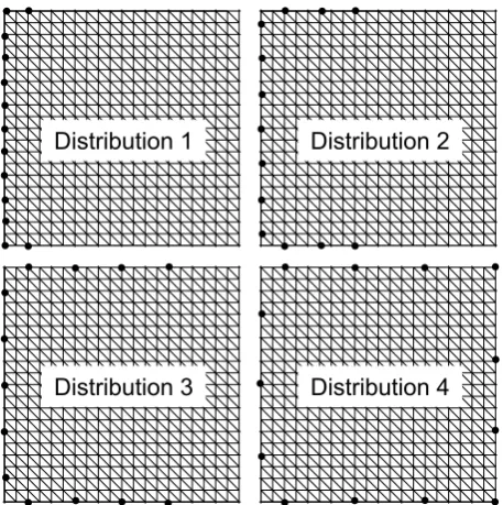
Distribution 1
Distribution 2
Distribution 3
Distribution 4
Fig. 5. Station distributions with different azimuthal coverage of the domain.
by1t the sampling interval on a record,P can be obviously expressed as:
P= Tend
1t . (8)
We choose a sampling interval1t = 60 s that represents a common value for most tide-gages installed to record tsunami waveforms; since in our simulations we consider Tend = 6000 s, each synthetic record will have a number of pointsP =100.
As the initial conditionζ (t0), we consider the coseismic vertical displacement of the sea bottom produced by a seis-mic fault that we compute through Okada’s analytical model (Okada, 1992): the fault parameters are listed in Table 1, while the corresponding water elevation field is shown in Fig. 1.
With the above initial condition and using the computed Green’s functions, we build up the data space, consisting of the synthetic tide-gage records computed by means of Eq. (6) at virtual stations located on the nodes belonging to the boundary. To estimate the goodness of an inversion ex-periment we use anL2-norm misfit parameter that represents the squared averaged difference between the theoretical ini-tial fieldζt heand the inverted oneζinv:
ε= " P
i ζit he−ζ inv i
2
P
i ζit he
2 #
1 2
i=1, ...,N. (9)
Since real tsunami tide-gage records are always affected by errors, we take into account such uncertainty in the data by injecting a Gaussian random noise of 10% in magnitude into the synthetic waveforms. As we will see in the next section, where the results of the inversions experiments are presented,
Fig. 6. Dependence of the misfit on the type of stations distribution (sketched in Fig. 5).
this will give us the opportunity to estimate the robustness of the inversion with respect to fluctuations in the data, in terms of the variance reduction of the misfit parameter.
4 Unconstrained inversion experiments
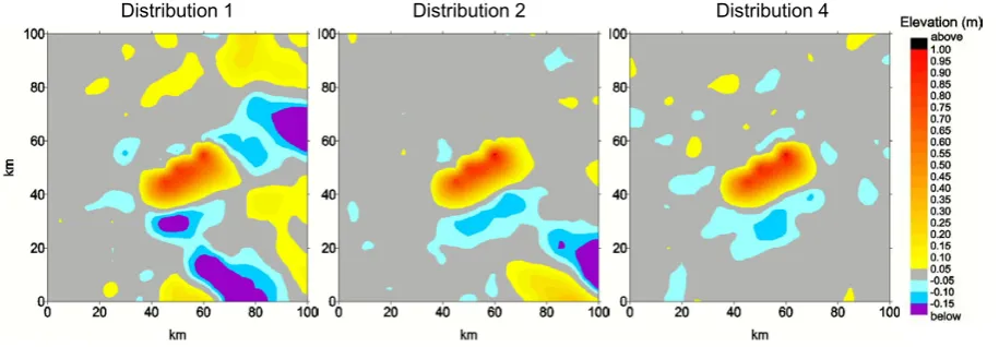
Fig. 7. Representative initial fields inverted using different stations distributions (shown in Fig. 5).
Constraint 1
Constraint 2
Constraint 4
Constraint 3
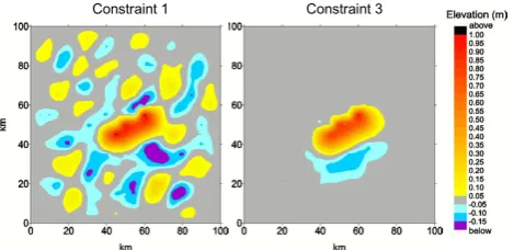
Fig. 8. Sketch of the spatial constraints used to improve the inver-sions with 10 waveforms: the initial field is taken equal to zero in the shaded zones.
fields inverted using a growing number of records. The inver-sion performed with 10 stations leads to an initial elevation field completely different from the theoretical one (see Fig. 1 for comparison): it is characterised by large and uncorrelated wave amplitudes that are indicative of an unstable inversion. The initial field inverted with 12 stations, corresponding to a misfit of 0.36, is visibly closer to the correct shape: the main positive-negative wave system, located in the middle of the basin, is reproduced in its main features, whereas several patches of noise are still present. Finally, when the inversion is performed with 16 waveforms, the inverted field is very close to the theoretical one: both the shape and the ampli-tude are well reproduced and the elevation field is noiseless. The number of records is only one of the parameters that
Fig. 9. Dependence of the misfit on the spatial constraints shown in Fig. 8.
Constraint 1 Constraint 3
Fig. 10. Representative initial fields inverted by using 10 wave-forms and applying the constraints shown in Fig. 8.
Constraint 1
Constraint 2
Constraint 3
Constraint 4
Fig. 11. Sketch of the spatial constraints used to improve the in-versions with the station distribution of type 1, characterised by the lowest azimuthal coverage: the initial field is taken to be equal to zero in the shaded zones.
very low there. This feature does not appear in the case of distribution 4, characterised by an uniform azimuthal cover-age.
5 A priori information: spatial constraints
In all the numerical experiments carried out until now, we have made the explicit assumption that the inversion is un-constrained, so that the degrees of freedom of the problem are equal toN, i.e. to the number of the grid nodes where we look for the solution. Anyway, for the kind of problem we are dealing with, i.e. the inversion of the displacement field induced by a tsunamigenic seismic source, this is an unlikely work condition. From the inversion of seismological data, in most cases we have at least some knowledge about the source location that enables us to look for the solution only in a
re-Fig. 12. Dependence of the misfit on the spatial constraints shown in Fig. 11.
stricted region of the domain: this represents a type of the so-called a priori information. In our inverse modeling this type of a priori information can be easily implemented as a set of spatial constraints: more precisely, the elevation on the nodal points belonging to regions where we have not looked for the solution are set equal to zero. As we will show in the following, the use of the a priori information reduces the di-mension of the model space parameters, leading, in general, to better solutions. We also present an example to show that this kind of constraint should be used with some prudence. 5.1 Constraints improving the solution
To show the improvement of the inversion due to the applica-tion of the spatial constraints, we consider two cases, already discussed in Sect. 4, for which the unconstrained inversion leads to bad results. The first case is the inversion performed using 10 stations: assuming that the initial field is confined in the middle of the basin, we apply constraints that are pro-gressively stronger, setting to zero the water elevation on the nodes belonging to the grey shaded regions, shown in Fig. 8. The application of the constraint of type 1 reduces the model space dimension from N = 441 to N = 361 (∼18% of reduction) and leads to a misfit reduction by a factor 6 (see Fig. 9): we may appreciate, in Fig. 10, that now the corre-sponding inverted initial field shows the main positive wave patch, even if the field is still largely noisy. As shown in Fig. 9 and in Fig. 10, running the inversion with even stronger constraints, rapidly leads to very good results, qualitatively equivalent to those obtained using a much larger number of waveforms (see Figs. 3 and 4 for comparison).
Fig. 13. Representative initial fields inverted by using the stations distribution of type 1 and applying the constraints shown in Fig. 11.
Constraint 1 Constraint 12
Fig. 14. Sketch of progressively stronger constraints: the initial field is taken to be equal to zero in the shaded zones. The theoretical initial elevation field is also shown.
inversion more robust, also leading to a consistent misfit re-duction (see Fig. 12). As shown in Fig. 13, even with a bad distribution of stations, we are able to correctly recover the initial elevation field (see Fig. 7 for comparison).
5.2 An example of bad constraints
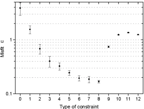
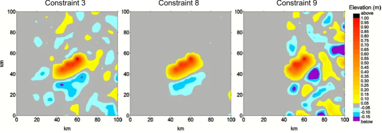
We have seen, until now, that the application of the spatial constraints had always led to improved solutions. Here, we show that the use of a constraint that is too strong will lead to a completely wrong solution. Again, we consider the inver-sion performed with 10 stations, and we progressively apply the constraints shown in Fig. 14. We found that the mis-fit steadily decreases (see Fig. 15), as long as an increas-ing number of constraints are added, until reachincreas-ing a min-imum in correspondence of the constraint number 8; then it abruptly increases as soon as a stronger constraint is applied. The reason for this worsening in the inversion is that with constraint 9 and the following, we make a bad choice of the model space parameters. More precisely, with constraint 9 we start to force to zero a region of the domain where the ini-tial field is consistently different from that value. The wors-ening of the inversion can be better understood looking at Fig. 16, where three representative inverted initial fields, rel-ative to constraints 3, 8 and 9, are shown. The initial fields are reproduced more and more precisely as stronger con-straints are used (concon-straints 1 to 8); then the inverted field abruptly worsens (constraints 9 to 12). Actually, the inver-sion model is forced, by taking into account the information
Fig. 15. Dependence of the misfit on the spatial constraints shown in Fig. 14.
conveyed by the various waveforms and by the applied con-straints, to build-up fictitious initial wave systems.
6 Conclusions
We applied an inversion method to the problem of retriev-ing the initial water elevation field that generates a tsunami. When the inversions are unconstrained, we found that to at-tain good results, the dimension of the data space has to be much larger than that of the model space parameter: to cor-rectly invert the initial field, it was necessary to perform an inversion using at least 12–13 waveforms. We also showed that a large number of records is not sufficient to ensure a good inversion if the corresponding stations do not have a good azimuthal coverage with respect to source directivity. This result should be kept in mind in designing a tide-gage network to study a tsunami source. Since tsunami sources frequently feature a dipolar shape, a lack of tide-gages in the direction perpendicular to the dipole will lead to low quality inversions.
A way to improve the inversions, with a lesser number of waveforms and/or with a tide-gage network that does not have an optimal azimuthal coverage, is to use the available a priori information on the source, generally coming from the inversion of seismological data. In this paper we showed how to implement very common information about a tsunami-genic seismic source, i.e. the earthquake source region, as a set of spatial constraints. The results are very satisfactory, since even a rough localisation of the source enables us to correctly invert the initial elevation field.
Constraint 3 Constraint 8 Constraint 9
Fig. 16. Representative initial fields inverted by using 10 waveforms and applying the constraints shown in Fig. 14.
a domain and the position of the stations, a large computa-tional effort is required only once, to generate the appropri-ate Green’s functions. Once the Green’s functions are com-puted, the inversions run very fast. To fix some numbers, for the case presented in this paper, 45 min of CPU time (on a 800 MHz clock time based processor) are needed to generate the Green’s functions, but only few seconds are needed to run a full inversion.
Acknowledgements. This work was carried out on funds from the
Gruppo Nazionale di Difesa dai Terremoti (GNDT) of the Isti-tuto Nazionale di Geofisica e Vulcanologia (INGV) and from the Ministero dell’Universit`a e della Ricerca Scientifica e Tecnologica (MURST).
References
Arnold V. I.: Ordinary differential equations, MIT Press, 1978. Johnson, J. M.: Heterogeneous coupling along Alaska-Aleutian as
inferred from tsunami, seismic and geodetic inversion, Advances in Geophysics, 39, 1–116, 1999.
Johnson, J. M., Satake, K., Holdahl, S. R., and Sauber, J.: The 1964 Prince William Sound earthquake: joint inversion of tsunami and geodetic data, J. Geophys. Res., 101, 523–532, 1996.
Okada, Y.: Internal deformation due to shear and tensile faults in a half-space, Bull. Seismol. Soc. Am., 82, 1018–1040, 1992. Piatanesi, A. and Tinti, S.: The slip distribution of the 1992
Nicaragua earthquake from tsunami run-up data, Geophys. Res. Lett., 23, 37–40, 1996.
Pires, C. and Miranda, P. M. A.: Tsunami waveform inversion by adjoint methods, J. Geophys. Res., 106, C9, 19 773–19 796, 2001.
Satake, K.: Inversion of tsunami waveforms for the estimation of a fault heterogeneity: method and numerical experiments, J. Phys. Earth, 35, 241–254, 1987.
Satake, K.: Inversion of tsunami waveforms for the estimation of hereogeneous fault motion of large submarine earthquakes: the 1968 Tokachi-oki and the 1983 Japan sea earthquake, J. Geo-phys. Res., 94, 5627–5636, 1989.
Tinti, S. and Piatanesi, A.: Wave propagator in finite-element mod-eling of tsunamis, Marine Geodesy, 18, 273–298, 1995. Tinti, S., Piatanesi, A., and Bortolucci, E.: The finite-element wave
propagator approach and the tsunami inversion problem, J. Phys. Chem. Earth, 12, 27–32, 1996.