On The Growth Process Of Firms:
Does Size Matter?
Atul A. Dar, Saint Mary's University, Canada Sal AmirKhalkhali, Saint Mary's University, Canada
ABSTRACT
The purpose of this empirical study is to investigate whether the growth process of firms is best explained essentially by a random process as envisaged by Gibrat’s law, or by identifiable systematic influences such as growth persistence and firm size. A dynamic random coefficients model is applied to data on 260 Canadian firms classified into four groups according to firm size. Gibrat’s law of proportionate effect is not supported by the empirical results. Specifically, the findings indicate that smaller firms grow faster than larger ones in all cases. However, they also show that the effect of the disadvantage of size on growth is somewhat different for each group.
Keywords:
Firm Size; Growth Persistence; Gibrat’s Law; Random Coefficients Model
INTRODUCTION
s the growth process of firms best explained by identifiable systematic influences, or is it essentially a random process? Numerous studies have dealt with this empirical issue, which was first addressed by Robert Gibrat (1931). In his seminal study, Gibrat demonstrated that the skewed distributions of enterprise and plant sizes in the French manufacturing establishments can be explained very well by a random growth process. This assumption of random growth has been subsequently christened the Gibrat’s law of proportionate effect. To be more specific, Gibrat’s law implies that with a random growth process, the expected growth rate of a firm is independent of its size and other identifiable and industry characteristics. The issue of whether firm size has a systematic influence on the growth rate of a firm has been the subject of extensive investigation in empirical studies because this growth relation is most directly involved in explaining the distribution of firms. Following Simon (1955), several studies have used the Gibrat’s law to explain the size-distribution of the large firms in the United States. See, for instance, Iriji and Simon (1974, 1977) and Vining (1976), and Sutton (1997) for discussions on the theory and empirical studies.
The empirical evidence on Gibrat’s law is mixed; see for instance Nassar et al. (2013). In some empirical studies, there is support for Gibrat’s law while the law does not exactly hold in some other studies. As examples, Evans (1987) reported a negative relation between size and the growth rate among a large sample of U.S. firms, while Hall (1987), also studying U.S. firms, found that Gibrat's law held for the larger firms, and that size had a weak positive effect on growth for the smaller firms. This lack of robustness in empirical results on the size-growth relationship is also evident from UK data. A study of UK firms by Singh and Whittington (1975) showed a mildly positive relationship between firm size and growth, while that of Kumar (1985) found a weak negative effect of size on growth. In another study of UK firms, Hart and Oulton (1996) found that among surviving companies during the 1989-93 period, only the very small companies grew faster; among the remaining companies there was little tendency for the proportionate growth of the firm to vary with its size. Studies involving large international firms similarly reveal conflicting results on the size-growth relationship. See for instance, Droucopoulos (1982, 1983), and Buckley, Dunning, and Pearce (1984). Nevertheless, the simulation models formulated by Nelson and Winter (1978, 1982a, 1982b) indicate that larger firms have a higher expected growth rate that is attributable to their research advantage in technological competition. The basis of suspecting such an influence is rooted in the well-known Schumpeterian hypothesis. This hypothesis suggests that bigger firms have an advantage in the R&D process in that these firms enjoy an economy of scale in the R&D effort and also have a superior ability to exploit the results of research, see Schumpeter (1950), and Kamien and Schwartz
(1982). In other words, it seems reasonable to expect that this Schumpeterian research advantage would lead to a faster growth for the bigger firms. AmirKhalkhali and Mukhopadhyay (1993) examined both the growth rates and the size-distributions of a sample of firms in the USA during the 1965-1987 period. The focus in that study was whether the size-growth relationship depends on whether or not the firms are operating in R&D- intensive industries. The study concluded that smaller firms tend to have an advantage in the growth process and that this advantage is more pronounced in the industries offering greater technological opportunities. This paper attempts to contribute to the empirical literature on the growth process of firms by applying a more general model to data on a sample of firms in Canada over the two sub-periods of 2006-2007 and 2009-2010. To be more specific, whether the growth process of these firms is best explained essentially by a random process as envisaged by Gibrat’s law, or by identifiable systematic influences such as firm size and persistence of growth, is investigated empirically using a dynamic varying coefficients model.
FIRM SIZE, GROWTH, AND PROFITABILITY: A DESCRIPTIVE ANALYSIS
The sample used in this study consists of data for the same 260 firms maintaining their identity over the 2006-2010 period. These firms are chosen from the Financial Post list of 500 largest industrial firms in Canada. These firms are classified into four groups on the basis of their size measured by their sales/revenues ratios, so that each group includes 65 firms. This might create a selection bias, since the entering and exiting firms, as also the firms losing identity through merger, are eliminated. However, Hall (1987) shows that this potential bias is unlikely to be serious if the period under study is short, as is the case in this study.
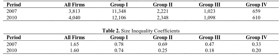
Table 1 provides some information about the average firm size, measured by their sales, in all firms as well as in each group over two selected years, 2007 and 2010. It shows a slight increase in the average size of firm from 2007 to 2010 despite the 2008 worldwide financial crisis. It also points out that the average firm size of Group I is significantly larger than that of the sample as a whole, while that of the other three groups falls below the sample average in both years. Table 2 presents a summary measure of firm size inequality, as indicated by the coefficient of variation. It shows that the first group has the highest concentration. However, the firm size inequality coefficients followed a decreasing trend, i.e., less concentration in 2010 relative to 2007, especially for the three smaller firm size groups.
Table 1. Average Size of Firms (In Million Dollars)
Period All Firms Group I Group II Group III Group IV
2007 3,813 11,348 2,221 1,023 659
2010 4,040 12,106 2,348 1,098 610
Table 2. Size Inequality Coefficients
Period All Firms Group I Group II Group III Group IV
2007 1.65 0.78 0.69 0.47 0.33
2010 1.60 0.74 0.25 0.18 0.20
Table 3 gives average growth rates for each group as well as all firms over the two sub-periods under study. It shows that the three smaller groups enjoyed growth rates in the range of 15-16%, outperforming the largest firm size group during 2006-2007. However, all groups faced with slower growth rates over the 2009-2010 period. This could be an indicator of the slow recovery after the economic crisis of 2008 and the recession of 2009. Nevertheless, Group III performed better than the other groups and still enjoyed a double digit growth rate.
Table 3. Average Growth Rates of Firms (%)
Period All Firms Group I Group II Group III Group IV
2006-2007 14.30 (0.41)
11.12 (0.15)
15.81 (0.44)
15.10 (0.27)
15.02 (0.61)
2009-2010 8.91
(0.22)
6.37 (0.18)
9.66 (0.15)
13.99 (0.33)
Table 4 provides information about the average profitability, measured by profits/sales ratios, for each group as well as all firms over the two selected years, 2007 and 2010. It shows no significant change in the overall average profitability in 2010 compared with that of 2007. However, while profitability slightly increased in the case of Group II, it jumped significantly for Group III but decreased in the cases of Group I and Group IV.
Table 4. Average Profitability of Firms (%)
Period All Firms Group I Group II Group III Group IV
2007 10.8 14.3 15.0 10.5 7.1
2010 10.4 13.4 15.1 17.6 5.8
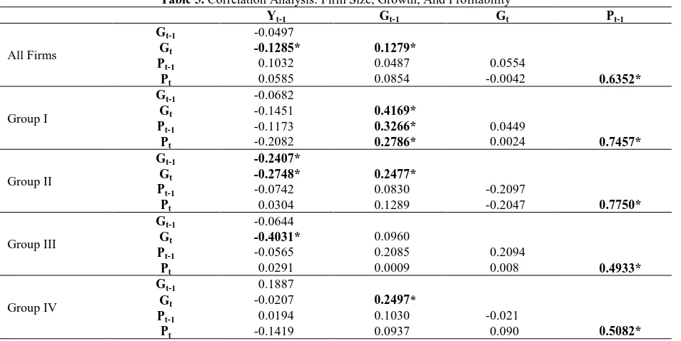
Table 5 reports the period-wise bivariate correlation coefficients between firm size (Y), growth (G), and profitability (P) for all firms pooled together as well as for each of the four groups of firms. Note that subscripts t-l and t refer to the beginning-of-the-period and the end-of-the-period values of the variable, respectively. The correlations
between Gt and Yt-1 are negative, indicating the disadvantage of size. However, these coefficients are not statistically
significant in the cases of Group I and Group IV. The reported significant correlations between Pt and Pt-1 imply
persistence of profits in all cases. According to Mueller (1977, 1986), firms use their current profits to protect future profits, employing various means such as product differentiation and ownership of scarce human and natural resources. This endogenous theory of the persistence of profit is also consistent with theories and empirical studies
relating persistently high profit rates to market structural variables. The correlation results between Gt and Gt-1 also
point to autocorrelated or persistent growth in all cases except for Group III. The persistence of growth may arise due to special talents or circumstantial advantages available to some growing firms who continue to enjoy a higher-than-average growth rate. See, Singh and Whittington (1975) and Chesher (1979). Note that the persistence of growth is in violation of Gibrat’s law that growth of firms is random, and thus, is independent of systematic influences such as past growth rates.
Table 5. Correlation Analysis: Firm Size, Growth, And Profitability
Yt-1 Gt-1 Gt Pt-1
All Firms
Gt-1 -0.0497
Gt -0.1285* 0.1279*
Pt-1 0.1032 0.0487 0.0554
Pt 0.0585 0.0854 -0.0042 0.6352*
Group I
Gt-1 -0.0682
Gt -0.1451 0.4169*
Pt-1 -0.1173 0.3266* 0.0449
Pt -0.2082 0.2786* 0.0024 0.7457*
Group II
Gt-1 -0.2407*
Gt -0.2748* 0.2477*
Pt-1 -0.0742 0.0830 -0.2097
Pt 0.0304 0.1289 -0.2047 0.7750*
Group III
Gt-1 -0.0644
Gt -0.4031* 0.0960
Pt-1 -0.0565 0.2085 0.2094
Pt 0.0291 0.0009 0.008 0.4933*
Group IV
Gt-1 0.1887
Gt -0.0207 0.2497*
Pt-1 0.0194 0.1030 -0.021
Pt -0.1419 0.0937 0.090 0.5082*
THE MODEL, THE ESTIMATION STRATEGY, AND EMPIRICAL RESULTS
Consider first the following log linear regression model for testing Gibrat’s law of proportionate effect for a set of firms surviving over a period of time:
lnYijt = 1 + 2 lnYijt-l + uijt (1)
where Yij represents the size of the i th
firm in the jth group. As noted before subscripts t-l and t refer to the
beginning-of-the-period and the end-of-the-period values of Y, respectively. 1 and 2 are parameters, and u’s are the
stochastic disturbances.
In this model, the Gibrat’s law of proportionate effect holds if 2 = 1, i.e., firm growth is independent of size.
If 2 < 1, smaller firms are expected to grow faster, and if 2 > 1 then the opposite would be true. However, the
estimation of this model by ordinary least squares (OLS) would be open to serious question if, as is likely, there is serial correlation in the random term uijt; see for example Chesher (1979). Define the growth rate of the ith firm in the jth group
at time t as Gijt=(Yijt-Yijt-l)/Yijt-l and using Taylor expansion then combining with equation (1) it approximately holds that
Gijt = α1 + (2 - 1) lnYijt-1 + uijt (2)
On the basis of the assumption that the u's are generated by the first- order autoregressive scheme,
Gijt = α1(l - ρ) + (α2 - 1) (l - ρ) lnYijt-1 + α2ρ Gijt-1 + vijt (3)
where ρ is the coefficient of autocorrelation and v’s are serially uncorrelated. Now let β1 = α1 (l- ρ), β2 = (α2 - l)(l- ρ),
and β3 = α2ρ.This yields
Gijt = β1 + β2lnYijt-1 + β3Gijt-1 + vijt (4)
The model expressed in equation (4) can now be used to conduct direct tests concerning the relationship between firm growth rate and its initial size as well the persistence of growth. However, if the ordinary least squares estimation method is used, any test about the parameters would be open to serious question if, as is likely, there is heteroscedasticity in the disturbance term; see for example Prais (1976), Chesher (1979), and Jovanovic (1982). In the above model, managerial/organizational differences among these firms are assumed away by virtue of the assumption that all coefficients are the same across these firms. This is a questionable assumption a priori; at least one that should be treated as a testable proposition. Following AmirKhalkhali and Dar (1993), this paper deals with these issues by adopting the more general varying coefficients model, which treats the fixed-coefficients assumption as a testable proposition. In addition, the varying coefficients model can be seen as a refinement of the stochastic law relating growth to its main determinants [see Pratt and Schlaifer (1988)]. Accordingly, the following model is estimated in this study:
Gijt = β1j + β2j lnYijt-l + β3jGijt-1 + ijt (5)
Note that (5) is a varying coefficients model, and that the new disturbance term is not the joint effect of excluded variables; instead, it is the joint effect of the remainder of the excluded variables after the effect of included variable has been factored out. The varying coefficients model represented by (5) is more general than those employed in previous studies because not only it describes more correctly the law relating the dependent variable to its determinant, but it also permits the impact to be group-specific.
Table 6. Pooled RGLS Results: Gijt = 1j + 2j ln Yijt-1 + 3j Gijt-1 + εijt
FIRMS β1 β2 β3
Pooled 1.4564
(1.0985)
-0.0981 (0.0782)
0.0965 (0.1403) G-Statistic = 32.42*
*Figures in brackets are standard errors.
The reported results in Table 6 show that the null hypothesis of no relationship between size and growth embodied in the law, i.e., 2 =0, as well as the persistence of growth, i.e., 3 =0 cannot be rejected for pooled data. In
other words, these pooled results support Gibrat’s law. It also reports a statistically significant Statistic. The G-statistic, which follows 2distribution, rejects the null hypothesis of fixed coefficients and supports the application of varying coefficients approach in this case. In other words, the RGLS pooled results in Table 6 do not refute Gibrat’s law but point to differences among the four groups. In light of this, the Swamy and Mehta (1975) RGLS method is used to estimate the varying coefficients model for each group over the two periods of 2006-2007 and 2009-2010. For more details of the RGLS estimation method and G-statistic, see AmirKhalkhali and Dar (1993), and Swamy and Tavlas (1995, 2002).
Table 7. Group-Wise RGLS Results: Gijt = 1j + 2j Ln Yijt-1 + 3j Gijt-1 + εijt
FIRMS β1j β2j β3j
Group I 0.5057* -0.0302 0.3748*
Group II 1.1130* -0.0713* 0.0783
Group III 2.9054* -0.2723* -0.1374
Group IV 0.3017 -0.0187 0.0701*
*Denotes significantly different from zero at the 0.05 level or less.
Table 7 reports the RGLS group-wise results. These results appear to shed more light on the somewhat aggregate results of Table 6. For more details of the RGLS estimation method and G-statistic, see AmirKhalkhali and Dar (1993), and Swamy and Tavlas (1995, 2002).
The results presented in Table 7 show that Gibrat’s law does not hold in the cases of all four groups because of the significance of the impact of size (Group II and Group III) or that of the persistence of growth (Group I and Group IV). The negative results for 2j imply faster growth for smaller firms than larger ones in all cases. Nevertheless, Table 7
shows that the degree of disadvantage of size on growth appears to be somewhat different for each group. It reports the largest negative impact of size on firm growth for Group III and the smallest impact for Group IV. However, it also shows a very small and insignificant impact of size on growth as well as a very large and significance persistence of growth for Group I.
SUMMARY AND CONCLUDING REMARKS
the case of the routinized regime, while the latter case is termed the entrepreneurial regime. However, it should be noted that the growth of firms could be explained by systematic forces if one could identify special resources and opportunities generating this growth. Valuable insights may be gained by such micro-studies.
AUTHOR INFORMATION
Dr. Atul Dar is a full professor in the Department of Economics, Sobey School of Business, at Saint Mary’s University. He is also the Chairperson of the Department, and Acting Academic Director of the Master of Applied Economics program. His research has been published in refereed journals such as: Applied Economics, Canadian Journal of Economics, Economic Modelling, Economic Notes, Empirical Economics, IMF Staff Papers, Journal of Development Studies, Journal of Risk and Insurance, Journal of Policy Modelling, Review of Applied Economics, and Southern Economic Journal.
Dr. AmirKhalkhali has been at Saint Mary's University since 1984, and is a full professor in the Department of Economics since 1996. His publications include book chapters and articles in journals such as Canadian Journal of Economics, Canadian Public Administration, Canadian Public Policy, Canadian Tax Journal, Applied Economics, Development Policy Review, Eastern Economic Journal, Economic Modelling, Economic Notes, Empirical Economics, IMF Staff Papers, Journal of Policy Modelling, Southern Economic Journal, Communications in Statistics, Sankhya, Journal of Statistical Computation and Simulation, and The Statistician.
REFERENCES
Acs, Z.J. and Audretsch, D.B. (1988), “Innovation in Large and Small Firms: An Empirical Analysis”, American Economic Review, 78, 678-690.
AmirKhalkhali, S. and Dar, A. (1993). “Testing for Capital Mobility: A Random Coefficients Approach”, Empirical Economics, 18, 523-541.
AmirKhalkhali, S. and Mukhopadhyay, A. K. (1993). “The influence of Size and RD on the Growth of Firms in the U.S.”, Eastern Economic Journal, 19(2), Spring, 223-233.
Audretsch, D.B. (1995), “Innovation, Growth and Survival”, International Journal of Industrial Organization, 13, 441-457.
Buckley, P.J., Dunning, J.H. and Pearce, R.D. (1984), “An Analysis of the Growth and Profitability of the World's Largest Firms. 1972 to 1977", Kyklos. 37(1), 3-26.
Chesher, A. (1979). “Testing the Law of Proportionate Effect”, Journal of Industrial Economics, June, 403-11. Coad, Alex. (2007). Firm Growth: A Survey, Manuscript, Max Plank Institute of Economics.
Cowling, M. (2004). “The Growth - Profit Nexus”, Small Business Economics, 22, 1-9.
Droucopoulos, V. (1982), "International Big Business, 1957-77: A Sequel on the Relationship between Size and Growth", Journal of Economic Studies, 9(3), 3-19.
Droucopoulos, V. (1983), "International Big Business Revisited: On the Size and Growth of the World's Largest Firms". Managerial Decision Economics. Dec., 4(4), 244-52.
Evans, D. E. (1987), "The Relationship between Firm Growth, Size, and Age: Estimates for 100 Manufacturing Industries", Journal of Industrial Economics, June, 567-81.
Gibart, R. (1931), "Les Inégalités économiques", Paris, France.
Gort, M. and Klepper, S. (1982), “Time Paths in the Diffusion of Product Innovations”, Economic Journal, 92, 630-653.
Hall B.H. (1987), "The relationship between firm size and firm growth in the US manufacturing sector". The Journal of Industrial Economics. June, 35(4), 583-606.
Hart, P. E. and Oulton, N. (1996), “Growth and Size of Firms”, Economic Journal, September, 1242-1252. Ijiri, Y. and Simon, H. A., (1974), "Interpretations of Departures from the Pareto Curve Firm-Size Distributions",
Journal of Political Economy, March/ April, 315-31.
Ijiri, Y. and Simon, H. A., (1977), Skew Distributions and the Sizes of Business Firms, North Holland Publishing, Boston.
Kamien, M.I. and Schwartz, N.L. (1982), Market Structure and Innovation, Cambridge University Press.
Kumar, M.S. (1985), "Growth, Acquisition Activity and Firm Size: Evidence from the United Kingdom", Journal of Industrial Economics. March, 33(3), 327-38.
Marris, R. (1964), The Economic Theory of Managerial Capitalism, Macmillan: London, 1964.
Mukhopadhyay A.K. and Amirkhalkhali, S. (2004). “Technological opportunity and the growth process of firms”, Journal of Academy of Business and Economics, 3(1), 111-116.
Mukhopadhyay, A. K. (1985), "Technological Progress and Change in Market Concentration in the U.S., 1963-1977", Southern Economic Journal, vol. 52, no. 1, July, 141-49.
Mueller, D.C. (1977), “The Persistence of Profits Above the Norm”, Economica, 44, 369-380. Mueller, D.C. (1986), Profits in the Long-run, Cambridge University Press.
Nassar, I.A., Almsafir, M.H., and AlMarouq, M.H. (2013), “The Validity of Gibrat’s Law in Developing Countries”, Journal of Advanced Social Research, June, 154-163.
Nelson, R. R. and Winter, S. G. (1978), "Forces Generating and Limiting Concentration under Schumpeterian Competition," Bell Journal of Economics, Autumn, 524-48.
Nelson, R. R. and Winter, S. G. (1982a), "The Schumpeterian Tradeoff Revisited", American Economic Review, vol. 72, no. 1, March, 114-132.
Nelson, R. R. and Winter, S. G. (1982b), An Evolutionary Theory of Economic Change, Cambridge, Mass: Harvard University Press.
Penrose, E.T. (1959), The theory of the growth of the firm, Blackwell, Oxford.
Prais, S. J., (1976), The Evolution of Giant Firms in the UK” Cambridge: Cambridge University Press.
Pratt J. W. and Schlaifer, R. (1988) “On the Interpretation and Observation of Laws”, Journal of Econometrics 39, 23-52.
Schumpeter, J.A. (1950), Capitalism, Socialism and Democracy, Third Edition, George Allen & Unwin, London. Simon, H. A. (1955), "On a Class of Skew Distribution Functions", Biometrica, 42, 425-40.
Singh, A. and Whittington, G. (1975), "The Size and Growth of Firms", Review of Economic Studies. Jan., 42, 15-26. Sutton, John (1997), “Gibrat’s Legacy”, Journal of Economic Literature”(35,1), March, 40-59.
Swamy, P.A.V.B., (1970), “Efficient Inference in a Random Coefficients Regression Model”, Econometrica 38, 3ll-23.
Swamy, P.A.V.B. and Mehta, J.S., (1975), “Bayesian and Non-Bayesian Analysis of Switching Regressions and of Random Coefficient Regression Models”. Journal of the American Statistical Association, 70, 593-602. Swamy, P.A.V.B. and Tavlas, G.S. (2002), “Random Coefficient Models: Theory and Applications”, Journal of
Economic Surveys, 165-196.
Swamy, P.A.V.B., and Tavlas, G.S. (2002), Random Coefficient Models. In Baltagi, B.H. (Ed.) Companion to Theoretical Econometrics, Basil Blackwell, 2002, 410-428.