www.nat-hazards-earth-syst-sci.net/10/1431/2010/ doi:10.5194/nhess-10-1431-2010
© Author(s) 2010. CC Attribution 3.0 License.
and Earth
System Sciences
Mesopause temperature perturbations caused by infrasonic waves
as a potential indicator for the detection of tsunamis and
other geo-hazards
M. Bittner, K. H¨oppner, C. Pilger, and C. Schmidt
German Remote Sensing Data Center (DFD), German Aerospace Center (DLR), Oberpfaffenhofen, Germany Received: 31 March 2010 – Revised: 31 May 2010 – Accepted: 6 June 2010 – Published: 2 July 2010
Abstract. Many geo-hazards such as earthquakes, tsunamis, volcanic eruptions, severe weather, etc., produce acoustic waves with sub-audible frequency, so called infrasound. This sound propagates from the surface to the middle and up-per atmosphere causing pressure and temup-perature up- perturba-tions. Temperature fluctuations connected with the above mentioned events usually are very weak at the surface, but the amplitude increases with height because of the exponential decrease of atmospheric pressure with increasing altitude. At the mesopause region (80–100 km height) signal amplitudes are about two to three orders of magnitude larger than on the ground.
The GRIPS (GRound-based Infrared P-branch Spectrome-ter) measurement system operated by the German Remote Sensing Data Center of the German Aerospace Center (DLR-DFD) derives temperatures of the mesopause region by ob-serving hydroxyl (OH) airglow emissions in the near infrared atmospheric emission spectrum originating from a thin layer at approximately 87 km height.
The GRIPS instrument is in principle suited for the de-tection of infrasonic signals generated by e.g. tsunamis and other geo-hazards. This is due to the fact that the infra-sound caused by such events should induce observable short-period fluctuations in the OH airglow temperatures. First re-sults obtained during a field campaign performed at the Envi-ronmental Research Station “Schneefernerhaus”, Zugspitze (47.4◦N, 11.0◦E) from October to December 2008 are pre-sented regarding potential sources of meteorological and oro-graphical origin.
Correspondence to: M. Bittner
An adequate distinction of the overlapping infrasonic sig-natures caused by different infrasound sources in the OH temperature record is needed for the ascription to the proper source. The approach presented here could form a contribu-tion to a hazard monitoring and early warning system.
1 Introduction
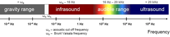
16 Hz, which is in the sub-audible range. Infrasound is on the other hand limited by the acoustic cut-off frequency at about 0.003 Hz, which separates sound from gravity waves. This frequency range corresponds to signal periods of 0.05 s up to 5 min (see Fig. 1).
Sound waves are longitudinal waves because wave dis-turbances travel parallel to the direction of wave propaga-tion. They occur in the atmosphere when a periodic vibra-tion causes alternating adiabatic compression and expansion of air. In each wave induced compression cycle of the gas there will be a temperature increaseT0(see Liszka, 1977):
T0=u
c(γ−1)T (1)
wherecis the sound velocity,uthe particle velocity,γ the specific heat ratio andT the ambient temperature. Assum-ing an infrasonic source signal of a certain initial pressure amplitude, one can calculate the expected particle velocities and resulting temperature perturbations occurring in a speci-fied layer of the atmosphere as e.g. in the mesopause airglow layer at∼87 km height (see Sect. 2.2). The effects of infra-sound on the middle and upper atmosphere in terms of tem-perature fluctuations have been quantified by e.g. Schubert et al. (2005), Krasnov et al. (2007) or Pilger and Bittner (2009). Neither pressure nor temperature fluctuations in the at-mosphere can be easily measured above the stratosphere. Aircrafts and balloons do not reach such altitudes. Rocket measurements are sparse and expensive and satellite based measurements do not usually provide the spatial resolution needed for infrasound detection. However, a number of tech-niques have been developed during the past decades that al-low indirect detection of the temperature in higher altitudes. One of them is the remote sensing of the airglow in the mesopause region (80–100 km altitude). The airglow is elec-tromagnetic radiation emitted in the upper mesosphere in the visible and near infrared due to atomic and molecular ex-citations at these heights. One prominent airglow source is a rather narrow layer of excited hydroxyl (OH) molecules from about 83–90 km height peaking around about 87 km (e.g. Baker and Stair, 1988). The excitation is caused by the exothermic reaction of ozone and atomic hydrogen (Bates and Nicolet, 1950; Meinel, 1950a).
measurement of the hydroxyl airglow spectra is a well estab-lished technique which is being routinely performed around the globe at many measurement stations (see e.g. Beig et al., 2003, and references therein) of which many have re-cently formed the Network for the Detection of Mesopause Change (NDMC; http://wdc.dlr.de/ndmc). These airglow de-rived temperatures have been used for example for studying planetary waves with periods from days to weeks (e.g. Sivjee et al., 1994; Espy et al., 1997; Takahashi et al., 2002; Bu-riti et al., 2005; H¨oppner and Bittner, 2007; L´opez-Gonz´alez et al., 2009) as well as for investigating atmospheric grav-ity waves with periods of several hours down to about 8 min (e.g. Gavrilov et al., 2002; Reisin and Scheer, 2004).
Time series of OH temperatures occasionally show signa-tures of periods even below 5 min if the temporal resolution of the used instrument is sufficiently high. Possible sources of such small-scale signatures are infrasonic signals.
The German Remote Sensing Data Center (DLR-DFD) operates the GRIPS (GRound-based Infrared P-branch Spectrometer) instruments for the measurement of hydroxyl airglow intensities with high temporal resolution (Bittner et al., 2002). First tests for detecting specific infrasound signals were performed during a measurement campaign at the Environmental Research Station Schneefernerhaus (UFS, 47.4◦N, 11.0◦E) at the Mountain Zugspitze in southern Ger-many during October–December 2008. The detection and identification of signals in the infrasound low frequency regime, most likely generated by meteorological activities and the Alpine orography, was achieved using a new detector technology which delivers the required high temporal resolu-tion measurements.
Fig. 2. Concept of infrasound generation and propagation, its impact on the mesospheric hydroxyl layer and the resulting radiation measured
by the ground based infrared spectrometer GRIPS (see text for details).
law assumptions. These perturbations modulate the OH tem-peratures on their travel through the airglow layer in the mesopause region. Using the measurement technique of in-frared spectroscopy with sufficient high temporal resolution in conjunction with a versatile signal classification algorithm, it should be possible to detect and identify the signals asso-ciated with geo-hazards such as a tsunami. If this can be re-liably demonstrated then the measurement system could be deployed for the rapid detection of such hazards.
The study presented is part of the GITEWS (German-Indonesian Tsunami Early Warning System) project (Rudloff et al., 2009).
The paper is organized as follows. The modeling of in-frasound propagation, the quantification of infrasonic ef-fects and first comments on signal parameters is presented in Sect. 2. The measurement principle as well as a descrip-tion of the instrumentadescrip-tion is given in Sect. 3. In Sect. 4 preliminary results of infrasound induced temperature fluc-tuations recorded during a few weeks measurement period are presented.
2 Modeling approach
2.1 Infrasound propagation modeling
The propagation of infrasound from a surface source to the mesopause region and higher can be modeled with e.g. ray-tracing methods (see Jones et al., 1986; Drob et al., 2003; Pilger and Bittner, 2009). The ray-path calculations are performed using the Hamilton equations of motion and are solved numerically by use of the HARPA program (Hamilto-nian Ray-Tracing Program for Acoustic Waves in the Atmo-sphere; Jones et al., 1986). HARPA is a commonly used and well established numerical code for 3-D infrasonic
ray-tracing. Atmospheric background conditions such as the pressure-, temperature-, and wind-profiles are an inte-gral part for the propagation calculations for infrasound. The HARPA code was modified by including climatologies for atmospheric background conditions (see below). The modi-fied version is denoted as HARPA/DLR (Pilger and Bittner, 2009).
The climatology NRL-MSISE-00 (Naval Research Laboratories-Mass Spectrometer and Incoherent Scatter Radar; Picone et al., 2002) is used for the representation of atmospheric temperatures. For the modelling of wind fields the HWM-93 (Horizontal Wind Model; Hedin et al., 1996) was chosen. A further aspect of propagation modelling is the influence of signal attenuation. The influence of geometric spreading (weakening of a signal with range due to expansion) and atmospheric attenuation (damping due to thermal and molecular processes) is also considered in the improved HARPA/DLR program code.
Fig. 3. A typical infrasound propagation pattern of a surface point
source including acoustic loss due to atmospheric attenuation and geometric spreading, modelled with HARPA/DLR. The signal loss is coloured and given in the relative unit of decibel.
Fig. 4. MSISE-00 output for the monthly mean temperature profile
at Munich, Germany (48.1◦N, 11.6◦E). The strong positive tem-perature gradients in the stratosphere and lower thermosphere lead to acoustic ray reflections and surface returns (so-called “ducts”). There are also strong seasonal influences like the cold (warm) mesopause in summer (winter).
The so-called “ducting” of acoustics rays and their returns to the surface are predominantly caused by strong tempera-ture gradients in the atmosphere. These gradients mainly ap-pear in the stratosphere (“stratospheric duct”) and the lower thermosphere (“thermospheric duct”), where the temperature strongly increases. The influences of horizontal wind on the propagation were found to be of secondary importance, but not negligible in the context of background modelling.
Figures 4 and 5 show model outputs of MSISE-00 of monthly means of temperature and zonal wind fields calcu-lated, for example, for Munich, Germany (48.1◦N, 11.6◦E). Seasonal structures in the temperature and the zonal wind have a significant effect on the wave propagation in the at-mosphere. The semi-annual wind reversal in the stratosphere is well represented by the HWM-93 model. It has been men-tioned above that realistic temperature and wind data are
re-Fig. 5. HWM-93 output for monthly mean zonal wind profiles at
Munich, Germany (48.1◦N, 11.6◦E). The changing direction of the stratospheric wind jet from winter to summer leads especially to horizontal variations in the propagation pattern of infrasound.
quired to allow for precise infrasound propagation predic-tion. Smaller scale perturbations in temperature and wind of a few degree Kelvin or m/s, respectively, can seriously alter the sound propagation. Therefore, the climatologies also take into account daily and hourly variations (not shown here). The exact date and daytime is a significant input to the HARPA/DLR-modelling.
2.2 Quantification of infrasound temperature fluctuations
A subsequent aspect of propagation modelling is the calcula-tion of singular temperature effects due to the passage of an infrasonic signal through the atmosphere. The temperature perturbationT0(see Eq. 1) depends primarily on the particle velocityu. Various processes increase and decrease this par-ticle velocity such as geometric spreading loss, atmospheric attenuation loss and amplification with decreasing air den-sity. They will be further discussed below.
the inverse surface increase, so it is proportional to 1/r. The sound intensityI is also proportional to the square of particle velocityuand therefore:
I∝u2∝1
r ⇒u∝
1
√
r (2)
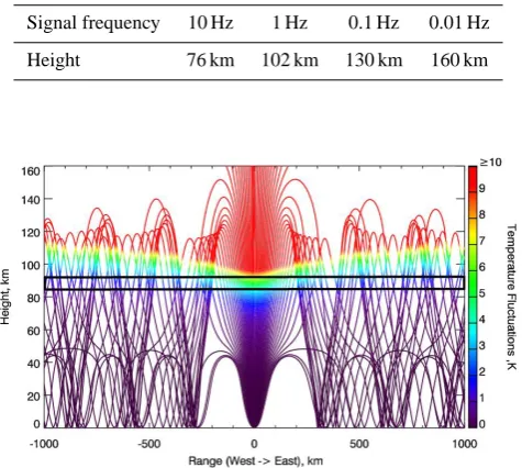
Atmospheric attenuation loss (see e.g. Evans et al., 1972) characterizes the weakening of a signal due to damping pro-cesses. These processes are subdivided into classical losses (i.e. losses due to viscosity and thermal conductivity of air), diffusion losses and relaxation losses. The classical pro-cesses are the most significant ones for middle and upper at-mospheric attenuation. Diffusion only contributes with 0.3% to the total attenuation of a signal and relaxation dominates only in the lower to middle atmosphere, where the overall attenuation is still very weak. The attenuation is frequency-dependent and increases with height. Typical heights, where the loss due to attenuation becomes stronger than the ampli-fication due to decreasing air density (described below) are given in Table 1. The attenuation coefficients for the different attenuation processes can be quantified using HARPA/DLR. The total absorptionAin decibels can be calculated over a specified distance of propagation; the loss of sound intensity
Iand particle velocityudue to attenuation can be expressed by (Pilger and Bittner, 2009):
I∝u2∝10−A/10⇒u∝10−A/20 (3) Amplification with decreasing air density is a process that increases signal amplitude with height. The exponential de-crease of air density with height can be represented by the following scale height relation:
ρ=ρ0e−z/H (4)
whereρis the air density,ρ0the air density at surface level (∼1.225 kg/m3),zthe height and H the atmospheric scale height (∼6.8 km as an approximation for all altitudes from ground to lower thermosphere). The squared particle veloc-ityu2of a sound signal has to increase in the same way as the air densityρdecreases if energy conservation (and therewith constant intensityI) is assumed:
I=u2ρ c⇒u∝√1
ρ (5)
Following Eqs. (2), (3), and (5) the particle velocity u is proportional to the inverse square root of distance and pres-sure and the inverse scaled attenuation over 20. Therefore, if both, the distance and the attenuation increases, the parti-cle velocity decreases. If the pressure decreases, the partiparti-cle velocity increases. Due to the fact that the background air pressure decreases exponentially with height (Eq. 4), the in-crease of the square of particle velocity is also exponential and it exceeds the decrease due to the other effects until at-tenuation becomes dominant. Following Eq. (1), the temper-ature fluctuationT0increases in the same way as the particle velocityu.
Table 1. Frequency-dependent height, where the processes of
atmo-spheric attenuation start to dominate compared to the amplification by decreasing of air density.
Signal frequency 10 Hz 1 Hz 0.1 Hz 0.01 Hz
Height 76 km 102 km 130 km 160 km
Fig. 6. Temperature fluctuation for a signal of 0.01 Hz frequency
and 100 Pa pressure amplitude (at 1 km initial distance from the source) using cylindrical spreading implemented in HARPA/DLR. The OH layer between 83 and 91 km is marked by a rectangle.
Figure 6 shows an example of a temperature fluctuation development with height and range. It has been calculated using HARPA/DLR (for more details see Pilger and Bitt-ner, 2009). With increasing height the decreasing air den-sity leads to an exponential increase of the fluctuation. The temperature fluctuations in the OH layer (ca. 87±4 km) are largest directly above a source. Shown is an example case us-ing strong sound amplitude of 100 Pa (at 1 km initial distance from the source) and weak attenuation for a low frequency of 0.01 Hz. The expected temperature fluctuation amounts
∼5 K in the OH layer for this signal. 2.3 Infrasound signal identification
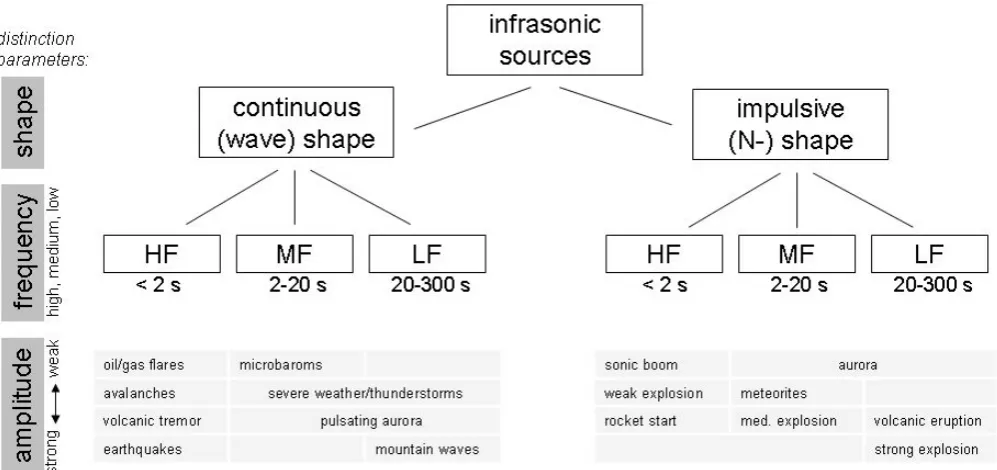
A pattern recognition algorithm is needed in order to reli-ably identify and classify infrasound signals in the OH tem-perature fluctuations originating from different sources. The source characteristics, which can be used to distinguish dif-ferent signals, are sound frequency, sound amplitude and sound waveform.
Fig. 7. Distinction scheme for infrasonic sources using the parameters of sound amplitude, frequency and waveform. See text for further
details.
frequencies can vary by one or two orders of magnitude. For example, explosion frequencies are yield-dependent: the stronger an explosion, the longer its period. Other prominent long-period (>20 s) signals are mountain-associated infra-sound waves, severe weather and volcanic eruptions, while short-period signals are e.g. due to avalanches, sonic booms and volcanic tremors (see Fig. 7).
A second discrimination parameter in this context is the pressure amplitude of a sound signal. Infrasonic signals vary from nearly undetectable milli-Pascal effects to shock-waves of some hundreds to thousands of Pascal. The most important parameter for amplitude calculations is the dis-tance from the source. This is due to the fact that the sound amplitude predominantly decreases with distance due to geometric spreading loss. This loss is estimated using the above-mentioned ray tracing method (see Sect. 2.1) for the determination of the distance between the signal and its source at a certain time and geometric spreading calculations (see Sect. 2.2) for the quantification of amplitude reduction. As mentioned above, infrasonic signals with weak ampli-tudes are microbaroms, meteorites, sonic booms and severe weather activities, while stronger signals are due to volcanic, explosive or eruptive activities (see Fig. 7).
A third parameter is the waveform of a sound signal. The discrimination of impulsive signals (with strong peaks or so-called “N-shapes”) and continuous signals (with wave-like or alternating characteristics) strongly depends on the in-strumental capabilities to detect those waveforms. In a first approach, sonic booms, explosions and eruptions are deter-mined to be impulsive while microbaroms, earthquakes and volcanic activity are continuous (see Fig. 7).
Figure 7 shows a distinction scheme for several of the most common infrasound sources by the parameters frequency, amplitude and waveform. It reflects the first steps to be per-formed in signal classification and discrimination. Two se-lected events regarding different infrasound sources are dis-cussed in Sect. 4. Further investigations concerning pattern recognition of infrasonic signals are beyond the scope of this paper.
3 Measurement technique and instrumentation
The hydroxyl (OH) airglow originates from a thin layer of about 8 km thickness at a peak altitude of about 87 km (e.g. Baker and Stair, 1988). The OH molecules are formed in an exothermic reaction of ozone with atomic hydrogen (Bates and Nicolet, 1950):
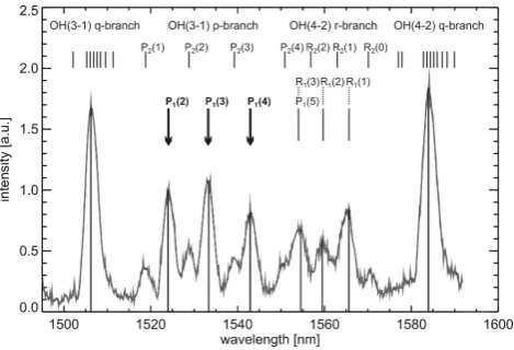
Fig. 8. OH nightglow emissions between 1.5 µm and 1.6 µm
mea-sured with the advanced GRIPS 5 spectrometer. Rotational tem-peratures are derived from the three strongest lines of the OH(3-1) p-branch: P1(2), P1(3), P1(4).
The relationship between the intensity of the emission linesI and the corresponding rotational temperatureTrotis given by Meinel (1950b):
I(ν0,J0,i→ν00,J00,i)=Nν0·A(ν0,J0,i→ν00,J00,i)
·2 2J
0+1
Qν0,T rot
·exp −
Fν0,J0,i
kBTrot
(7) whereNν0 andQν0,T
rotdenote the population number and the
state sum of the initial vibrational stateν0.AandFν0,J0,i
de-note the Einstein coefficient of spontaneous emission and the term value of the rotational level with respect to the vibra-tional levelν0and the doublet branchi. J0 is the quantum number of angular momentum andkB the Boltzmann con-stant. The temperature retrieval is based on the transition co-efficients from Mies (1974) and the rotational energy values from Krassovsky (1962).
The GRIPS spectrometers have been deployed for the ob-servation of OH airglow for nearly 30 years (see e.g. Bitt-ner et al., 2002; H¨oppBitt-ner and BittBitt-ner, 2007). The first in-struments were designed and built during the early 1980s at the University of Wuppertal, Germany (51.3◦N, 7.2◦E). More than two decades of experience and data have been gathered with this instrument series making it a promi-nent instrument in the history of airglow spectroscopy. At the end of this development line, GRIPS 6 – installed at DLR-DFD in Oberpfaffenhofen, Germany (48.1◦N, 11.3◦E) in 2009 – and the identically equipped GRIPS 5 – lo-cated at the Environmental Research Station Schneeferner-haus at Mt. Zugspitze, Germany (47.4◦N, 11.0◦E) – repre-sent advanced scanning spectrometers for near infrared air-glow observations. Both instruments routinely and automat-ically measure the OH temperatures night by night (data are available from the World Data Center for Remote Sensing of the Atmosphere, WDC-RSAT, and can be accessed via http://wdc.dlr.de/ndmc).
Originally, the GRIPS system is used to monitor climate signals and observe long-term trends in the mesopause re-gion (e.g. Bittner et al., 2000; H¨oppner and Bittner, 2007), to better understand the impact of atmospheric dynamics on larger-scale circulation, to validate satellite-based measure-ments and to evaluate climate and atmospheric models. In addition, high temporal resolution data obtained with the new spectrometers GRIPS 5/6 reveal temperature oscillations with periods below the Brunt-V¨ais¨al¨a period.
Key features of these spectrometers are a thermoelectri-cally cooled 512 pixel InGaAs-array and a high aperture polychromator. This new spectrometer design offers a tem-poral resolution of 15 s, well within the infrasound regime (see Fig. 1). The overall dimension of the system is com-paratively small with only 600×500×400 mm3(see Fig. 9). The field of view of GRIPS 5/6 is 7.9◦×7.9◦. While the GRIPS 6 is looking into zenith direction, the GRIPS 5 in-strument is looking at a zenith angle of 45◦into southward direction, so its field of view is located over Northern Italy (see Fig. 12).
In order to gain reliable estimates of the uncertainty of the derived temperature values, the signal-to-noise ratio of each individual spectrum is derived by applying a low pass filter. The filtered spectrum gives a reliable estimate of the peak intensities, while the residuals are taken as their respec-tive uncertainties. This approach has proven to yield feasi-ble results in gaining the instrument’s precision. A conve-nient side effect of this approach is the fact that precision increases on longer time scales. As a consequence the uncer-tainty is typically of the order of 7.5 K for a 15 s exposure, while decreasing to values below 2 K at time scales of 1 min. Since the signal-to-noise ratio is a function of source inten-sity, atmospheric opacity and all possible influences caused by the instrument, the uncertainty of the derived tempera-tures strongly depends on the measurement conditions. Dur-ing the nights discussed in Sect. 4, temperature values range from 200 K to 240 K for the night of 2 to 3 November 2008 and from 180 K to 220 K for 5 to 6 November 2008, while the respective uncertainties of the 15 s values range between 7 K and 12 K for both nights (see Figs. 10, 11, 13, and 14). Thus the precision of the GRIPS instrument cannot explain the variability in our data and atmospheric waves are the likely explanation as is further confirmed by the results of the wavelet analysis.
4 Results and discussion
A field campaign SCARAMANGA1 at the Environmen-tal Research Station Schneefernerhaus in the German Alps (UFS, 47.4◦N, 11.0◦E) was conducted during October-December 2008. The GRIPS 5 spectrometer was deployed for this campaign to demonstrate the capability of this in-strumentation to detect low frequency infrasonic signals.
1Search for Characteristic Airglow Response to Autumnal
Fig. 9. Side view of the advanced GRIPS spectrometer.
Fig. 10. Nocturnal evolution of OH temperatures recorded
dur-ing the night from 5 to 6 November 2008 at the Environmental Research Station Schneefernerhaus (47.4◦N, 11.0◦E), Germany. 2466 spectra have been recorded by the GRIPS 5 spectrometer with a temporal resolution of 15 s.
During this campaign, 27 nighttime time series of up to 3000 OH spectra per night were recorded with a maximum temporal resolution of 15 s per spectrum. In order to check for shorter period fluctuations in the OH-temperature time series we performed a wavelet analysis. Wavelet analysis has proven to yield good results in atmospheric studies, es-pecially if spectral signatures are transient (e.g. W¨ust and Bittner, 2006; H¨oppner and Bittner, 2007; Bittner et al., 1998; Widdel et al., 1994). The wavelet analysis used in this study is based on the algorithm presented by Torrence and Compo (1998). Analyses using the Morlet wavelet function
Fig. 11. Wavelet spectrogram based on OH temperature time series
in Fig. 10 in the period range of 0.5 to 10 min. Colours indicate the wavelet power spectrum and white lines denote the 95% signif-icance level. Hatched areas are excluded due to edge effects of the wavelet analysis. A noticeable amount of wave activity is located around 20:00 UTC, 00:30 UTC and 04:00 UTC.
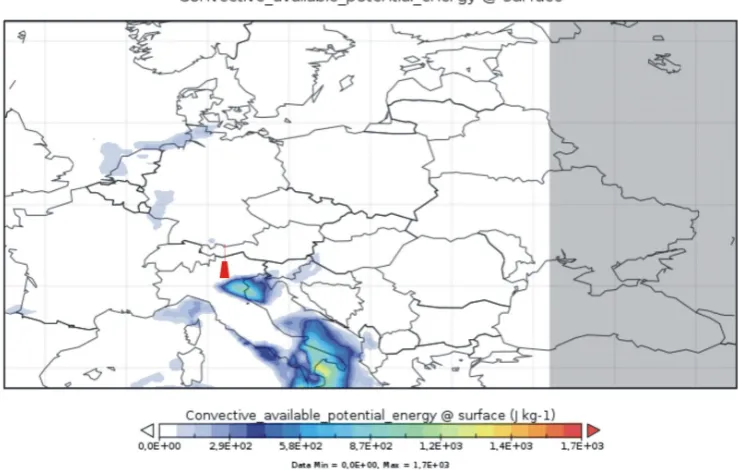
Fig. 12. ECMWF operational analysis of the convective available potential energy (CAPE) at surface level for the 6 November 2008,
00:00 UTC. Also shown is the location of GRIPS 5 at the Environmental Research Station Schneefernerhaus (47.4◦N, 11.0◦E) (red circle) and the field of view of the instrument (red trapeze). See text for further details.
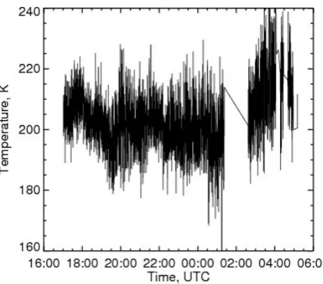
Fig. 13. The same as in Fig. 10, but for the night of 2 to 3 November
2008 from ca. 23:00 UTC to 05:30 UTC based on 1691 spectra.
Figures 10 to 15 show typical examples of nights with sig-nificant wave activity in the above mentioned period ranges indicating the impact of short period (infrasonic) signals on mesopause temperature time series.
Figure 10 shows the time series of OH(3-1) rotational temperatures obtained with the GRIPS 5 instrument during the night of 5 to 6 November 2008. A large data gap be-tween 01:15 UTC and 02:30 UTC is due to dense
cloudi-Fig. 14. The same as in cloudi-Fig. 11, but for the night of 2 to 3
Novem-ber 2008. A noticeable amount of wave activity is located around 04:00 UTC in a period range of 0.5 to 1.5 min (see also Fig. 15).
Fig. 15. Detail of Fig. 14 focusing on the measurement time
be-tween 03:39 UTC and 03:57 UTC and on periods below 5 min. An area of significant wave activity is located in the 1-min period range lasting about 10 min.
and 01:15 UTC and between 02:30 UTC and 05:00 UTC, re-spectively. Wave activity is observed in both, the short pe-riod gravity wave range with pepe-riods around 6 to 8 min (not discussed here) and the infrasonic period range with periods around 3 to 4 min. We speculate that the latter signatures may be attributed to a meteorological source, due to the fact that 3.5 min is a typical acoustic period of severe weather (see Georges, 1973; Chimonas and Peltier, 1974; Blanc, 1985). This is indeed in agreement with the fact that some thun-derstorm activity was recorded in Northern Italy through-out the whole night. Figure 12 shows the associated con-vective available potential energy (CAPE) for central Europe quantified by ECMWF operational analysis. A region of in-creased CAPE and therewith strong thunderstorm potential is centered at about 45◦N and 12◦E, which is located 300 km southward of the instrument and approximately 150 km from the center of the instrument’s field of view in the mesopause region. Infrasonic waves generated of the described thunder-storm source reach the field of view in a 150 km distance as seen in Fig. 6 and could therefore be detected by GRIPS 5 (see Fig. 11).
Figure 13 shows the temperature time series for the sec-ond half of the night from 2 to 3 November 2008, based on 1691 spectra in 15 s intervals. Especially the time frame near 04:00 UTC indicates short period wave activity between 30 and 90 s over at least 15 min of continuous duration (see Figs. 14 and 15). Orographical sources are a potential ex-planation for these signals. The so-called “mountain asso-ciated waves (MAWs)” are orographically generated infra-sonic waves in a typical period range of 20 to 60 s (e.g. Wil-son and OlWil-son, 2003). These lee waves occur when air is forced over a mountain ridge and is redirected vertically (e.g.
spectrometers GRIPS 5/6 for obtaining reliable high reso-lution spectra allowing the observation of OH temperature modulations caused by infrasonic waves traveling through the airglow layer.
The GRIPS system utilizes the so-called OH airglow phe-nomenon in 80–90 km altitude. Mesopause temperatures are currently routinely and automatically derived night-by-night from observations of hydroxyl (OH) emissions in the near infrared. The new IR-spectrometers GRIPS 5/6 measuring with a temporal resolution of 15 s allow the detection of short-period infrasound signals.
An infrasound propagation model was developed (HARPA/DLR) using the existing ray-tracing model HARPA and improving the propagation characteristics by including climatologies for atmospheric background condi-tions and taking into account the influence of attenuation on a signal. The development of a numerical infrasonic wave pattern recognition algorithm has been initiated.
To demonstrate and test the improved system’s perfor-mance and the developed modeling approach, a field cam-paign SCARAMANGA was conducted at the Environmental Research Station Schneefernerhaus (47.4◦N, 11.0◦E) from October to December 2008. It was shown that the GRIPS 5/6 instruments are able to measure signals in the period range of low frequency infrasound. The most likely sources of these detected signals are so-called mountain associated in-frasound waves generated by the orography of the Alps and meteorological sources such as thunderstorms.
It is concluded, that the measurement system GRIPS 5/6 is in principle suitable for the detection of geo-hazards pro-ducing infrasound. The deployment of GRIPS as an ad-ditional component in multi-hazard early warning systems could therefore increase the reliability of such systems.
In addition to the instrumental extension, the above-mentioned numerical infrasonic wave pattern recognition al-gorithm has to be further improved to better discriminate su-perimposed infrasound signatures in the airglow temperature records originating from different sources. Furthermore, the infrasound propagation modeling approach should be cou-pled with a numerical weather forecast model for a realistic consideration of the background atmospheric conditions in-stead of relying on climatologies as is currently done.
Finally, a comprehensive testing of the system is needed in the vicinity of different and well characterized infrasound sources.
Acknowledgements. The GITEWS project (German Indonesian Tsunami Early Warning System) is carried out through a large group of scientists and engineers from (GFZ) German Research Centre for Geosciences and its partners from the German Aerospace Center (DLR), the Alfred Wegener Institute for Polar and Marine Research (AWI), the GKSS Research Centre, the Konsortium Deutsche Meeresforschung (KDM), the Leibniz Institute for Marine Sciences (IFM GEOMAR), the United Nations Univer-sity (UNU), the Federal Institute for Geosciences and Natural Resources (BGR), the German Agency for Technical Coopera-tion (GTZ), as well as from Indonesian and other internaCoopera-tional partners. Funding is provided by the German Federal Ministry for Education and Research (BMBF), Grant 03TSU01. We also kindly acknowledge the support of the Environmental Research Station Schneefernerhaus, UFS, (http://www.schneefernerhaus.de) allowing us to perform the SCARAMANGA campaign. We also acknowledge ECMWF for providing the CAPE data. The authors thank the anonymous reviewers for their valuable comments.
Edited by: J. Lauterjung
Reviewed by: two anonymous referees
References
Baker, D. J. and Stair Jr., A. T.: Rocket measurements of the altitude distributions of the hydroxyl airglow, Phys. Scripta, 37, 611–622, 1988.
Bates, D. R. and Nicolet, M.: Atmospheric Hydrogen, Publications of the Astronomical Society of the Pacific, 62(365), 106–110, 1950.
Beig, G., Keckhut, P., Lowe, R. P., Roble, R. G., Mlynczak, M. G., Scheer, J., Fomichev, V. I., Offermann, D., French, W. J. R., Shepherd, M. G., Semenov, A. I., Remsberg, E. E., She, C. Y., L¨ubken, F. J., Bremer, J., Clemesha, B. R., Stegman, J., Sigernes, F., and Fadnavis, S.: Review of mesospheric temperature trends, Rev. Geophys., 41, 1015–1055, 2003.
Bittner, M., Offermann, D., Graef, H. H., and Donner, M.: Wavelet analysis of upper mesosphere temperature variations, Adv. Space Res., 21, 1445–1448, 1998.
Bittner, M., Offermann, D., and Graef, H. H.: Mesopause tempera-ture variability above a midlatitude station in Europe, J. Geophys. Res., 105, 2045–2058, 2000.
Bittner, M., Offermann, D., Graef, H. H., Donner, M., and Hamil-ton, K.: An 18-year time series of OH rotational temperatures
and middle atmosphere decadal variations, J. Atmos. Sol.-Terr. Phy., 64, 1147–1166, 2002.
Blanc, E.: Observations in the upper atmosphere of infrasonic waves from natural or artificial sources - A summary, Ann. Geo-phys., 3, 673–687, 1985,
http://www.ann-geophys.net/3/673/1985/.
Bowman, H. S. and Bedard, A. J.: Observations of Infrasound and Subsonic Disturbances Related to Severe Weather, Geophys. J. Int., 26(1–4), 215–242, 1971.
Buriti, R. A., Takahashi, H., Lima, L. M., and Medeiros, A. F.: Equatorial planetary waves in the mesosphere observed by air-glow periodic oscillations, Adv. Space Res., 35, 2031–2036, 2005.
Campus, P.: The IMS Infrasound Network and its Potential for De-tection of Events: Examples of a Variety of Signals recorded Around the World, Inframatics, 06, 13–22, 2004.
Chimonas, G. and Peltier, W. R.: On severe storm acoustic signals observed at ionospheric heights, J. Atmos. Terr. Phy., 36, 821– 828, 1974.
Dalgarno, A.: Vibrationally excited molecules in atmospheric reac-tions, Planet. Space Sci., 10, 19–28, 1963.
Drob, D. P., Picone, J. M., and Garc´es, M.: Global morphology of infrasound propagation, J. Geophys. Res., 108, 4680–4691, 2003.
Espy, P. J., Stegman, J., and Witt, G.: Interannual variations of the quasi-16-day oscillation in the polar summer mesospheric tem-perature, J. Geophys. Res., 102, 1983–1990, 1997.
Evans, L. B., Bass, H., and Sutherland, L.: Atmospheric Absorp-tion of Sound: Theoretical PredicAbsorp-tions, J. Acoust. Soc. Am., 51, 1565–1575, 1972.
Evers, L. G. and Haak, H. W.: Listening to sounds from an explod-ing meteor and oceanic waves, Geophys. Res. Lett., 28, 41–44, 2001.
Garc´es, M., Caron, P., and Hetzer, C.: Deep Infrasound radiated by the Sumatra Earthquake and Tsunami, EOS T. Am. Geophys. Un., 86(35), 317–320, doi:10.1029/2005EO350002, 2005. Gavrilov, N. M., Shiokawa, K., and Ogawa, T.: Seasonal variations
of medium-scale gravity wave parameters in the lower thermo-sphere obtained from spectral airglow temperature imager obser-vations at Shigaraki, Japan, J. Geophys. Res., 107, 4755–4764, 2002.
Georges, T. M.: Infrasound from Convective Storms: Examining the Evidence, Rev. Geophys., 11, 571–594, 1973.
Gossard, E. E. and Hooke, W. H.: Waves in the atmosphere: At-mospheric infrasound and gravity waves – Their generation and propagation, Atmospheric Science 2, Elsevier, New York, 1975. Hedin, A. E., Fleming, E. L., Manson, A. H., Schmidlin, F. J., Av-ery, S. K., Clark, R. R., Franke, S. J., Fraser, G. J., Tsuda, T., Vial, F., and Vincent, R. A.: Empirical wind model for the upper, middle and lower atmosphere, J. Atmos. Terr. Phys., 58, 1421– 1447, 1996.
H¨oppner, K. and Bittner, M.: Evidence for Solar signals in the mesopause temperature variability?, J. Atmos. Sol.-Terr. Phys., 69, 431–448, 2007.
Johnson, J. B., Lees, J. M., and Yepes, H.: Volcanic eruptions, lightning, and a waterfall: Differentiating the menagerie of infra-sound in the Ecuadorian jungle, Geophys. Res. Lett., 33, 6308– 6311, 2006.
2005 large Sumatra earthquakes and tsunami, Geophys. Res. Lett., 32, 19802–19806, 2005.
Liszka, L.: Infrasonic Waves – Interaction with the Atmosphere, in: Dynamical and Chemical Coupling Between the Neutral and Ionized Atmosphere, edited by: Grandal, B. and Holtet, J. A., NATO ASIC Proc., 35, 63–71, 1977.
L´opez-Gonz´alez, M. J., Rodr´ıguez, E., Garc´ıa-Comas, M., Costa, V., Shepherd, M. G., Shepherd, G. G., Aushev, V. M., and Sargoytchev, S.: Climatology of planetary wave type oscilla-tions with periods of 2-20 days derived from O2atmospheric and
OH(6-2) airglow observations at mid-latitude with SATI, Ann. Geophys., 27, 3645–3662, 2009,
http://www.ann-geophys.net/27/3645/2009/.
Lyra, G.: Theorie der station¨aren Leewellenstr¨omung in freier At-mosph¨are, ZAMM-Z. Angew. Math. Me., 23(1), 1–28, 1943. Meinel, A. B.: OH emission bands in the spectrum of the night sky.
Part IAstrophys. J., 111, 555–564, 1950a.
Meinel, A. B.: OH emission bands in the spectrum of the night sky. Part II, Astrophys. J., 112, 120–130, 1950b.
Mies, F. H.: Calculated vibrational transition probabilities of OH(X25), J. Mol. Spectrosc., 53, 150–188, 1974.
Mutschlecner, J. P. and Whitacker, R. W.: Infrasound from earth-quakes, J. Geophys. Res., 110, 1108–1118, 2005.
Pendleton, W. R., Espy, P. J., and Hammond, M. R.: Evidence for non-local-thermodynamic-equilibrium rotation in the OH night-glow, J. Geophys. Res., 98, 11567–11579, 1993.
Picone, J. M., Hedin, A. E., Drob, D. P., and Aikin, A. C.: NRLMSISE-00 empirical model of the atmosphere: Statistical comparisons and scientific issues, J. Geophys. Res., 107, 1468– 1483, 2002.
Pilger, C. and Bittner, M.: Infrasound from tropospheric sources: Impact on mesopause temperature?, J. Atmos. Sol.-Terr. Phy., 71, 816–822, 2009.
doi:10.5194/nhess-9-1381-2009, 2009.
Schubert, G., Hickey, M. P., and Walterscheid, R. L.: Physical pro-cesses in acoustic wave heating of the thermosphere, J. Geophys. Res., 110, 7106–7110, 2005.
Sivjee, G. G., Walterscheid, R. L., and McEwen, D. J.: Planetary wave disturbances in the Artic winter mesopause over Eureka (80◦N), Planet. Space Sci. 42, 973–986, 1994.
Sutherland, L. C. and Bass, H. E.: Atmospheric absorption in the atmosphere up to 160 km, J. Acoust. Soc. Am., 115, 1012–1032, 2004.
Takahashi, H., Buriti, R. A., Gobbi, D., and Batista, P. P.: Equato-rial planetary wave signatures observed in mesospheric airglow emissions, J. Atmos. Sol.-Terr. Phy., 64, 1263–1272, 2002. Torrence, C. and Compo, G. P.: A Practical Guide to Wavelet
Anal-ysis, B. Am. Meteorol. Soc., 79, 61–78, 1998.
Warfield, J. T. and Jacobson, M. J.: Invariance of geometric spread-ing loss with changes in ray parametrization, J. Acoust. Soc. Am., 50(1), 342–347, 1971.
Widdel, H., Bittner, M., and Hoppe, U.: Vertical velocities mea-sured at Biscarrosse and by EISCAT at Tromso during the DYANA campaign, J. Atmos. Terr. Phys., 56, 1779–1796, 1994. Wilson, C. R. and Olson, J. V.: Mountain Associated Waves at I53US and I55US in Alaska and Antarctica in the Frequency Passband from 0.015 to 0.10 Hz, Inframatics, 3, 6–10, 2003. W¨ust, S. and Bittner, M.: Non-linear resonant wave-wave