Nat. Hazards Earth Syst. Sci., 9, 1095–1109, 2009 www.nat-hazards-earth-syst-sci.net/9/1095/2009/ © Author(s) 2009. This work is distributed under the Creative Commons Attribution 3.0 License.
Natural Hazards
and Earth
System Sciences
Considerations on Swiss methodologies for rock fall hazard
mapping based on trajectory modelling
J. M. Abbruzzese, C. Sauthier, and V. Labiouse
Swiss Federal Institute of Technology of Lausanne (EPFL), Rock Mechanics Laboratory (LMR), Switzerland Received: 29 January 2009 – Revised: 26 May 2009 – Accepted: 7 June 2009 – Published: 9 July 2009
Abstract. Rock fall hazard assessment and hazard map-ping are essential for the risk management of vulnerable ar-eas. This paper analyses some issues concerning fragmen-tal rock fall hazard mapping methodologies. Two Swiss ap-proaches based on rock fall trajectory simulations results are presented. An application to a site in Switzerland emphasises the differences in the results, uncertainties related to hazard zoning procedures and the influence of some factors on the mapping process. In particular, the influence of a change in the temporal rock fall frequency, of the longer propagation along the slope of only a few computed blocks (defined in this sense as “extreme blocks”) and of the number of runs performed in trajectory modelling have been studied. Results are discussed with the purpose of achieving a more reliable and objective hazard analysis. The presented considerations are based on the Swiss Federal Guidelines, but many of them could be extended to other countries that evaluate rock fall hazard using an intensity-frequency diagram.
1 Introduction
Rock falls threaten several mountainous areas in many coun-tries in Europe, as well as worldwide. Methodologies for the analysis and zoning of the hazard due to rock falls have been developed to plan appropriate land use (Cascini et al., 2005) and to reduce the exposure to this kind of natural pro-cess. This also means reducing the potential losses in terms of both human lives and properties. Methods available to assess fragmental rock fall hazard on and beyond the base of talus slopes include geological, empirical and analytical methods (Hungr and Evans, 1988; Evans and Hungr, 1993).
Correspondence to: J. M. Abbruzzese ([email protected])
The geological approach is based on a detailed inspec-tion of deposits and rock fragments/boulders on the slope. The collected data may ascertain the past behaviour of the slope over a long time, which can then be used to predict the runout distance of future rock falls within a given return period (Evans and Hungr, 1993; Bunce et al., 1997). This method is however not relevant for all sites, e.g. when boul-ders may have a glacial or debris-flow origin.
The empirical evaluation of rock fall hazard results from several authors’ observations of the rock fall fragments and their distribution on talus slopes. Two methods are com-monly used for a preliminary estimation of the maximum rock fall reach: the rock fall Fahrb¨oschung (Onofri and Can-dian, 1979; Toppe, 1987) and the minimum shadow angle (Lied, 1977; Evans and Hungr, 1993). A 3-D generalisation of these approaches, called “cone method”, was suggested by Jaboyedoff and Labiouse (2003) to delineate the areas en-dangered by rock falls by using GIS data.
The analytical methods are computer-based models sim-ulating the trajectory of blocks which detach from a rock face. Under conditions of correct calibration, trajectory sim-ulations codes may be very helpful tools to determine areas at risk and to design adequate protection measures. Models are usually classified into two main categories: the rigorous and the lumped-mass methods (Hungr and Evans, 1988; Giani, 1992).
Hazard is expressed as the probability that a particular dangerous phenomenon (a fragmental rock fall, in this case), which may adversely affect human life, property or activity to the extent of causing disasters, occurs with a given inten-sity within a given period of time (Fell et al., 2005; ISDR, 2009). Intensity and frequency are thus key parameters for evaluating rock fall hazard and, for this purpose, some ap-proaches are based on the use of intensity-frequency ma-trix diagrams (Interreg IIc, 2001; Crosta and Agliardi, 2003; Corominas et al., 2003; Jaboyedoff et al., 2005). This paper is concerned with methodologies mapping fragmental rock
1096 J. M. Abbruzzese et al.: Considerations on Swiss methodologies for rock fall hazard mapping fall hazard according to intensity-frequency diagrams, and
some important difficulties and uncertainties which emerge when elaborating hazard maps from trajectory modelling re-sults.
The analysis of current available procedures underlines that one of the most difficult challenges in rock fall hazard as-sessment is to estimate the time recurrence of the events and the associated magnitude (Corominas and Moya, 2008). For this purpose, magnitude-frequency relationships have been proposed to define an association between the rock fall vol-ume and its probability of failure (Hungr et al., 1999; Dus-sauge at al., 2002; Hantz et al., 2003; Chau et al., 2003). The analysis of historical catalogues (Hantz et al., 2003; Co-pons, 2007) and dendrogeomorphology data (Corominas et al., 2005; Stoffel et al., 2005) are some of the methods which can help with giving a better insight into this issue. How-ever, depending on the study areas, this kind of data is not always available. Moreover, some mapping procedures are in fact not taking the temporal frequency of failure into ac-count (M.A.T.E./M.E.T.L., 1999; Mazzoccola and Sciesa, 2000; Crosta and Agliardi, 2003; Lan et al., 2007; Copons and Vilaplana, 2008).
Another source of uncertainty is related to the character-isation of the size and shape of the unstable blocks, which are known to significantly influence its propagation down the slope and runout (downslope size sorting). As for the influence of the block volume, it should be noted that the magnitude-frequency relationship links the frequency of a rock fall to the volume of the whole event, but not to the size of the released fragments. The size of the blocks should be representative of the most likely future rock fall events. It can be determined from the geometrical characteristics (length, spacing) of the main discontinuity sets observed on the rock face, and/or from the size distribution of the fragments on the slope.
In addition to the uncertainties involving the characterisa-tion of the rock fall departure zone (locacharacterisa-tion, volume, size of the unstable blocks, onset probability), further sources of un-certainties affect the subsequent steps leading to the produc-tion of a hazard map. That is, the study of the propagaproduc-tion of the blocks (transit and deposit zones, velocities, bounce heights and lengths) and the applied hazard mapping tech-niques and how to merge all the available data, e.g. in a GIS environment, to obtain a map (Van Westen et al., 1997; Corominas et al., 2003; Chau et al., 2004; Ruff and Rohn, 2008). As far as rock fall propagation is concerned, as intro-duced above, trajectory simulation codes may be very help-ful tools for hazard assessment (Bunce et al., 1997; Guzzetti et al., 2002; Schweigl et al., 2003). Some codes allow for the influence of the block volume on the runout (Evans and Hungr, 1993; Pfeiffer et al., 1995; Lopez et al., 1997; Spang and Krauter, 2001; Interreg IIc, 2001). Yet, strictly, in terms of the role played by trajectory results, the reliability of the consequent hazard analysis is mostly related to the accuracy in defining the parameters which are input within the
simula-tion algorithms, e.g. coefficients of restitusimula-tion, fricsimula-tion angle, volume, mass and shape of the blocks. To achieve good reli-ability from trajectory predictions, the code input parameters must be carefully calibrated with field observations (depo-sitional pattern, including downslope size sorting) and data from documented events, such as scars on cliffs, impacts on slopes, damage to vegetation and deposition zones. Finally, even when the simulation results can be considered as reli-able, the way in which these results are processed can signif-icantly influence the consequent hazard mapping.
This work has dealt with three hazard mapping methodolo-gies, based on rock fall trajectory simulations that were de-veloped according to the Swiss Federal Guidelines. The in-fluence of the methodologies on hazard mapping is discussed first. Then, considerations are made on the effects some fac-tors which may condition rock fall hazards may have on the hazard maps provided by the different mapping procedures. The aim is to give evidence that it is not straightforward ap-proach to pass from trajectory modelling to hazard mapping, and that there are practical issues where improvements are needed, in order to provide more objective information for land-use planning. A case study in Valais (Switzerland) has been examined to test and compare the considered method-ologies and discuss the results.
2 Some approaches for hazard mapping in Switzerland
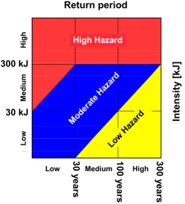
Following the Swiss Federal Guidelines (OFAT, OFEE, OFEFP, 1997; Raetzo et al., 2002), the hazard analysis has been made by taking into account the two parameters intro-duced in the previous section. The first is the rock fall inten-sity, expressed by the total kinetic energy (translational and rotational) of the falling blocks, which is obtained by rock fall trajectory simulations. The other is the return period, de-fined as the mean reference time within which a rock fall may occur (inverse of the mean rock fall frequency). According to a matrix diagram combining intensity and return period (Fig. 1), the rock fall hazard was classified into three levels: low, moderate, and high.
J. M. Abbruzzese et al.: Considerations on Swiss methodologies for rock fall hazard mapping 1097
28
801
Return period
Intensi
ty
[kJ
]
30 y
e
ar
s
100 y
ears
300 y
e
ar
s
Low Medium High
Hi
gh
Mediu
m
Low
High Hazard
Mod erat
eHa zard
Low Haza
rd
300 kJ
30 kJ
Return period
Intensi
ty
[kJ
]
30 y
e
ar
s
100 y
ears
300 y
e
ar
s
Low Medium High
Hi
gh
Mediu
m
Low
High Hazard
Mod erat
eHa zard
Low Haza
rd
300 kJ
30 kJ
802
Figure 1. Swiss intensity-frequency diagram (from OFAT, OFEE, OFEFP, 1997).
803
804
805
806
807
808
Figure 2. Modified Matterock methodology: cumulative distribution of the blocks energy at a
809
given abscissa. The energy profile along the slope is evaluated by taking into account, at each
810
abscissa, the energies of only 90% of the simulated blocks.
811
812
0 40 60
0 100 200 300 400 500
20 80
P [%]
100
E [kJ]
Fig. 1. Swiss intensity-frequency diagram (from OFAT, OFEE,
OFEFP, 1997).
according to the Swiss guidelines that are documented in published reports (Rouiller et al., 1998; Jaboyedoff and Labi-ouse, 2002): the Matterock and the Cadanav procedures.
2.1 The Matterock methodology
2.1.1 Matterock methodology: original approach
The Matterock methodology (Rouiller and Marro, 1997; Rouiller et al., 1998) was proposed in the Canton of Valais for the detection of rock fall prone areas. In order to pro-duce a hazard map, the study of the potential rock fall source areas must be coupled with the performance of 2D rock fall trajectory simulations. For obtaining the hazard at a given point on a slope according to the matrix diagram proposed by the Swiss Guidelines (Fig. 1), the Matterock methodol-ogy evaluates the probability of occurrence as the result of the combination between the probability of mobilisation of a block and the probability that, once detached, this block reaches a given point along the slope (probability of reach).
The probability of mobilisation is defined in a qualitative way, by a detailed study of the potential rock fall departure areas, which are assigned a score, depending on the pattern of the discontinuity sets and on the presence of instability fac-tors: continuity of the joints sets, degree of activity (rock fall history), presence of water, sensibility to degrading factors (weathering, micro-seismicity, freeze and thaw cycles) and to triggering factors (earthquake, heavy rainfalls), “safety fac-tor” (based on structural/geomechanical features and expert’s qualitative estimation). As a function of the obtained score, three levels of probability of mobilisation are defined: low, moderate and high.
Table 1. Matterock methodology: definition of the probability of
occurrence.
Probability of occurrence Probability of mobilisation
high moderate low
Probability of reach
high high moderate low
moderate moderate low –
low low – –
The probability of reach is evaluated by trajectory simula-tions from the distribution of the blocks deposited along the slope. More precisely, three “propagation limits” are defined to classify this probability into high, moderate or low. These limits correspond to the abscissas passed by 10−2, 10−4and 10−6of the blocks with respect to the total number of com-puted trajectories (or 1, 10−2and 10−4if expressed in per-cent).
Finally, as shown in Table 1, the probability of mobilisa-tion and the probability of reach are coupled to obtain a qual-itative estimate of the probability of occurrence, which can also be classified as high, moderate or low. The kinetic en-ergy is determined by means of trajectory simulation results. The analysis of the energy profile along the slope allows the definition of a low, moderate or high intensity, according to the 30 kJ and the 300 kJ thresholds of the diagram. Once in-tensity and probability are known at each point of the slope, the hazard level is obtained by checking which zone of the diagram (red, blue or yellow) corresponds to the considered intensity-probability couple at that location.
2.1.2 Matterock methodology: modified approach cur-rently used in the Canton of Valais
The most significant modification of the Matterock approach concerns the number of blocks being used when evaluat-ing the kinetic energy. The energy profile mentioned in Sect. 2.1.1 is an envelope of the maximum energy of all the simulated blocks. In this modified approach, on the contrary, only a percentage of the total number of simulated blocks is considered to estimate the energy profile value at each point of the slope. The chosen percentage is fixed to 90% in the Canton of Valais. This step is made to avoid taking into account the maximum values of the energy obtained by the computations, which could determine, on one hand, ex-treme unfavourable conditions for the hazard mapping and, on the other hand, very high costs in the design of protective measures. In the latter case, with the proposed method, the protective measures will be less costly, but nevertheless be able to guarantee a sufficient degree of protection. Figure 2 shows how the energy corresponding to 90% of the blocks propagating down slope is determined from the cumulative distribution of the energy computed at a given abscissa.
1098 J. M. Abbruzzese et al.: Considerations on Swiss methodologies for rock fall hazard mapping
28
801
Return period
Intensi
ty
[kJ
]
30 y e ar s 100 y ears 300 y e ar sLow Medium High
High Mediu m Low High Hazard Mod erat
e Haz ard Low Haza rd
Return period
Intensi
ty
[kJ
]
30 y e ar s 100 y ears 300 y e ar sLow Medium High
High Mediu m Low High Hazard Mod erat
e Haz ard
Low Haza
rd
802
Figure 1. Swiss intensity-frequency diagram (from OFAT, OFEE, OFEFP, 1997).
803
804
805
806
807
808
809
810
811
812
813
Figure 2. Modified Matterock methodology: cumulative distribution of the blocks energy at a
814
given abscissa. The energy profile along the slope is evaluated by taking into account, at each
815
abscissa, the energies of only 90% of the simulated blocks.
816
817
0 40 60
0 100 200 300 400 500
20 80 P [%]
100
E [kJ]
Fig. 2. Modified Matterock methodology: cumulative distribution
of the blocks energy at a given abscissa. The energy profile along the slope is evaluated by taking into account, at each abscissa, the energies of only 90% of the simulated blocks.
2.2 The Cadanav methodology
The Cadanav methodology (Jaboyedoff and Labiouse, 2002) has been developed by the Rock Mechanics Laboratory of EPFL, for producing rock fall hazard maps for the Canton of Vaud. This methodology (here presented in 2-D), however, has not yet been applied.
The hazardH (E, x)at an abscissax is expressed as the product between the mean frequency of failureλf of a rock
mass, the number of blocksNblocksdetaching from the cliff in a single event and the probability of propagationPp(E, x),
that is, the probability that a block reaches a selected area with a given intensityE(Jaboyedoff et al., 2005):
H (E, x)=λf ·Nblocks·Pp(E, x) (1)
At first, an annual frequency of failure λf of the unstable
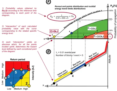
rock mass has to be evaluated from available historical data collected via rock fall inventories (Dussauge-Peisser et al., 2002; Hantz et al., 2003; Corominas and Moya, 2008). From the persistence and spacing characterising the main joint sets, a “reference block” can be defined, whose size is chosen as the most representative for the potential rock fall source area and will be considered for the trajectory modelling. After the estimation of the volume of the whole event, the total volume is divided by the reference block size to obtainNblocks. Then, the distribution of the kinetic energy along the slope is com-puted by means of rock fall trajectory simulations. For each simulated block (for each trajectory) the real energy profile is modified defining the points where the threshold values pro-posed by the Swiss Guidelines (0, 30, 300 kJ) are reached for the last time, and assigning that energy value to all the points located “upslope” (Jaboyedoff et al., 2005). This step is rec-ommended for land-use applications, to ensure in every map that the hazard level decreases downslope.
From the modified energy profiles, propagation proba-bility curvesPp(E, x) are then drawn for the fixed energy
thresholdsEof 0, 30, 300 kJ. Three curves are obtained by
analysing the cumulative frequency of the blocks that reach a particular abscissaxalong the profile, with a given energy valueE(Fig. 3).
The limits of the hazard zonesxEiare determined by
eval-uating where the probability that a block reaches a certain abscissa with a given energyEi is lower than 1 over a
spec-ified period of time. For an assigned reference timetref, the abscissa where this condition is fulfilled is found for a prob-ability of propagation of:
Pp(Ei, xEi)=
1 λf ·tref·Nblocks
(2) By using the probability curves, relatingPpandx,xEican be
determined, for each intensity-frequency couple (according to the Swiss Guidelines), as the abscissa beyond which the probability of propagation is lower than the calculated value Pp(Ei, xEi)(Fig. 3). The limit of each hazard zone is then
traced by considering the most unfavourable case among the different intensity-frequency couples, which is represented by the one giving the highest downhill abscissa. Further de-tails on this methodology are available from Jaboyedoff et al., 2005).
3 Application of the methodologies to a study area in the Canton of Valais (Switzerland)
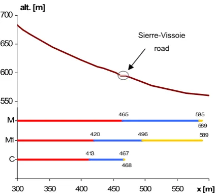
The presented hazard mapping methodologies (original and modified Matterock, Cadanav) are compared in a case study in the Canton of Valais, in Switzerland. The site is the Creux de Chippis (Fig. 4), whose cliffs are constituted by dolomitic limestone and Triassic gypsum. The structure of the rock mass is characterised by three main discontinuity sets; the persistence varies between 0.5 m and 10 m and the spacing between 0.05 m and 0.5 m. The hazard zoning is performed along a selected slope profile, identified as P2, which starts from an elevation of 900 m to end at 550 m (Fig. 4). The de-parture zone is characterised by blocks ranging from 0.5 to 1.0 m3 in size. Two “extreme blocks” (in terms of longer propagation) can be observed on site, close to the chosen profile; they both stop close to a road, which is one of the primary assets threatened by rock falls in this area.
The hazard analysis for the chosen profile is based on the geological field survey data and on the computer simula-tion results performed by the Geological firm G´eoval. From the geological study, a size of 1.0 m3was defined to charac-terise the potentially unstable “reference” blocks, following the procedure explained in Sect. 2.2 (basically no other vol-ume was considered as important for running the computer simulations). The rock fall simulations were performed with the Rockfall 6.0 code (Spang and Krauter, 2001). The num-ber of runs was set up to 300, based on the procedure cur-rently practiced in Valais.
J. M. Abbruzzese et al.: Considerations on Swiss methodologies for rock fall hazard mapping 1099
29
813
814
815
816
Figure 3. Cadanav methodology. Scheme of determination of the hazard zone limits (after
817
Jaboyedoff et al., 2005). The example shows events of 5 blocks with a mean frequency of
818
failure of 1 event over 100 years. The probability of 7% is related to points 2 and 7
819
corresponding to a reference time of 300 years.
820
821
822
823
824
825
826
827
3) each “intersection” yields an abscissa which, for all the points located uphill, determines the hazard level defined by each considered point of the diagram.
2) “intersection” of each calculated probability value with the curve corresponding to the related specific energy level.
1) Probability values obtained by Eq.(2) according to the reference time corresponding to each point of the diagram.
E>0kJ
Fig. 3. Cadanav methodology. Scheme of determination of the hazard zone limits (after Jaboyedoff et al., 2005). The example shows events
of 5 blocks with a mean frequency of failure of 1 event over 100 years. The probability of 7% is related to points 2 and 7 corresponding to a reference time of 300 years.
30 827
828
829
830
Figure 4. Left: location of the Creux de Chippis area (source: Swisstopo). The site is close to 831
the town of Sierre, Canton of Valais. Right: the profile chosen for the present study (P2). 832
833
834
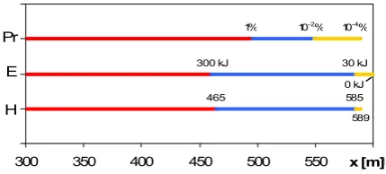
H 465 585589
300 kJ 30 kJ
0 kJ
Pr 10
-2%
1% 10-4%
300 350 400 450 500 550 x [m]600
E
835
836
Figure 5. Matterock Methodology: procedure for obtaining the hazard (H), according to the 837
Swiss diagram shown in Figure 1, once probabilities of reach (Pr) and energies (E) are known 838
for a defined class of probability of mobilisation (fixed as “high” in this application). 839
500 600 700 800 900
0 100 200 300 400 500 x [m]600 alt. [m]
departure zone
bedrock/ rock deposits
7 m3 1 m3 Sierre-Vissoie
road
soil covered by blocks 500
600 700 800 900
0 100 200 300 400 500 x [m]600 alt. [m]
departure zone
bedrock/ rock deposits
7 m3 1 m3 Sierre-Vissoie
road
soil covered by blockssoil
P2 Profile P2 Profile
Fig. 4. Left: location of the Creux de Chippis area (source: Swisstopo). The site is close to the town of Sierre, Canton of Valais. Right: the
profile chosen for the present study (P2).
1100 J. M. Abbruzzese et al.: Considerations on Swiss methodologies for rock fall hazard mapping
H 465 585589
300 kJ
0 kJ 30 kJ
Pr 1% 10
-2% 10-4%
300 350 400 450 500 550 x [m]600
E
1
Fig. 5. Matterock Methodology: procedure for obtaining the hazard
(H), according to the Swiss diagram shown in Fig. 1, once proba-bilities of reach (Pr) and energies (E) are known for a defined class of probability of mobilisation (fixed as “high” in this application).
the Matterock and Modified Matterock methodologies and choosing a 1 year return period for Cadanav (which fulfils the need of the method of assigning a quantitative value to this parameter and considers the most unfavourable condi-tions in terms of frequency).
The zoning procedure is applied under the hypothesis of an infinite linear cliff with a planar slope topography below, which in reality is representative of many topographical set-tings, though it is quite a simplified model. The results are, therefore, shown only with reference to the selected 2-D pro-file.
3.1 The Matterock methodology
The hazard is determined from the rock fall kinetic energy along the slope and the probability of occurrence. From the envelope of maximum energy, obtained directly from trajec-tory simulations, the abscissas corresponding to the 300 kJ and the 30 kJ threshold values can be determined. The energy is high up to the 460 m abscissa, intermediate up to 585 m and low farther along the slope (Fig. 5).
For the probability of occurrence, the probability of mo-bilisation is fixed as “high” and the abscissas corresponding to high, moderate and low probabilities of reach have to be determined (Table 1). The simulation of 300 runs does not allow the abscissas corresponding to the propagation of 10−4 and 10−6of the blocks to be determined. A statistical extrap-olation of the computed deposit zones is therefore necessary to get these points. For this purpose, a normal distribution is assumed to correctly fit the data coming from the computer runs. Once mean and standard deviation of the computed run-outs are calculated, it is possible to derive the abscissas by using the chosen distribution law for the probability val-ues of 10−2, 10−4and 10−6. Then, from Table 1, it is possible to evaluate the probability of occurrence. It is high above the 496 m abscissa, moderate up to 549 m and low up to 589 m (Fig. 5).
The hazard zoning is performed using the intensity-frequency diagram shown in Fig. 1 in which the intensity-frequency (probability of mobilisation) is already coupled with the
probability of propagation of the blocks along the slope. This means that the probability of occurrence is actually the pa-rameter on the horizontal axis that is afterwards combined with the energy. Despite all the essential information being available, it is still possible that the evaluation of the hazard is not straightforward: i.e. some zones of the diagram are char-acterised by two possible levels of hazard. A further check is then necessary to determine whether the energy-probability couple is located above or under the diagonal. The appropri-ate hazard level can be chosen without ambiguity by writing the equation of the diagonal. Since both the probability of propagation value and the envelope of the maximum energy are known at each point of the slope, the equation of the diag-onal allows a check on which hazard level corresponds to the considered couple, according to its location above or under the diagonal. Figure 5 shows the resulting hazard mapping along the studied profile. The red, blue and yellow colours are associated with the high, moderate and low hazard levels, respectively.
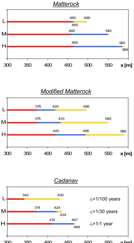
3.2 The Modified Matterock methodology
The mapping performed with this approach is similar to the previous one, except for the modification of energy already explained in Sect. 2.1.2: i.e. 90% of the simulated blocks are considered to obtain the energy profile along the slope. Therefore, the abscissas corresponding to the 300 kJ and 30 kJ threshold values are uphill with respect to those de-termined by the original Matterock methodology, and the re-sulting hazard mapping is less conservative (Fig. 7). 3.3 The Cadanav methodology
To apply the Cadanav methodology, it is first necessary to es-timate the temporal frequency of failureλf and the number
of detaching blocks from a historical catalogue. For this ex-ample, a return period of 1 year was considered (according to the hypothesis of high frequency of failure) and the release of only one block per event was assumed (Nblocks=1).
From trajectory simulation results it is possible to draw probability curves for each energy threshold of the Swiss Guidelines (0, 30, and 300 kJ), as follows. For an energy threshold, e.g. 30 kJ, the abscissa where a simulated block reaches for the last time that threshold is determined, for each computed run (300, in this case). Then, by ordering these data, it is possible to determine for all the calculated abscissas how many blocks will reach an energy higher than 30 kJ downhill (along with the corresponding value in per-centage). The resulting set of 300 “cumulative frequency-abscissa” couples is used to draw the curve. The same pro-cedure is repeated for all the three energy thresholds.
J. M. Abbruzzese et al.: Considerations on Swiss methodologies for rock fall hazard mapping 1101
31 840
841
842
Figure 6. Scheme of determination of the hazard limits in Cadanav (as in Figure 3). Above: 843
shape of the three probability curves for the studied example. Below: use of the intensity-844
frequency couples to obtain the hazard zone limits. The red, bright blue and yellow points of 845
the diagram define the three abscissas representing the high, moderate and low hazard zone 846
limits respectively, following the procedure illustrated in Figure 3. 847
848
849
850
851
852
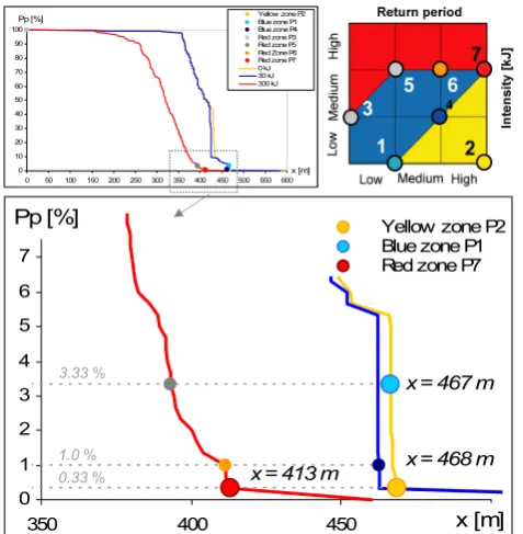
x = 413 m x = 468 m x = 467 m
0 1 2 3 4 5 6 7 8
350 400 450 x [m]500
Pp [%] Yellow zone P2
Blue zone P1 Red zone P7
0.33 %
1.0 %
3.33 % 0
10 20 30 40 50 60 70 80 90 100
0 50 100 150 200 250 300 350 400 450 500 550 600 x [m] Pp [%] Yellow zone P2Blue zone P1
Blue zone P4 Red zone P3 Red zone P5 Red Zone P6 Red zone P7 0 kJ 30 kJ 300 kJ
Fig. 6. Scheme of determination of the hazard limits in Cadanav
(as in Fig. 3). Above: shape of the three probability curves for the studied example. Below: use of the intensity-frequency couples to obtain the hazard zone limits. The red, bright blue and yellow points of the diagram define the three abscissas representing the high, moderate and low hazard zone limits respectively, following the procedure illustrated in Fig. 3.
reference time is lower than 1. For instance, for events with a return period of one year (λf=1) and a single block release
(Nblocks=1), the abscissas beyond which the probability of occurrence over a 100 year period (tref)is lower than 1 are found for a probability of propagation of 1/100=1%, i.e. at 411 m, 462 m and 467 m for the 300 kJ, 30 kJ and 0 kJ en-ergy threshold values, respectively.
The abscissas representing the hazard zone limits are de-termined considering the energy-frequency couples of the di-agram which mark a change between different hazard levels (points from 1 to 7 in Fig. 6). As an example, the yellow point (2) associated to a 0 kJ energy threshold and to a 300 year ref-erence time determines the extension of the yellow zone (low hazard). The 300 year reference time is used in Eq. (2) for calculating the correspondent propagation probability value (Pp=1/300=0.33%). The yellow zone limit is therefore found
by determining, on the 0 kJ curve, which abscissa corre-sponds to the propagation probability value of 0.33%. The same procedure is repeated for all the seven points, and when more than one point can define the limit between two haz-ard levels, the one giving the most unfavourable conditions is chosen (i.e. the point yielding the largest extent of the hazard zone). In Fig. 6, the abscissasx=413 m, x=467 m andx=468 m delineating the red, blue and yellow zones
cor-respond respectively to point 7 (red point), point 1 (bright blue point) and point 2 (yellow point). Figure 7 represents the corresponding hazard mapping obtained by the Cadanav methodology, together with those drawn from the original and modified Matterock methodologies.
3.4 Results
The zoning performed according to the three approaches pro-duces rather different results (Fig. 7). In particular, the Mat-terock methodology generates a larger spatial extent of the hazard zones, if compared to Cadanav. This is a consequence of the application of a normal distribution (in Matterock) for extrapolating the computed runout points and determin-ing the abscissas corresponddetermin-ing to very low probabilities of reach (10−2, 10−4and 10−6). Due to the extrapolation, the portion of the slope potentially reached by blocks becomes actually larger than the one obtained directly from the com-puted runout points, without any statistical processing. This, in turn, influences the determination of the hazard zone lim-its (as it also comes out by analysing the mapping scheme in Fig. 5).
The same observations can be made by comparing the “modified” Matterock methodology and Cadanav. In this case, however, the biggest difference concerns mainly the limit of the yellow zone, as there is almost no change for the red zone and only a 20 m change for the blue zone. The method for estimating the energy in the Modified Matterock explains differences in the hazard zoning with respect to Mat-terock. In the latter methodology, one or some blocks char-acterised by a longer propagation influence the extent of the hazard zones not only in terms of probabilities of reach, but also because the energy profile changes (basically: the higher the energy, the higher the hazard). On the other hand, in the former approach, by taking 90% of the blocks to estimate the energy profile, the hazard zone limits determined by the rock fall intensity are not influenced anymore by such blocks with a longer propagation. The limits of the red and blue zones are therefore much more similar to those obtained with the Cadanav approach.
The results discussed so far give evidence that some issues need to be kept in mind during the hazard mapping process, because they can considerably affect the hazard assessment:
– First, an assumption of “high” frequency of failure has been made. It is now important to study what happens in terms of hazard mapping if a change in this factor occurs (e.g. uncertainty in the estimation of the rock fall frequency or need to update the hazard map when triggering factors change), especially considering that the way it is evaluated differs depending on the applied methodology.
– Furthermore, the application of the Matterock method-ology introduces the question of assessing which role
1102 J. M. Abbruzzese et al.: Considerations on Swiss methodologies for rock fall hazard mapping
32
853
854
Figure 7. Results of the hazard mapping performed with the Matterock (M), Modified
855
Matterock (M1) and Cadanav (C) methodologies (the mapping shows the profile abscissas
856
located between 300 and 600 m. From
x
=0 m to
x
=300 m the obtained hazard level is “high”
857
for all the methodologies).
858
859
860
861
862
863
864
865
866
867
868
869
870
871
M 465 585
589
M1 420 496 589
C 413 467
468
300 350 400 450 500 550 x [m]600
550 600 650 700 alt. [m]
Sierre-Vissoie road
Fig. 7. Results of the hazard mapping performed with the
Matte-rock (M), Modified MatteMatte-rock (M1) and Cadanav (C) methodolo-gies (the mapping shows the profile abscissas located between 300 and 600 m. Fromx=0 m tox=300 m the obtained hazard level is “high” for all the methodologies).
the longer propagation of a few blocks predicted in the computation plays on the final mapping.
– As the prediction of “extreme blocks” (longer propaga-tion) is related to the random character of the modelling parameters (e.g. restitution coefficients) considered in many rock fall codes, it is expected that several simula-tions will not provide the same trajectory results. Does this have an influence on hazard mapping?
The next section is dedicated to the analysis of all these as-pects.
4 Parametric study
4.1 Influence of a change in the temporal frequency of failure
The definition of hazard features a “time dependency”, which concerns the frequency of failure and the propagation of the event. Taking into account the frequency of failure of a rock mass allows a description of the evolution of the hazard level due to changes in triggering factors. On the other hand, un-fortunately, the rock fall frequency can not be correctly in-vestigated if there are no inventories of historical data and/or information about past events (“scars” on the cliff, traces on the slope, impacts on trees in forested slopes). Consequently, a potential lack of accuracy may affect quantitative method-ologies which take into account the temporal frequency of failure of rock falls (in terms of number of blocks per event and return period), as for instance Cadanav does. For this
reason, some methodologies like Matterock propose a quali-tative estimate of this parameter. The problem, in this case, is the subjectivity which affects the judgement when evaluating this probability.
In this section, the influence of a change in rock fall fre-quency on hazard mapping is analysed. A first application shows the results of a change in the rock fall frequency by assuming different return period values for the same event studied in Sect. 3. A second example of zoning is then per-formed, taking into account a change in the block volume and in the related return period.
4.1.1 Change in the event frequency of failure
As for Matterock and Modified Matterock, a change in the probability of mobilisation is taken into account. The zoning is performed for a “high”, a “moderate” and a “low” proba-bility of mobilisation. In the case of Cadanav, according to the return periods proposed by the Swiss Guidelines, mean rock fall frequencies of 1 block every year, 1 block every 30 years and 1 block every 100 years have been considered to assess the hazard.
Figure 8 shows the results obtained by the three method-ologies. As expected, the higher the rock fall frequency is, the larger the areas in danger. The limits of the hazard zones move down slope as the frequency of failure increases, for all the three mapping approaches. Compared to Cadanav, the larger extent of the hazard zones resulting from Matte-rock (original and modified methodologies) is again due to the very low probabilities of reach and to the statistical anal-ysis these methods consider.
4.1.2 Change in block volume and related frequency of failure
Large boulders are frequently found to propagate beyond the main deposit zone. Due to their longer runout and higher in-tensity, these blocks constitute a significant hazard that has to be taken into account. Uncertainty about the return pe-riod of such rock fall events poses however a major difficulty for the hazard mapping. On the site of interest, the lack of rock fall historical inventories and of detailed collected data on fragments sizes on the talus (Evans and Hungr, 1993) did not allow the determination of a return period related to the block volume. Events with a single block of 5 m3 volume were considered and assumed to have a “moderate” proba-bility of mobilisation, according to both the Matterock and Modified Matterock methodologies. For Cadanav, the cho-sen return period was equal to 30 years, based on the same considerations explained in the previous example (Sect. 3).
J. M. Abbruzzese et al.: Considerations on Swiss methodologies for rock fall hazard mapping 1103
33
872
873
Figure 8. Influence of a change in rock fall frequency on hazard mapping. The results are
874
obtained by varying the probability of mobilisation
Pr
in Matterock and Modified Matterock
875
(low “L”, moderate “M” and high “H”) and the rock fall frequency in Cadanav (“L”= 1 block
876
every 100 years, “M”= 1 block every 30 years, “H”=1 block every year).
877
878
879
880
881
882
Cadanav
H 413 467468
M 374 424
434
L 343 430
300 350 400 450 500 550 x [m]600
λf=1/100 years
λf=1/30 years
λf=1/1 year Matterock
H 465 585
589
M 460 549
L
465 460 496
300 350 400 450 500 550 x [m]600
Modified Matterock
H 420 496 589
M 375 433 549
L 375 420 496
300 350 400 450 500 550 x [m]600
Fig. 8. Influence of a change in rock fall frequency on hazard
map-ping. The results are obtained by varying the probability of mobili-sation Pr in Matterock and Modified Matterock (low “L”, moderate “M” and high “H”) and the rock fall frequency in Cadanav (“L”= 1 block every 100 years, “M”= 1 block every 30 years, “H”=1 block every year).
for the case of “moderate” frequency (M) in Fig. 8 (1 m3) with the results reported in Fig. 9 (5 m3).
Due to the higher energy characterising the propagation of the 5 m3blocks, all the methodologies provided a larger ex-tent downhill of the red and blue zones. This is also the case for the yellow zone obtained with the Cadanav methodol-ogy. On the contrary, in Matterock and Modified Matterock an astonishing trend can be observed, which shows the yel-low zone moving uphill when compared to the zoning rep-resented in Fig. 8. Since the determination of this limit is not strongly affected by the energy values but mostly by the runout points reached by the blocks, the location and the pat-tern of the block deposit zones along the slope play a
ma-M 516 519
523
M1 394 467 523
C 462
467
300 350 400 450 500 550 x [m]600
1
Fig. 9. Influence of a change in the block size and related return
period on hazard mapping.
jor role in defining the extension of the low hazard area. In the 5 m3simulation the points where the blocks stop are less scattered than the ones of the 1 m3 simulation. Therefore, the normal distribution used to fit them has a smaller stan-dard deviation and the abscissas corresponding to the proba-bilities of reach of 10−2, 10−4and 10−6are positioned more uphill. From this, it comes out that, for the Matterock and Modified Matterock methodologies, there is a certain degree of uncertainty in the obtained mapping results related to the statistical procedures used for computing the limits of reach. Considering the influence that a statistical extrapolation has on the final result, if a normal (or other) distribution is as-sumed to correctly fit the deposition zone of the blocks, this assumption must be justified by performing statistical tests to verify the eventual match between the data and the con-sidered distribution law.
Finally, it can be noted that the blue zone is vanishing in Cadanav. This situation happens generally with large boul-ders and/or long return periods, when the extent of the blue and red zones coincide, i.e. when both limits are defined by the triple point of the Swiss intensity-frequency matrix cor-responding to an energy of 300 kJ and a return period of 300 years (Fig. 1).
4.2 Influence of “extreme blocks” predicted by com-puter simulations
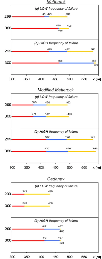
As previously introduced, the longer propagation of one or more blocks much farther than the main deposit zone may influence the hazard mapping, depending on the particular methodology. This influence is investigated for all three ap-proaches. Since the simulation of 300 blocks shows the pres-ence of only 1 block travelling much farther than the others, the results here presented illustrate the hazard mapping ob-tained by the 300 run simulation and by a 299 run simulation, derived from the previous one just by “removing” the result related to the block stopping way beyond the others.
This issue aims at discussing the problem of how to treat this type of results. Indeed they may describe possi-ble, though probably rare, rock fall paths (with their con-sequences on hazard) or be results not corresponding to re-ality. And in case one intends to consider these results, is
1104 J. M. Abbruzzese et al.: Considerations on Swiss methodologies for rock fall hazard mapping it relevant to have a hazard map influenced by such a little
number (or just one, in this case) of runs with respect to the general “trend” of the whole simulation?
Figure 10 shows the mapping obtained by the three methodologies, by using 299 and 300 runs simulations in the cases of “high” and ”low” frequency of failure. It is quite evident that the influence of extreme runout distances is strong in Matterock when compared to Modified Matte-rock and Cadanav. Actually, in Cadanav, the use of proba-bility curves ensures that a “single” result has no importance in the whole mapping process, in terms of both propagation and energy of the blocks. Actually, there is no difference be-tween the mapping coming from the 299 and the 300 runs simulations, for both the considered values of the frequency of failure.
This last statement is also valid for the Modified Matterock methodology, for which the energy profile obtained by con-sidering 90% of the simulated blocks allows to limit the in-fluence of some of them which, due to higher energies, have a longer propagation on the slope. Only a small difference in mapping results is noted.
In the original Matterock methodology, on the contrary, since all the results are taken into account, including the ones defined as “extreme”, a single block can change a lot the final mapping. Particularly, it is clear that the limits of the zones characterised by higher levels of hazard (red and blue) move down slope when the extreme block result is taken into ac-count. If the original Matterock methodology is applied, it would then be important to decide whether to consider such a kind of result or not.
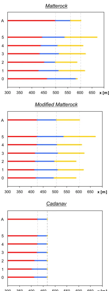
4.3 Influence of the number of runs performed in rock fall simulations
The problem analysed in the previous section introduces an-other issue to account for when hazard mapping is performed by means of trajectory simulations results. Since most tra-jectory codes are characterised by a stochastic approach, as-signing to the input parameters random values taken from specified intervals, it can’t be expected to get the same re-sults when more than one simulation is performed (except if a seed-based pseudo-random sampling is used by the code). This may have an influence on the extent of the hazard zones. Consequently, in addition to the one already analysed, five more simulations of 300 runs were carried out to assess the hazard mapping variability for the three methodologies. The results are represented in Fig. 11 for a “high” probabil-ity of mobilisation, for the original and modified Matterock methodologies, and for a mean frequency of 1 block per year for Cadanav.
The results show that Cadanav is again the less sensitive methodology, also to this factor. The limits of the blue and yellow zones do not change at all, and the limit of the red zone is affected by a small variation of about 23 m over the considered slope length of 600 m.
35 Matterock
Cadanav Modified Matterock
300 460
465 496
299 413 429 492
300 465 585
589
299 429 492 581
300 350 400 450 500 550 x [m]600
300 343 430 299 343 430
300 413 467
468
299 412 467
468
300 350 400 450 500 550 x [m]600
300 375 420 496 299 375 420 492
300 420 496 589
299 420 492 581
300 350 400 450 500 550 x [m]600
(b) HIGH frequency of failure
(a) LOW frequency of failure
(b) HIGH frequency of failure
(a) LOW frequency of failure
(a) LOW frequency of failure
(b) HIGH frequency of failure 905
906
907 908 909 910 911 912 913 914 915 916 917 918 919 920 921 922 923 924 925 926 927 928 929 930 931 932 933 934
Figure 10. Influence of the extreme runout of a block on hazard mapping. The 299 run case 935
does not take into consideration the block with longer runout, while the 300 run case does. 936
The results are presented for two different values of the frequency of failure. (a) For the 937
Fig. 10. Influence of the extreme runout of a block on hazard
J. M. Abbruzzese et al.: Considerations on Swiss methodologies for rock fall hazard mapping 1105
37 943
Figure 11. Influence of the number of simulation runs on hazard mapping. Number “0” refers 944
to the 300 run simulation discussed in Section 3. The numbers from 1 to 5 indicate the other 945
performed 300 run simulations. The letter “A” refers to the additional 10’000 run simulation 946
used for the comparison with the 300. 947
Matterock
300 350 400 450 500 550 600 650 x [m]700
5
4
3
2
1
0 A
Modified Matterock
300 350 400 450 500 550 600 650 x [m]700
5
4
3
2
1
0 A
Cadanav
300 350 400 450 500 550 600 650 x [m]700
5
4
3
2
1
0 A
Fig. 11. Influence of the number of simulation runs on hazard
map-ping. Number “0” refers to the 300 run simulation discussed in Sect. 3. The numbers from 1 to 5 indicate the other performed 300 run simulations. The letter “A” refers to the additional 10 000 run simulation used for the comparison with the 300.
As for Modified Matterock, the variation in the red zone limit is still comparable to the one obtained by Cadanav (even smaller: 16 m), but the variation characterising the extension of the blue and yellow zones is much higher, reaching 42 m and 83 m, respectively.
According to what has been observed so far, the Matterock methodology is the one presenting the most noticeable vari-ability concerning this issue. The variation of the red zone limit is 31 m, while the blue zone limit shows a maximum variation of 39 m, among the new five simulations, and even of 86 m when also the first simulation is taken into account. Finally, the yellow zone is also affected by a remarkable vari-ation, whose maximum value is 83 m.
In order to reduce as much as possible the variability of the trajectory results from one simulation to another, and conse-quently of hazard mapping, an increase in the number of runs within a single simulation has been considered. For this pur-pose, as the maximum capability of the Rockfall 6.0 code in terms of runs in a single simulation is 10 000, a 10 000 runs simulation was carried out (case A in Fig. 11). Com-paring the hazard mapping provided by this last computa-tion (which can be considered as more reliable because of the higher number of runs) with the 300 runs simulations ones, it comes out once again that only Cadanav seems to be not highly dependent on the number of performed calculations (small or null variations of the hazard zone limits).
5 Discussion
The rock fall hazard mapping procedures presented in this work lead to considerable differences in the final results. De-spite all of them being based on the Swiss Federal Guide-lines, some uncertainties in the methodologies and the pe-culiar way each approach interprets the Swiss intensity-frequency diagram do not produce a good agreement in the overall zoning. Clearly, the fact that three methodologies (or, at least, two different approaches) provide potential users with different rock fall hazard maps is very questionable, since these maps are meant to be a basic document for land-use planning.
5.1 Matterock versus Cadanav
As for differences in the interpretation of the matrix diagram, Matterock does not actually combine the energy and proba-bilities of occurrence data. They are processed separately. The probabilities of reach and then of occurrence (i.e. prod-uct of the probabilities of mobilisation and of reach accord-ing to the Matterock methodology) are estimated only refer-ring to the deposit zones of the blocks, but with no “refer-ence” to the energy (particularly to the threshold values of the Guidelines). Then, the energy profile is simply “super-imposed” onto the probability of occurrence (Fig. 5).
In Cadanav, the probability that a detached block can reach a given abscissa in a given reference time is defined depend-ing on the energy. As explained, the probability curves are drawn for specified energy thresholds, which are coupled in turn with the return periods (Figs. 3 and 6). The abscis-sas corresponding to the different points 1 to 7 of the Swiss
1106 J. M. Abbruzzese et al.: Considerations on Swiss methodologies for rock fall hazard mapping intensity-frequency matrix are determined by the intersection
of:
– the probability curves obtained for the energy thresholds of 0, 30 and 300 kJ;
– the horizontal lines traced for the reference times of 30, 100 and 300 years, and accounting for the annual fre-quency of triggered blocks (see Eq. 2).
Indeed, the two approaches are really different, and conse-quently it may not be surprising that different results arise, even though there is a common base to the evaluation of the hazard.
Additionally, Matterock needs some threshold values for the probability of reach (abscissas of propagation of 10−2, 10−4and 10−6of the simulated blocks): if these values were different, the resulting hazard mapping would differ as well. As for Cadanav, the modification of the energy profiles explained in Sect. 2.2 produces a more straightforward cou-pling of energy and return periods in the estimation of the rock fall hazard, but on the other hand it can only provide a single sequence of hazard levels decreasing down slope. Thus, this procedure does not account for possible “inverse zoning” (i.e. areas of higher hazard located after areas char-acterised by lower hazard). This feature may appear in haz-ard maps if, for instance, due to the slope topography, blocks could regain energy. This issue, which was not encountered in the case study presented, may be significant for land-use applications at a given site.
The characterisation of potentially unstable source areas and the assessment of the frequency of occurrence are among the most difficult tasks in the hazard mapping process. They involve much uncertainty and judgement and consequently it is common practice to report their likelihood using qualita-tive terms (AGS, 2002), such as in the Matterock methodol-ogy: low, moderate and high probability of mobilisation. A review of the methods available to estimate the frequency of events was compiled by the Australian Geomechanics So-ciety (AGS, 2002) based on Mostyn and Fell (1997) and Baynes and Lee (1998). In the best case, when a historic record of rock falls occurring on the site of interest is avail-able, a relationship can be worked out between the magnitude of the events and their frequency of occurrence (Hungr et al., 1999; Dussauge at al., 2002; Hantz et al., 2003; Chau et al., 2003). Though discussing this issue is not an aim of this pa-per, this aspect must be taken into account when performing hazard analyses. The Cadanav methodology allows this, by introducing the number of released blocks in a single rock fall event in the definition of the hazard (Eq. 2): once the rock fall volume and the “reference block” size are known, a change in the event’s volume can be accounted for by chang-ing the number of blocksNblocks.
Different block sizes should also be taken into account when modelling rock fall propagation because block size has
a major influence on energy and runout distances. The in-fluence of block size can be taken into account by running simulations where different block sizes can be accounted for or by defining several scenarios and running different simu-lations for different block sizes.
Finally, the results presented in this paper are obtained by hazard analyses performed for very specific events. In the hazard zoning comparison related to different block sizes, discussed in Sect. 4.1.2, it was implicitly assumed that ei-ther a rock fall of 1 m3or one of 5 m3may occur. Actually, when more than one instability can affect a given site, hazard assessment procedures must include all the possible events that can occur. Consequently, the hazard maps have to repre-sent the hazard resulting from the combined effects of all the sources of instability (Jaboyedoff et al., 2005).
5.2 Swiss guidelines
Another issue concerning the intensity-frequency matrix pro-posed by the Swiss Guidelines involves the triple point cor-responding to an intensity of 300 kJ and a return period of 300 years. Since all the three hazard levels converge at that point, it may happen that in the hazard mapping obtained by Cadanav the blue zone does not exist, as briefly discussed in Sect. 4.1.2 and as shown in Figs. 8, 9 and 10. To avoid this triple point, a modification of the diagram has already been discussed in the Canton of Valais. The modification would concern a new diagonal in the matrix, connecting point 6 in Figs. 3 and 6 (i.e. 300 kJ and 100 years return period) to the top right corner of the diagram. From a methodological point of view, this change would help in avoiding the above men-tioned problem for Cadanav, but it would introduce some more uncertainty due to the presence of another diagonal, when the hazard mapping is performed with Matterock.
From the “practical” point of view of producing hazard maps, such a change in the diagram would induce two prob-lems. The first one concerns the introduction of a new threshold value for the energy. The other one is that the al-ready produced hazard maps should be changed/updated, as a consequence of this modification. Moreover, the intensity-frequency diagram proposed by the Swiss Guidelines (Fig. 1) is applied to map the hazard for several natural processes (only the intensity thresholds differ, depending on the pro-cess). A change in the diagram would then mean either to have a different diagram for rock fall hazard mapping, or to change the maps already drawn, not only for rock falls, but for other natural processes as well.
5.3 Other European methodologies
J. M. Abbruzzese et al.: Considerations on Swiss methodologies for rock fall hazard mapping 1107 an intensity-frequency diagram to evaluate the rock fall
haz-ard (Interreg IIc, 2001; Crosta and Aglihaz-ardi, 2003; Coromi-nas et al., 2003; Jaboyedoff et al. 2005). The differences in hazard mapping pointed out among the Matterock, Modified Matterock and Cadanav methodologies show the need or, at least, the utility of a common base for hazard assessment, in order to get comparable results and to improve the current practice (in Switzerland as well as in Europe).
Some of the considerations presented in this paper can in fact be extended to methodologies used in other countries. For instance, the approach used in Matterock to estimate the probability of reach of a rock block along a slope is quite similar, and even somewhat inspired from a methodology for rock fall hazard mapping developed for the French PPR (Plans de Pr´evention des Risques). Consequently, the un-certainties related to the number of simulations to be run, to the percentages defining the probabilities of reach and to the method of extrapolating the results coming from trajectory simulations are basically the same as discussed for Matte-rock.
Furthermore, the intensity-frequency diagram used in the Principality of Andorra is based on the Swiss diagram, but with different energy and return period thresholds (Altimir et al., 2001; Corominas et al., 2003). Accordingly, even if the hazard mapping for instance performed with the Cadanav methodology would lead to a completely different mapping, some statements drawn in this paper would probably remain relevant.
A possible harmonisation of the methodologies is there-fore a step to be considered, in order to have not only a com-mon base to assess the hazard related to rock falls, but also to reduce the subjectivities and uncertainties that affect the single methodologies, by taking advantage of the experience of different countries in this field of study (Van Westen et al., 1999; PLANAT, 2005).
However, the presented applications refer to a particu-lar study site, and there is not yet evidence to extend what has been obtained for this application to every possible case study. Many factors influencing the rock fall simulations and/or other necessary parameters for the hazard assessment may be strongly related to the specific study site. Therefore, before generalising the results, it is important to make sure that the conclusions drawn for the hazard mapping performed at a given site with a certain methodology are not affected by the particular conditions found on that site.
6 Conclusions
This study presents some considerations on the rock fall haz-ard mapping process. The discussion involves two mapping approaches based on the Swiss Federal Guidelines: the Mat-terock (applied according to the original and to a modified procedure) and the Cadanav methodologies. From their com-parison, it was shown that it is not straightforward to pass
from trajectory simulation results to rock fall hazard map-ping. Even though the methodologies are based on the same guidelines, considerable differences in hazard zone extension are noted. This conclusion is at first due to aspects strictly related to the used methodology, precisely for what concerns different possible methods to treat the trajectory data, and differences in coupling energy and return periods for assess-ing the hazard. In addition, the way to estimate the temporal rock fall frequency, the longer propagation of a few blocks farther than the main deposit zone and the number of the per-formed trajectory runs do influence the hazard assessment. Further work is undoubtedly necessary to achieve a more re-liable and objective hazard analysis and to consider a possi-ble common base for its mapping.
Acknowledgements. This work is part of a PhD research project
fo-cused on the improvement of methodologies for rock fall hazard and risk mapping at the local scale, by means of trajectory simu-lation results. The case study considered in this paper results from a collaboration with the engineering geology firm G´eoval and the Canton of Valais (Switzerland).
The authors thank the authorities of the Canton of Valais and the Bureau G´eoval for authorising the publication of results obtained for the studied area. Particular thanks go to Rapha¨el Mayoraz, who followed the work, and to Jean-Bruno Pasquier (Bureau G´eoval) for the performance of the trajectory simulations.
The first author would like to thank the European Commission for supporting the PhD research project, carried out within the Marie Curie Research Training Network “Mountain Risks: from predic-tion to management and governance”, in the 6th Framework Pro-gram of the European Commission.
The authors are also grateful to two anonymous reviewers, whose suggestions and comments have helped to improve the quality of this paper.
Finally, a thank you is given to Maia Ibsen for improving the English of this manuscript.
Edited by: A. Volkwein
Reviewed by: two anonymous referees
References
Altimir, J., Copons, R., Amig´o, J., Corominas, J., Torrebadella, J., and Vilaplana, J. M.: Zonificaci´o del territori segons el grau de perillositat d’esllavissades al Principat d’Andorra, La Gesti´o dels Riscos Naturals, 1es Jornades del CRECIT (Centre de Recerca en Ciencies de la Terra), Andorra la Vella, 13–14 September 2001, 119–132, 2001.
Australian Geomechanics Society: Landslide risk manage-ment concepts and guidelines, Australian Geomechanics So-ciety Sub-committee on Landslide Risk Management, 51–70, available at: http://www.australiangeomechanics.org/resources/ downloads/, 2002.
Baynes, F. J. and Lee, M.: Geomorphology in landslide risk analy-sis, an interim report, in: Proceedings of the Eight International
1108 J. M. Abbruzzese et al.: Considerations on Swiss methodologies for rock fall hazard mapping
Congress of the International Association of Engineering Geol-ogists, Vancouver, Canada, 21–25 September 1998, 1129–1136, 1998.
Bunce, C. M., Cruden, D. M., and Morgenstern, N. R.: Assessment of the hazard from rock fall on a highway, Can. Geotech. J., 34, 344–356, 1997.
Cascini, L., Bonnard, Ch., Corominas, J., Jibson, R., and Montero-Olarte, J.: Landslide hazard and risk zoning for urban plan-ning and development, in: Proceedings of the International Con-ference on Landslide Risk Management, Vancouver, 31 May–3 June 2005, edited by: Balkema, 199–235, 2005.
Chau, K. T., Wong, R. H. C., Liu, J., and Lee, C. F.: Rockfall hazard analysis for Hong Kong based on rockfall inventory, Rock Mech. Rock Eng., 36(5), 383–408, 2003
Chau, K. T., Sze, Y. L., Fung, M. K., Wong, W. Y., Fong, E. L., and Chan, L. C. P.: Landslide hazard analysis for Hong Kong using landslide inventory and GIS, Comput. Geosci., 30, 429– 443, 2004.
Copons, R.: Avaluaci´o de la perillositat de caigudes de blocs ro-cosos al Sol`a d’Andorra la Vella, edited by: Andorran Research Centre Press, St. Juli`a de L`oria-Principality of Andorra, 2007. Copons, R., Altimir, J., Amig´o, J., and Vilaplana, J. M.: Estudi
i protecci´o enfront les caigudes de blocs rocosos a Andorra la Vella: metodologia Eurobloc, La Gesti´o dels Riscos Naturals, 1es Jornades del CRECIT (Centre de Recerca en Ciencies de la Terra), Andorra la Vella, 13–14 September 2001, 134–149, 2001. Copons, R. and Vilaplana, J. M.: Rockfall susceptibility zoning at a large scale: from geomorphological inventory to preliminary land use planning, Eng. Geol., 102, 142–151, 2008.
Corominas, J. and Moya, J.: A review of assessing landslide fre-quency for hazard zoning purposes, Eng. Geol., 102, 193–213, 2008.
Corominas, J., Copons, R., Moya, J., Vilaplana, J. M., Altimir, J., and Amig´o, J.: Quantitative assessment of the residual risk in a rock fall protected area, Landslides, 2, 343–357, 2005.
Corominas, J.: The angle of reach as a mobility index for small and large landslides, Can. Geotech. J., 33, 260–271, 1996.
Corominas, J., Copons, R., Vilaplana, J. M., Altimir, J., Amig´o J.: Integrated landslide susceptibility analysis and hazard assess-ment in the Principality of Andorra, Nat. Hazards, 30, 421–435, 2003.
Crosta, G. B. and Agliardi, F.: A methodology for physically based rockfall hazard assessment, Nat. Hazards Earth Syst. Sci., 3, 407–422, 2003,
http://www.nat-hazards-earth-syst-sci.net/3/407/2003/.
Dussauge-Peisser, C., Helmstetter, A., Grasso, J.-R., Hantz, D., Desvarreux, P., Jeannin, M., and Giraud, A.: Probabilistic ap-proach to rock fall hazard assessment: potential of historical data analysis, Nat. Hazards Earth Syst. Sci., 2, 15–26, 2002, http://www.nat-hazards-earth-syst-sci.net/2/15/2002/.
Evans, S. G. and Hungr, O.: The assessment of rockfall hazard at the base of talus slopes, Can. Geotech. J., 30, 620–636, 1993. Fell, R., Ho, K. K. S., Lacasse, S., and Leroi, E.: A framework for
landslide risk assessment and management, in: Landslide Risk Management, edited by: Hungr, O., Fell, R., Couture, R., and Eberhardt, E., Taylor & Francis Group, London, 3–25, 2005. Giani, G. P.: Rock slope stability analysis, Balkema, Rotterdam,
361 pp., 1992.
Guzzetti, F., Crosta, G., Detti, R., and Agliardi, F.: STONE: a
com-puter program for the three-dimensional simulation of rock-falls, Comput. Geosci., 28(9), 1081–95, 2002.
Hantz, D., Vengeon, J. M., and Dussauge-Peisser, C.: An historical, geomechanical and probabilistic approach to rock-fall hazard as-sessment, Nat. Hazards Earth Syst. Sci., 3, 693–701, 2003, http://www.nat-hazards-earth-syst-sci.net/3/693/2003/.
Hungr, O., Evans, S. G., and Hazzard, J.: Magnitude and frequency of rock falls along the main transportation corridors of south-western British Columbia, Can. Geotech. J., 36, 224–238, 1999. Hungr, O. and Evans, S. G.: Engineering evaluation of fragmental rockfall hazards, in: Landslides, Proceedings of the 5th Interna-tional Symposium on Landslides, Vol. 1., edited by: Balkema, Rotterdam, 685–690, 1988.
International Strategy of Disaster Reduction ISDR Terminology: http://www.unisdr.org/eng/terminology/terminology-2009-eng. html, last access: 28 April 2009.
Interreg IIc: Pr´evention des mouvements de versants et des instabilit´es de falaises: confrontation des m´ethodes d’´etude d’´eboulements rocheux dans l’arc Alpin, Interreg Communaut´e europ´eenne, 2001.
Jaboyedoff, M. and Labiouse, V.: Etablissement d’une m´ethodologie de mise en œuvre des cartes de dangers na-turels du Canton de Vaud Cadanav – M´ethodologie instabilit´es rocheuses, Rapport pour le Canton de Vaud, LMR – EPFL, Lausanne, 2002.
Jaboyedoff, M. and Labiouse V.: Preliminary assessment of rock-fall hazard based on GIS data, ISRM 2003–Technology roadmap for rock mechanics, South African Institute of Mining and Met-allurgy, Vol. 1, 575–578, 2003.
Jaboyedoff, M., Dudt, J. P., and Labiouse, V.: An attempt to refine rockfall hazard zoning based on the kinetic energy, frequency and fragmentation degree, Nat. Hazards Earth Syst. Sci., 5, 621–632, 2005,
http://www.nat-hazards-earth-syst-sci.net/5/621/2005/.
Lan, H., Derek Martin, C., and Lim, H. C.: RockFall Analyst: a GIS extension for three-dimensional and spatially distributed rockfall hazard modeling, Comput. Geosci., 33, 262–279, 2007. Lateltin, O., Haemmig, C., Raetzo, H., Bonnard, C.: Landslide risk
management in Switzerland, Landslides, 2, 313–320, 2005. Lied, K.: Rockfall problems in Norway, in: Rockfall dynamics and
protective work effectiveness, ISMES publ. n. 90, Bergamo, 51– 53, 1977.
Lopez, C., Ru´ız, J., Amig´o, J. and Altimir, J.: Aspectos metodol´ogicos del dise˜no de sistemas de protecci´on frente a las ca´ıdas de bloques mediante modelos de simulaci´on cinem´aticos, IV Simposio Nacional Sobre Taludes y Laderas Inestables, Vol. 2, Granada, 811–823, 1997.
M.A.T.E./M.E.T.L.: Plans de pr´evention des risques naturels (PPR), Risques de mouvements de terrain, Guide m´ethodologique, edited by: La documentation Franc¸aise, 1999.
Mazzoccola, D. and Sciesa, E.: Implementation and comparison of different methods for rockfall hazard assessment in the Ital-ian Alps, in: Landslides, Proceedings of the 8th International Symposium on Landslides, Vol. 2., edited by: Thomas Telford, 1035–1040, 2000.