Multivariate Jackknife Delete-5 Algorithm On The Effect Of Nigeria Foreign Trade On Foreign Exchange Rates Of Naira (1960-2010).

(1)

177

Multivariate Jackknife Delete-

5 Algorithm On The

Effect Of Nigeria Foreign Trade On Foreign

Exchange Rates Of Naira (1960-2010).

Obiora-Ilouno H. O., Mbegbu J. I.

Abstract: In this paper we presented the multivariate extension of multiple linear regression using Jackknife techniques in modeling the relationship between m set of responses

Y Y

₁

,

₂

,



,

Y

_m and a single set of r regressors

Z Z

₁

,

₂

,



,

Z

_m. The responses are Oil Import

( ),

Y

₁ Non-Oil Import

2

( ),

Y

Oil Export

( ),

Y

₃ Non-Oil Export

( )

Y

₄ which is classified as Nigeria Foreign Trade, while the regressors are Exchange Rate of US Dollar

1

(

Z

),

and Exchange Rate of Pounds sterling’s

(

Z

₂

)

which are classified as Foreign Exchange Rate. We proposed new algorithm for estimating the parameters of multivariate linear regression using the jackknife technique. The results obtained using Jackknife delete-5 algorithm competes favorably with the existing methods. Consequently Time Series approach was adopted for future prediction of the Nigeria Foreign Trade from year 2011 to 2020. Evidently, the time series plot depicts an increase of exchange rate of US Dollar and Pounds Sterling over the years under consideration. Thus, this will definitely affect Nigeria Foreign Trade negatively which could be harmful to the Nigeria’s economy.

Keywords: multivariate, Jackknife, delete-5, foreign trade, foreign exchange rate, linear regression.

————————————————————

Introduction:

Adebiyi et al [1]estimated the effects of oil price stocks and exchange rate on the real stock returns in Nigeria over 1985-2008 using a multivariate VAR analysis. Variables ranging from real oil prices, real stock returns, and index of industrial production to three types of oil specifications were employed. Also, the study further classified oil price stocks into sub-samples: for a first subsample (1985-1999), for a second sub-sample (2000-2004) and for a third sub-sample (2005-2008). Empirical results showed an immediate and significant negative real stock return on oil price stock in Nigeria. The Granger causality test employed indicated that causation run from oil price stocks to stock returns, implying that variation in stock market is explained by oil price volatility. [6] proposed functional multivariate regression modeling by estimating the model using a regularized maximum likelihood method. This paper presents a multivariate jackknife delete-5 algorithm on the effect of foreign trade on foreign exchange rates of naira (1960-2010).

1.0 MATERIALS AND METHODS

1.1 General form of Multivariate Linear Regression Model

According to [5], multivariate linear regression model defines the relationship between m responses

1

,

2

,

m

Y Y



Y

and a single set of r predictors,

1

,

2

,

r

.

Z Z



Z

1 01 11 1 21 2 1 1

2 02 12 1 22 2 2 2

0 1 1 2 2

(1)

r r

m m m m rm r r

Y

Z

Y

Z

Y

Z

















 











 



_









 

_{ }







The expectation and variance of error term



are

1

2

( )

m

E



 

 



 

 



and

 

2

Var







respectively.

Let





Z

j₀

,

Z

j₁

,



,

Z

jr





denote the values of the predictor

variables for the

j

th trial. Let

Y

j

 



Y Y

j₁

,

j₂

,



,

Y

jm





' be

the responses, let





 

j₁

,

j₂

,





jm





be the errors for th

j

trial Thus we have

n

 

(

r

1)

design matrix ______________________

 Obiora-Ilouno H. O., Mbegbu J. I.

 Nnamdi Azikiwe University, Awka, Nigeria, e-mail: [email protected], Phone no: +2348060518823

 Department of Mathematics , University of Benin, Benin City, Edo State, Nigeria.

e-mail: [email protected] Phone no: +2348020740989  Corresponding author,

(2)

178

 

10 11 1

20 21 2

1

0 1

Z

(2)

Z

r

r n r

n n nr

Z

 

































If we set

11 12 1

21 22 2

( ) (1) (2) ( )

1 2

y

|

| |

(3)

y

m

n m m

n n nm

y

Y

Y Y

Y

y













_{ }

_



_{ }

_



















01 02 0

11 12 1

( 1) (1) (2) ( )

1 2

|

| |

(4)

m

r m m

r r rm



 



 











_{ }

_



_{ }

_



















(1)

11 12 1

(2)

21 22 2

( ) (1) (2) ( )

1 2 ( )

'

|

| |

(5)

'

m

n m m

n n nm m



 





 





 





 



_{ }

_



_

_{  }







 





 





_{ }







where,



is the



r

 

1 

m



matrix of parameters. Y is the



n m





matrix of the response variables.



is the

(

n m



)

matrix of the errors or the residuals. Then, the multivariate linear regression model is

Y



Z

 



(6)

with

E

 



_{ }_i



0

and

   





cov

 

_i

,

_k





_ik

I

, i.k=1,2,



,m

Also, the m observed responses on the

j

th trial have covariance matrix

11 12 1

21 22 2

1 2

m m

m m mm



































 





  1

ˆ

_'

i

Z Z

Z Y

i







     





_{ } _{ } _{ }





1 2 1 1 2 1

ˆ

_|

ˆ

_|

ˆ

'

|

'

' (7)

m

Z Z

Z

Y

Z Z

Z Y



 





 









_

_





Now for any choice of parameter _{ } _{ } _{ }

1

|

2

|

m

b



_{ }









,

the resulting matrix of errors is

Y



Z



. The resulting error sum of squares and cross-product matrix is



Y



Z



 

'

Y



Z





   







   





   





   



   







   





   





   



1 1

'

1 1 1 1

'

1 1

(8)

'

m m m m m m m m

Y

Zb

Y

Zb

Y

Zb

Y

Zb

Y

Zb

Y

Zb

Y

Zb

Y

Zb



_

































The selection

b

_{ }_i





ˆ

_{( )}_i minimizes the

i

th diagonal sum of squares



_{ } _{ }





_{ } _{ }



1 1

'

1 1

Y



Zb

Y



Zb

.

Thus,

tr

_





Y



Z



 

'

Y



Z







_

is minimized by



ˆ

.

Also, the var

_





Y



Z



 

'

Y



Z







_

is minimized by the least squares estimate



ˆ

Using the least estimates



ˆ

, we can obtain the matrix of predicted values as,





1

ˆ

_'

₍₉₎

Y



Z





Z Z



Z Y

and the matrix of the residuals is





1

ˆ

ˆ Y Y 1 Z Z'Z Z' Y (10)

 _  _

  _  _

Adopting the least squares estimator

 1  2  

ˆ

_[

ˆ

_|

ˆ

_|

ˆ

_]

m

(3)

179

 













ˆ

= Z .

1

b

Y

n m

n

r

m





 

 

1.2 The Proposed Multivariate Jackknife Delete-d

Algorithm for Estimating the Parameters of

Multivariate Linear Regression Models

Step1. Draw sample

(

w w

₁

,

₂

,...,

w

_n

)

of size n randomly from the population and divide the sample into s independent groups each of size d.

Step2. Omit first d observation set from full sample at a time and estimate the multivariate linear regression parameters from (n-d) sized remaining observations. Thus

     





_{ } _{ } _{ }





1 2

1

1 2

1

ˆ

_|

ˆ

_|

ˆ

'

|

'

m

Z Z

Z

Y

Z Z

Z Y



 





 









_

_





 





 

1

ˆ

_'

i

Z Z

Z Y

i





 using the multivariate regression method for each response variable on the predictor variables



ˆ

 d1 _{. See [7}_-_8]

Step3. Omit second d observation set from full sample at a time and estimate the multivariate regression parameters

2

( )

ˆ

d



from (n-d) remaining observation set.

Step4. Omit each d of the n observation sets and estimate the multivariate regression parameters as



ˆ

 dk _alternately,

where



ˆ

 dk _{is the multivariate delete-d regression}

parameter vector estimated after deletion of

K

thd observation set from full sample,

k



1, 2,



,

s

;where

n

s

d

 

  

 

Step5. Obtain the probability distribution

F

₍



( )d ₎ of delete-d jackknife estimates



ˆ

(d1)

_,



ˆ

(d2)

_,



_,



ˆ

(dS)

(4)

180

 

( )

( ) ₁

ˆ

₍₁₁₎

k

dd

s d

multi _k

s



_





Step7. Obtain, the multivariate Jackknife delete-d regression equation

 













ˆ

= Z .

(12)

1

dd

Y

n m

n

r

m





 

 

The bias for the multivariate Jackknife delete-d parameters estimates

 

( )

ˆ

( )

(

1)(

multidd

) (13)

bias





n









The jackknife standard error; see [3-4].

 







 



 





 

1 2

2

1

(

)

ˆ

₍₁₄₎

ˆ

where

dd dd

k dd

s

multi multi

i k

s d

multi _k

n

d

Se

n

d

n

d











_







_

_



_



_





_

_{ }





_











 



 















 



1.3 Data Presentation

The data (see Appendix A) obtained from Central Bank of Nigeria Bulletin 2011 edition is on the Exchange Rate of US Dollar and Pounds Sterling to Nigeria Naira currency and Nigeria foreign trade (Oil Import and Export, Non-Oil Import and Export) from 1960-2010. We intend to obtain the multivariate linear model that describes the relationship between foreign trade and foreign exchange rate of naira per US Dollar and Pounds Sterling.

Let,

1

2

3

4

1

2

Oil import

Y

Non-oil import

Y

Oil export

Y

Non-oil export

Exchange rate of US Dollar

Exchange rate of Pounds Sterling

Y

Z



We shall look at the adequacy of the models at 5% level of significance

0

1

: The models are not adequate (

0)

: The models are adequate (

0)

ij

H



(5)

181

The Exiting methods of parameter estimation for model 1-4 are shown in Table 1 and 2 Table 1: Estimation of Multivariate Regression Parameters [5]

Ordinary methods

Model 1

Y

ˆ

1 _{Model 2}

Y

ˆ

2 _{Model 3}

Y

ˆ

3 _{Model 4}

Y

ˆ

4

Intercept -24141.1 -69236.9 -162002.1 -5647.6

1

Z

6692.8 12400.8 -45664.2 600.7

2

Z

-386.7 4459.8 53673.1 384.2

For the models 1-4, the values of multiple R-square are 0.6257, 0.7126, 0.7535 and 0.6431 respectively, Adjusted R-square are 0.6101, 0.7006, 0.7432, and 0.6282 respectively at various P values of

` 11 13 15

11

5.736 10

,1.0101 10

, 2.541 10

1.823 10

and

  





respectively. Averagely the R-square is 0.683725; Adjusted R-square is 0.670525 and P-value

2.777 10



13. Since the P-value is less than 0.05, there is enough evidence to reject the null hypothesis and conclude that the models are adequate. We observed that the exchange rates of US Dollar and Pounds Sterling contributed 68% effect on the Nigerian Foreign Trades.

Table 2: Estimation of Existing Multivariate Bootstrap Parameters [8]. Multivariate

Bootstrap Model 1

( ) 1

ˆ

b

Y

Model 2

( ) 2

ˆ

b

Y

Model 3

( ) 3

ˆ

b

Y

Model 4

( ) 4

ˆ

b

Y

Intercept -22876.8 -64926 -155566 -5285.8

1

Z

6292.2 11777.5 -47387 517.99

2

Z

-178.49 4631.7 54485.7 420.37

Table 3: Estimation of the Proposed Multivariate Jackknife Delete-d=5 Parameters Multivariate

Jackknife

Delete-d=5 Model 1

5

( ) 1

ˆ

J

Y

Model 2

5

( ) 2

ˆ

J

Y

Model 3

5

( ) 3

ˆ

J

Y

Model 4

5

( ) 4

ˆ

J

Y

Intercept -23906.6 -68525 -160841 -5593.1

1

Z

6583.5 12175.6 -46193 -23906.6

2

Z

-327.6 4569.6 53948.8 6583.5

(6)

182

Table 4: STANDARD ERROR OF PARAMETER ESTIMATES FOR MODEL 1-4 USING EXISTING METHODS AND MULTIVARIATE DELETE-d ALGORTHMS (n=51, B=1000, d=5)

1

ˆY

₂

ˆY

₃

ˆY

₄

Existing Method [5]

Intercept

1

Z

2

Z

5880.1 802.78 471.41

15,958.3 2,178.8 1,279.4

33,385.6 4,558.2 2,676.6

1,174.7 160.33 94.18 Existing

Multivariate Bootstrap [8] Intercept

1

Z

2

Z

420.72 410.71 232.93

1,197.6 1,111.9 624.82

2,271.2 2,116.99 1,225.5

87.11 83.01 46.39 Proposed

Multivariate Delete-5 Intercept

1

Z

2

Z

3.34 3.01 1.69

9.42 8.27 4.55

17.66 14.95 8.42

0.68 0.62 0.33

Discussion

Table 4 reveals great reduction in standard error for the proposed Multivariate Jackknife delete-5 algorithm when compared with the existing methods. This shows that the

proposed algorithm performs better in error reduction and can be used in controlling variation among observations

Prediction Using Proposed Models

Figure 1: Scatter plot of exchange rate of US Dollar and Pounds Sterling to Naira with respect to time (1998-2010)

2010 2005

2000 150

140

130

120

110

100

90

80

2010 2005

2000

260

240

220

200

180

160

140

120 US Dollar (Z1)

Time

(7)

183

2020

2019

2018

2017

2016

2015

2014

2013

2012

2011

2010

2009

2008

2007

2006

2005

2004

2003

2002

2001

2000

1999

1998

200

180

160

140

120

100

80

Year

Do

lla

r

MA PE 9.260 MA D 10.275 MSD 146.358 A ccuracy Measures

A ctual Fits Forecasts Variable

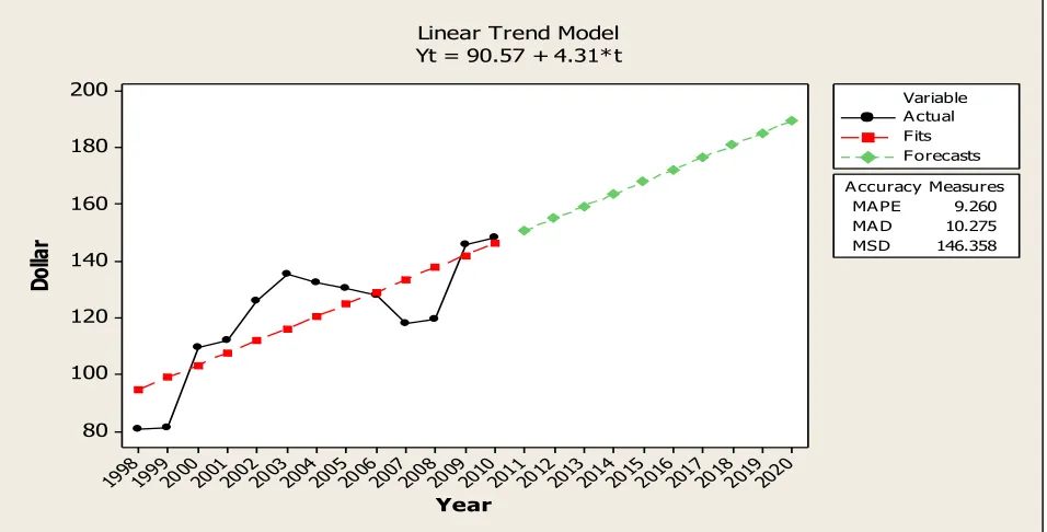
Linear Trend Model Yt = 90.57 + 4.31*t

Figure 2: Trend Analysis Plot for US Dollar (1998-2020)

2020 2019 2018 2017 2016 2015 2014 2013 2012 2011 2010 2009 2008 2007 2006 2005 2004 2003 2002 2001 2000 1999 1998

3000000

2500000

2000000

1500000

1000000

500000

0

Year

P

ou

nd

s

MAPE 4.44431E+01 MAD 2.06924E+05 MSD 6.88851E+10 Accuracy Measures

Actual Fits Forecasts Variable

Linear Trend Model Yt = -213484 + 126369*t

Figure 3: Trend Analysis Plot for Pounds Sterling (1998-2020)

Discussion

The figures 2 and 3 depict increase in the exchange rate of Naira to US Dollar and Pounds Sterling respectively. It is evident that the exchange rates of the currencies were on the high side over the years considered. Using linear model, the predicted values for both US Dollar and Pounds

(8)

184

Equation Obs Parms RMSE "R-sq" F P ---

Z1 13 2 13.15177 0.6399 19.54923 0.0010

Z1 13 2 27.5029 0.6392 19.48608 0.0010

---

| Coef. Std. Err. t P>|t| [95% Conf. Interval] ---+---

Z1 |

t | 4.310357 .9748739 4.42 0.001 2.164674 6.45604 _cons | 90.57119 7.737822 11.70 0.000 73.54036 107.602 ---+---

Z2 |

t | 8.999225 2.038651 4.41 0.001 4.512185 13.48627 _cons | 140.7688 16.18129 8.70 0.000 105.154 176.3836

Thus, the trend equations for future prediction of exchange rates of Us Dollar and Pounds sterling to Naira are

1

2

90.57119

4.310357 and

Z

140.7688

8.99925

Z

t









Respectively, since the models are significant at 1% (p-value of 0.0010), then, the (p-values of

Z

₁ and

Z

₂ in the nearest future can be computed from the Trend regressions. To determine future values of

Z

₁ and

Z

₂,

increase the time t from 13 (ie. year 2010) to desirable point, say 14 to 22. This implies predicting the values of US Dollar and Pounds exchange rate to Naira from 2011 to 2020. The result is as shown below

TABLE 5: PREDICTING THE VALUES OF US DOLLAR AND POUNDS EXCHANGE RATE TO NAIRA FROM 2011 TO 2020 Years T (time) US Dollar (

Z

₁) Pounds Sterling (

Z

₂)

2011 14 146.606 257.759

2012 15 150.916 266.758

2013 16 155.227 275.757

2014 17 159.537 284.756

2015 18 163.847 293.756

2016 19 168.158 302.755

2017 20 172.468 311.754

2018 21 176.778 320.753

2019 22 181.089 329.753

2020 23 185.399 338.752

The computed values gave the same result as shown in the figures 2 and 3, as the one US Dollar was projected to be the equivalent of 185.399naira in 2020 and 338naira for Pounds Sterling.

The models obtained from Existing method [5] are:

1 1 2

2 1 2

3 1 2

4 1 2

Model 1: Y

24141.1 6692.8

386.7 Model 2: Y

69236.9 12400.8

4459.8

Model 3: Y

162002.1 45664.2

53673.1

Model 4: Y

5647.6 600.7

384.2 Z

Z

 





 



 





 



(9)

185

Table 6: Projection for Oil Import, Non-Oil Import, Oil Export, Non-Oil Export from 2011 - 2020 using the Existing Method [5]

Years

US Dollar (

Z

₁)

Pounds Sterling

(

Z

₂) 1

Y

2

Y

3

Y

4

2011 146.606 257.759 856872 2898345 6978070 181449 2012 150.916 266.758 882222 2991932 7264257 187496 2013 155.227 275.757 907572 3085518 7550444 193543 2014 159.537 284.756 932923 3179105 7836632 199590 2015 163.847 293.756 958273 3272692 8122819 205636 2016 168.158 302.755 983623 3366278 8409006 211683 2017 172.468 311.754 1008974 3459865 8695194 217730 2018 176.778 320.753 1034324 3553451 8981381 223777 2019 181.089 329.753 1059674 3647038 9267568 229823 2020 185.399 338.752 1085025 3740625 9553755 235870

B. The models obtained from Existing Multivariate Bootstrap Algorithm [8] are:

The

Y s

_i

'

can be predicted using the values of

Z

₁ and

Z

₂ in the Table 5, and the projected values are shown in Table 7. Table 7: Projection for Oil Import, Non-Oil Import, Oil Export, Non-Oil Export from 2011 - 2020 using the Existing Multivariate

Bootstrap Algorithm [8]

Years

US Dollar (

Z

₁)

(

Z

₂) 1

Y

₂

Y

₃

Y

₄

2011 146.606 257.759 852102 2861427 6916816 179407 2012 150.916 266.758 877988 2955454 7204763 185533 2013 155.227 275.757 903875 3049480 7492710 191658 2014 159.537 284.756 929762 3143506 7780657 197784 2015 163.847 293.756 955648 3237532 8068604 203909 2016 168.158 302.755 981535 3331558 8356552 210035 2017 172.468 311.754 1007422 3425584 8644499 216160 2018 176.778 320.753 1033308 3519610 8932446 222286 2019 181.089 329.753 1059195 3613637 9220393 228411 2020 185.399 338.752 1085082 3707663 9508340 234537

C. The models obtained from the proposed Multivariate Jackknife Delete-5 Algorithm are:

 

1 1 2

2 1 2

3 1 2

4 1 2

ˆ

Model 1: Y

=

22038.3

5732.2

130.998 ˆ

Model 2: Y

62246.3

9960.02

5677.7

ˆ

Model 3: Y

151059

50960.96

56405.65

ˆ

Model 4: Y

5129.05

392.63

492.61

b

Z





 



 





(10)

186 5

5

( )

1 1 2

( )

2 1 2

( )

3 1 2

( )

4 1 2

ˆ

Model 1: Y

=

23906.6 6583.5

386.7 ˆ

Model 2 : Y

68525.3 12175.6

4569.6

ˆ

Model 3 : Y

160841 46193

53948.8

ˆ

Model 4 : Y

5593 23906.6

6583.5

d

d d d

J

Z







 



 





 





The

Y s

_i

'

can be predicted using the values of

Z

₁ and

Z

₂in Table 5, the projected values are shown in Table 8.

TABLE 8: Projection for Oil Import, Non-Oil Import, Oil Export, Non-Oil Export from 2011 - 2020 using the Proposed Multivariate Jackknife Delete-5 Method Algorithm

Years

US Dollar (

Z

₁)

(

Z

₂) 1

Y

2

Y

3

Y

4

2011 146.606 257.759 841598 2894343 6973028 -1813485 2012 150.916 266.758 866495 2987947 7259426 -1857285 2013 155.227 275.757 891392 3081551 7545824 -1901085 2014 159.537 284.756 916289 3175155 7832222 -1944884 2015 163.847 293.756 941187 3268759 8118620 -1988684 2016 168.158 302.755 966084 3362363 8405018 -2032483 2017 172.468 311.754 990981 3455967 8691416 -2076283 2018 176.778 320.753 1015878 3549571 8977814 -2120082 2019 181.089 329.753 1040775 3643175 9264212 -2163882 2020 185.399 338.752 1065673 3736779 9550610 -2207682

The negative sign of the values in the column 7 (Y4) is an indication of reduction in the values of non-oil export from the initial

state as a result of depreciation of Nigeria currency. This implies the possibility of great reduction of non-oil export value in some years to come.

3.0 Findings and Conclusion

It is evidently an increase of exchange rate of US Dollar and Pounds Sterling affects Oil import, Oil export, Non-oil import and Non-oil export (Foreign Trade) negatively which could be harmful to the nation’s economy. The importance of Foreign Trade to any nation is to increase in the GDP of that Nation, but the reduction in elements of Foreign Trade, definitely, will lead to reduction in the GDP of such nation. Therefore, stability of Foreign exchange rates of US Dollar and Pounds Sterling to Naira should be sustained to a rate that will burst the Nation’s economy.

References:

[1]. Adebiyi, M.A., Adenuga, A.O., Abeng, M.O. and Omanukwue, P.N. (2010). Oil Price Shocks, Exchange Rate and Stock Market Behaviour: Empirical Evidence from Nigeria, working paper, presented in the research department of Central Bank of Nigeria.

[2]. Central Bank of Nigeria Statistical Bulletin, Central Bank of Nigeria, Gariki Abuja, Nigeria, 2011.

[3]. Efron, B., The Jackknife, the Bootstrap and other Resampling Plans, CBNS-NSF Regional Conference Series in Applied Mathematics, 1982, 38, 29-35.

[4]. Efron, B., Second Thought on Bootstrapping. Statistical Science, 2003, 18(2), 135-140.

[5].Johnson,R. A. and Wichern, D.W., Applied Multivariate Statistical Analysis.Third Edition, Prentice Hall, Englewood Cliffs, New Jersey ,1992, 314-316.

[6]. Maksui et al, Multivariate Functional Analysis, Journal of Productive Analysis, 2008, 29, 27

[7]. Obiora-Ilouno,H.O.andMbegbu,J.I., Bootstrap Algorithm for the Estimation of Logistic Regression Parameters. Journal of Nigerian Statistical Association (NSA), Nigeria, 2012, 24, 10-19

(11)

187

Foreign Trade on Foreign Exchange Rates of Naira Using Bootstrap Approach, Accepted paper in

"Studies in Mathematical Sciences", 2013, Volume 6, Number 3.(To appear in 31st May 2013).

APPENDIX

A. The data obtained from Central Bank of Nigeria Bulletin 2010 edition on exchange of US Dollar and Pounds to Nigeria naira currency and Nigeria foreign trade from 1960-2010 and shown in the table below.

YEARS

US DOLLAR POUNDS

OIL (IMPORT)

NON-OIL (IMPORT)

OIL (EXPORT)

NON-OIL (EXPORT)

1960 0.7143 2 26.952 404.83 8.816 330.612

1961 0.7143 2 31.668 413.37 23.09 324.166

1962 0.7143 2 32.966 373.468 34.42 302.652

1963 0.7143 2 37.258 377.916 40.354 338.306

1964 0.7143 2 46.398 461.028 64.112 365.19

1965 0.7143 2 47.876 502.186 136.194 400.58

1966 0.7143 2 22.042 490.666 183.94 384.228

1967 0.7143 2 23.228 417.872 144.772 340.866

1968 0.7143 2 39.642 345.76 73.998 348.12

1969 0.7143 2 42.766 454.616 261.93 374.062

1970 0.7143 1.7114 38.702 717.718 509.622 376.046

1971 0.6955 1.7156 50.4 1028.5 953 340.4

1972 0.6579 1.6289 45.2 944.9 1176.2 258

1973 0.6579 1.6289 41 1183.8 1893.5 384.9

1974 0.6299 1.4795 52.4 1684.9 5365.7 429.1

1975 0.6159 1.3618 118 3603.5 4563.1 362.4

1976 0.6265 1.1317 95 5053.5 6321.6 429.5

1977 0.6466 1.1671 102.2 6991.5 7072.8 557.9

1978 0.606 1.2238 110 8101.7 5401.6 662.8

1979 0.5957 1.2628 230 7242.5 10166.8 670

1980 0.5464 1.2647 227.4 8868.2 13632.3 554.4 1981 0.61 1.2495 119.8 12719.8 10680.5 342.8

1982 0.6729 1.1734 225.5 10545 8003.2 203.2

1983 0.7241 1.1216 171.6 8732.1 7201.2 301.3 1984 0.7649 1.0765 282.4 6895.9 8840.6 247.4 1985 0.8938 1.1999 51.8 7010.8 11223.7 497.1 1986 2.0206 2.5554 913.9 5069.7 8368.5 552.1 1987 4.0179 6.5929 3170.1 14691.6 28208.6 2152 1988 4.5367 8.0895 3803.1 17642.6 28435.4 2757.4 1989 7.3916 12.0695 4671.6 26188.6 55016.8 2954.4 1990 8.0378 16.2419 6073.1 39644.8 106626.5 3259.6 1991 9.9095 17.4955 7772.2 81716 116858.1 4677.3 1992 17.2984 27.8684 19561.5 123589.7 201383.9 4227.8 1993 22.0511 33.2522 41136.1 124493.3 213778.8 4991.3 1994 21.8861 33.4252 42349.6 120439.2 200710.2 5349 1995 21.8861 34.524 155825.9 599301.8 927565.3 23096.1 1996 21.8861 34.7698 162178.7 400447.9 1286215.9 23327.5 1997 21.886 36.2166 166902.5 678814.1 1212499.4 29163.3 1998 81.0228 128.1561 175854.2 661564.5 717786.5 34070.2 1999 81.2528 126.4165 211661.8 650853.9 1169476.9 19492.9 2000 109.55 163.0323 220817.69 764204.7 1920900.4 24822.9 2001 112.4864 161.7534 237106.83 1121073.5 1839945.25 28008.6 2002 126.4 203.7442 361710 1150985.33 1649445.828 94731.85 2003 135.40 234.4 398922.31 1681312.96 2993109.95 94776.44 2004 132.67 249.9925 318114.72 1668930.55 4489472.19 113309.4 2005 130.4 221.2385 797298.94 2003557.39 7140578.92 105955.9 2006 128.27 249.3899 710683 2397836.32 7191085.64 133595 2007 117.968 234.0205 768226.84 3143725.79 8110500.38 199257.9 2008 119.7925 216.4808 1386729.93 3803072.68 9913651.13 247839 2009 146 231.6438 1063544.18 4038990.2 8067233 289152.6 2010 148.455 228.6553 2073579.03 5931795.19 10639417.37 396377.2

(12)

188

B. IMPLEMENTATION OF MULTIVARIATE DELETE-d ALGORITHM FOR ESTIMATION OF THE PARAMETERS OF MULTIVARIATE LINEAR MODEL

#part 1:To read data

data=read.table("data(hap).txt", header=T, sep="")

#Part 2

#Run this to get the original estimates

data=data.frame(data)

reg=lm(cbind(y1, y2, y3, y4) ~ x1+x2,data=data)

reg

summary(reg)

#Delete d jacknife algorithm begins here

#d=no of rows to be deleted

#p=no of cols in the data

#data is the data matrix with the first p1 columns

#for the dept vars and the remaining p-p1 cols for the indpt vars

jack.a=function(data,p1,d)

{

p=ncol(data)

n=nrow(data)

u=combn(n,d) #Assign the matrix of all possible combinations to u

output=matrix(0,ncol=p1*(p-p1)+p1,nrow=ncol(u))

y=data[,1:p1] #the responses

x=data[,(p1+1):p] #the covariates

for (i in 1:(ncol(u)))

{

dd=c(u[,i])

yn=y[-dd,] #delete d rows of the independent var

xn=x[-dd,] #delete d rows of the dependent var

reg=lm(formula=yn~xn)

coef=coef(reg)

output[i,]=c(as.vector(coef))

(13)

189

output

}

#Use this part to run

data=data.matrix(data)

run=jack.a(data,2,5)

est=c(mean(run[,1],na.rm=TRUE),mean(run[,2],na.rm=TRUE),mean(run[,3],na.rm=TRUE),mean(run[,4],na.rm=TRUE),mean(run [,5],na.rm=TRUE),mean(run[,6],na.rm=TRUE),mean(run[,7],na.rm=TRUE),mean(run[,8],na.rm=TRUE),mean(run[,9],na.rm=TRU E),mean(run[,10],na.rm=TRUE))

> est1=matrix(est,3,4)

> rownames(est1)=c("Intercept","x1","x2")

> colnames(est1)=c("y1","y2","y3","y4")