Interfacial Wave Dynamics Of Core-Annular Flow Of Two Fluids

(1)

University of Pennsylvania

ScholarlyCommons

Publicly Accessible Penn Dissertations

2018

Interfacial Wave Dynamics Of Core-Annular Flow

Of Two Fluids

Mohammed Asaduzzaman

University of Pennsylvania, [email protected]

Follow this and additional works at:https://repository.upenn.edu/edissertations

Part of theMechanical Engineering Commons

This paper is posted at ScholarlyCommons.https://repository.upenn.edu/edissertations/2798 For more information, please [email protected].

Recommended Citation

Asaduzzaman, Mohammed, "Interfacial Wave Dynamics Of Core-Annular Flow Of Two Fluids" (2018).Publicly Accessible Penn Dissertations. 2798.

(2)

Interfacial Wave Dynamics Of Core-Annular Flow Of Two Fluids

Abstract

In core-annular flow of two different fluids, for a set of suitable flow conditions, various shapes of saturated waves such as bamboo, snake and corkscrew waves are observed. Some of the dominant parameters such as thickness ratio of the fluid, Reynolds number, viscosity ratio, density ratio, interfacial surface tension, and the direction of gravitational forces determine the final shape of the saturated wave and their ultimate stability in a nonlinear regime.

When the flow rate ratio is high, it is sometimes difficult to determine the differences between the final shape of the waves for up-flow and down-flow. For some combinations of thickness ratio, viscosity ratio, density ratio, Reynolds number and surface tension, waves tend to break and bubbles start to form. Interfacial surface tensions between these two fluids play a very important role in stabilizing the waves from breaking.

In this study, new sets of waves were discovered for core-annular flow, which modulate at certain flow parameter ranges. The critical parameter ranges are identified where the waves shift from saturated bamboo waves and bifurcate into modulated bamboo waves. A thorough analysis is performed for the first time to depict the windows of these critical parameters at which this transition takes place. A bifurcation diagram is constructed to capture the regime. A detailed wave shape analysis is performed to characterize these wave shapes and their periods of oscillation.

Due to challenges associated with large computational domain and enormous computational power requires to resolve the interfacial instability, a three-dimensional true non-axisymmetric model was never studied before. For the first time, effort is being undertaken to construct a viable 3-D Core-annular flow. A general purpose computational fluid dynamics package ANSYS Fluent is used for this analysis. Three dimensional models for both up-flow and down-flow were constructed and a novel explanation is presented to distinguish between the Bamboo waves, Cork-Screw waves, and Snake waves. The sensitivity of down-flow on initial conditions was also verified with 3-D models on some parameter space from selected publication.

Degree Type

Dissertation

Degree Name

Doctor of Philosophy (PhD)

Graduate Group

Mechanical Engineering & Applied Mechanics

First Advisor

Howard H. Hu

Keywords

Bamboo waves, Core-annular Flow, Corkscrew Wave, Interfacial Instability, Snake Waves, Wave Dynamics

(3)

Subject Categories

Mechanical Engineering

(4)

i

INTERFACIAL WAVE DYNAMICS OF CORE-ANNULAR

FLOW OF TWO FLUIDS

A DISSERTATION in

Mechanical Engineering and Applied Mechanics

Presented to the Faculties of the University of Pennsylvania in

Partial Fulfillment of the Requirements for the Degree of Doctor of Philosophy

2018

Supervisor of Dissertation

_________________________________________ Howard H. Hu

Professor of Mechanical Engineering and Applied Mechanics

Graduate Group Chairperson

_______________________________________

Kevin Turner, Professor of Mechanical Engineering and Applied Mechanics

Dissertation Committee

(5)

ii

INTERFACIAL WAVE DYNAMICS OF CORE-ANNULAR

FLOW OF TWO FLUIDS

©COPYRIGHT

2018

(6)

iii

(7)

iv

ACKNOWLEDGEMENT

First, I would like to express immense gratitude to my advisor Dr. Howard Hu. Without his support, guidance and patience, I would not have been able to continue my journey. I started to pursue Ph.D. as a part-time student while working full-time. It was extremely challenging for me to balance both school and work. I am fortunate to have encountered the best and brightest minds who have helped me tremendously with my aspiration to obtain my doctorate degree.

I came across various obstacles during the course of my studies. With the guidance and advice of Dr. Hu, I found myself with a new sense of spirit. I also received significant one-on-one time from Dr. Hu to learn and clarify my questions about many subject matters. I am also grateful to Dr. Hu to provide me with an opportunity to serve as a teaching assistant on Numerical Methods and Finite Element Analysis class. This experience opened my mind in many ways including helping me to understand how to interact with students and learn the teaching methodology.

(8)

v

Moreover, I would also like to thank some of the members of Dr. Bau’s and Dr. Hu’s research lab for valuable discussions during my time at University of Pennsylvania. Special thanks to Dr. Tong Gao and Dr. Barukiha Shapinko.

I would also like to thank all of the faculty members of University of Pennsylvania with whom I have taken classes and learn valuable lessons. I would also like to convey my sincerest appreciation to Maryeileen Branford and Peter Litt who helped me a great deal in supporting my graduate studies.

I must recognize Ansys ™ technical support team with whom I shared a significant amount of time. Special thanks to Dr. Yi Dai with whom, I discussed about the sensitivity of the Fluent™ explicit formulation and sharp interface techniques to improve the quality

of our modeling effort. Assistance provided by Dr. Anuraddha Mukhopadhyey of Ansys™ over the years, is greatly appreciated.

I am also indebted to DuPont Engineering Research and Technology for financially supporting my studies. Special thanks go to my former managers Arche Bice, Glenn Hake and my former colleagues Dr. Kevin Allred, Dr. Minye Liu and Dr. John Young for their inspiration during my seventeen-year career with DuPont.

(9)

vi

(10)

vii

ABSTRACT

INTERFACIAL WAVE DYNAMICS OF CORE-ANNULAR FLOW OF

TWO FLUIDS

Howard H. Hu

In core-annular flow of two different fluids, for a set of suitable flow conditions, various shapes of saturated waves such as bamboo, snake and corkscrew waves are observed. Some of the dominant parameters such as thickness ratio of the fluid, Reynolds number, viscosity ratio, density ratio, interfacial surface tension, and the direction of gravitational forces determine the final shape of the saturated wave and their ultimate stability in a nonlinear regime.

When the flow rate ratio is high, it is sometimes difficult to determine the differences between the final shape of the waves for up-flow and down-flow. For some combinations of thickness ratio, viscosity ratio, density ratio, Reynolds number and surface tension, waves tend to break and bubbles start to form. Interfacial surface tensions between these two fluids play a very important role in stabilizing the waves from breaking.

(11)

viii

waves shift from saturated bamboo waves and bifurcate into modulated bamboo waves. A thorough analysis is performed for the first time to depict the windows of these critical parameters at which this transition takes place. A bifurcation diagram is constructed to capture the regime. A detailed wave shape analysis is performed to characterize these wave shapes and their periods of oscillation.

(12)

ix

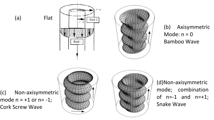
Figure 1: Schematic of possible Core Annular Flow Wave Shapes: (a) Flat Interface (b) Axisymmetric Bamboo Wave (c) Non-Axisymmetric Cork Screw Wave (d) Non-Axisymmetric Snake Wave ... 2 Figure 2: (a) Bamboo waves observed in up flows of motor oil and water. The oil has a viscosity of 13.32 poise and a density of 0.881 g/cm^3 at room temperature T = 22 °C. The volume flow rates are Qo = 0.11332 gpm, Qw = 0.05284 gpm (from BCJ 1990) (b) Corkscrew waves are observed in down-flows of motor oil and water. The oil has a viscosity of 13.32 poise and a density of 0.881 g/cm3_{at room temperature T = 22° C and volume flow rate Qo = 0.8212 gpm,} Qw = 0.05284 gpm ... 3 Figure 3: Schematic of core-annular flow. ... 22 Figure 4: Interface calculation and interpolation scheme of ANSYS Fluent (Fluent Theory Manual v18.2, page 561). (a) Actual interface shape (b) Interface shape represented by the geometric reconstruction (piecewise-linear) scheme. ... 42 Figure 5: Plot of growth rate vs. wave number for the benchmark case. ... 48 Figure 6: Velocity profile at the core and annulus for the basic flow in dimensional form.

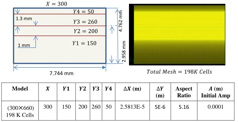
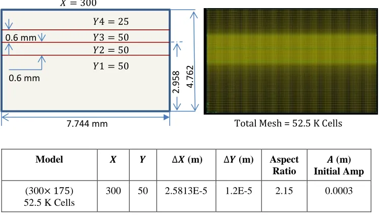
... 49 Figure 7: Schematic diagram of 2-D axisymmetric problem set-up and boundary conditions for fixed wall configuration. ... 50 Figure 8: Schematic diagram of problem set-up and boundary conditions with moving frame of reference. ... 51 Figure 9: Mesh layout for growth rate calculation. Total computational cell size is (300×560) =198K. ... 52 Figure 10: Mesh layout for the benchmark case. Total computation mesh size is ~ 52K.

(17)

xiv

(18)

xv

Figure 30: Wave shape at every 0.05 seconds time interface for surface tension parameter 𝐽 = 3𝐽𝑏. Waves were shifted in the horizontal direction to match with reference wave at time t. ... 83 Figure 31: Comparison of wave shapes for saturated bamboo wave regime (in scale) at different surface tension parameters. ... 84 Figure 32: Comparison of wave shapes in non-dimensional form at saturated bamboo wave regime at different surface tension parameters. ... 84 Figure 33: Amplitude vs surface tension parameters for saturated bamboo wave regime. Curve fit of the amplitudes with respect to surface tension shows nonlinear relationship. ... 85 Figure 34:Saturated and modulated bamboo wave regime with variable amplitudes. .... 86 Figure 35: Base Case Amplitude Vs. Time for surface tension parameters 𝐽 = 𝐽𝑏 =

0.063354. ... 87 Figure 36: Amplitude Vs. Time for the saturated wave for the benchmark case with surface tension parameter 𝐽 = 𝐽𝑏. ... 88 Figure 37: Wave shape at three Peak to Peak locations for benchmark case of surface tension 𝐽 = 𝐽𝑏. ... 89 Figure 38: Amplitude vs. Time curve for the benchmark case of surface tension 𝐽 = 𝐽𝑏.

Three vertical lines are showing the Valley to Valley amplitude as a function of time. ... 89 Figure 39: Valley to Valley three waves are identical in shape for benchmark case of surface tension 𝐽 = 𝐽𝑏. Waves are shifted only in X- direction. ... 90 Figure 40: Comparison between the peak and valley wave shape for 𝐽 = 𝐽𝑏. ... 91 Figure 41: Temporal location of waves and its amplitude at every 0.003 seconds of simulation time. Covering the waves between peak and valley. Vertical lines are the identification of temporal location and corresponding wave amplitudes. ... 91 Figure 42: Wave shape at every 0.003 seconds time interval. (𝐽 = 1 × 𝐽𝑏 = 0.063, 𝑎 =

(19)

xvi

Figure 44: Non-dimensional wave shape at every 0.003 seconds time interval capturing the wave shape from peak to valley. Wave shapes were shifted in the horizontal direction to match with the maximum height of the first wave at time t. ... 93 Figure 45: Temporal location of Peak to Peak wave for the surface tension parameter 𝐽 =

2𝐽𝑏 = 0.127. ... 95 Figure 46: Solid lines are Peak to Peak wave shapes for surface tension parameter 𝐽 = 2𝐽𝑏.

Dotted lines are the shifted waves and they perfectly coincide with each other. Peak to Peak waves repeat itself after every 0.034 seconds. ... 95 Figure 47: Temporal location of the Valley to Valley waves for the surface tension parameter 𝐽 = 2𝐽𝑏 = 0.127. ... 96 Figure 48: Solid lines are Valley to Valley wave shape for surface tension parameter 𝐽 =

(20)

xvii

Figure 59: (a) Evolution of the wave shape at different times for surface tension parameter 𝐽 = (1/16)𝐽𝑏. (b) Wave shape with enlarged view close to the interface. 106

Figure 60: Wave shape close to wave breaking for surface tension parameter 𝐽 = (1/16)𝐽𝑏. ... 106 Figure 61: Wave Speed as a function of surface tension. ... 107 Figure 62: Hold-up ratio at different surface tension parameters. ... 109 Figure 63: Growth rate versus wave number at different surface tension parameters at fixed Reynolds number of ℝ =3.737 ... 111 Figure 64: Growth Rate Vs. Wave Number for various Reynolds number with fixed flow parameters of 𝐽 = 𝐽𝑏 = 0.063354,𝑎 = 1.61,𝑚 = 0.00166389,𝜁 = 1.1.114 Figure 65: Growth rate vs. Wave number at various Reynolds numbers. ℝ = 7 and ℝ =

10 shows maximum growth at lower wave number. ... 115 Figure 66: Wave Number corresponds to maximum growth rate as a function of Reynolds number. For fix flow parameters of 𝐽 = 𝐽𝑏 = 0.063,𝑎 = 1.61,𝑚 = 0.00166, 𝜁 = 1.1. ... 116 Figure 67: Wave amplitudes at different ranges of Reynolds numbers for a fixed surface tension parameter, 𝐽 = 𝐽𝑏 = 0.0633 and other fixed parameters 𝑎 = 1.61, 𝑚 = 0.00166,𝜁 = 1.1. ... 119 Figure 68: Amplitude of saturated wave for Reynolds number ℝ = 2. Three vertical lines are showing the location of the Peak to Peak wave amplitude and the corresponding simulation time. ... 120 Figure 69: Comparison of Peak to Peak saturated waves for Reynolds number ℝ = 2. 120 Figure 70: Amplitude of saturated wave for Reynolds number ℝ = 2. Three vertical lines are showing the location of the Valley to Valley wave amplitudes and the corresponding simulation time. ... 121 Figure 71: Comparison of Valley to Valley saturated waves for Reynolds number ℝ = 2

(21)

xviii

(22)

xix

Figure 87: Saturated bamboo wave shape (actual dimension) at different Reynolds number for a fixed surface tension parameter of 𝐽 = 𝐽𝑏 = 0.0633. and other fixed parameters (𝑎 = 1.61,𝑚 = 0.0016,𝜁 = 1.1). ... 132 Figure 88: Peak to Peak wave shapes in non-dimensional form for saturated bamboo wave regime at different Reynolds numbers. ... 133 Figure 89: Bifurcation diagram of wave amplitude at different Reynolds numbers for a fixed surface tension parameter of 𝐽 = 𝐽𝑏 = 0.0633 and other fixed parameters (𝑎 = 1.61,𝑚 = 0.00166,𝜁 = 1.1). ... 134 Figure 90: Phase diagram describing the stability of the flow regime for the range of Reynolds numbers and surface tension parameters. ... 136 Figure 91: Wave speed (non-dimensional) at different Reynolds numbers for a fixed surface tension parameter of 𝐽 = 𝐽𝑏 = 0.063. and other fixed parameters (𝑎 = 1.61,𝑚 = 0.00166,𝜁 = 1.1). ... 137 Figure 92: Hold-up ratio at different Reynolds numbers for fixed flow parameters of 𝐽 =

(23)

xx

Figure 102: Wave shape from 3-D simulation. Interface waves of three consecutive domains (three wave lengths) show the wave shape for the benchmark flow parameters. They constitute the shape of a bamboo stem. ... 149 Figure 103: Volumetric fraction of the saturated wave. Blue represents oil, red represents water and green represents three-dimensional interfacial surface. A view at z=0 also shows the maximum and minimum interfacial wave height. ... 150 Figure 104: Comparison between the amplitudes of waves of 2-D axisymmetric model and 3-D model. ... 151 Figure 105: Oscillation of the wave amplitudes of 3-D model. Vertical lines showing Peak to Peak wave locations. ... 153 Figure 106: Comparison of Peak to Peak waves of the 3-D model. Waves are shifted in the x-direction to match with initial peak wave at time t. ... 153 Figure 107: Oscillation of the wave amplitudes of 3-D model. Vertical line showing Valley to Valley wave location. ... 154 Figure 108: Comparison of Valley to Valley waves of the 3-D model. Waves are shifted in the x-direction to match with initial valley wave at time t. ... 154 Figure 109: Comparison of Peak to Peak and Valley to Valley wave shapes. Valley wave is shifted in x-direction to match the maximum wave height of the Peak wave. ... 155 Figure 110: Wave shape comparison of published 2-D results, 2-D axisymmetric Fluent™ model and 3-D Fluent™ model. ... 156 Figure 111: Comparison of hold-up ratio in non-dimensional time scale at saturation between 2-D axisymmetric and 3-D models of ANSYS Fluent results vs. Published 2-D results. ... 158 Figure 112: Geometric representation of various models of interfacial waves. ... 160 Figure 113: Growth rate versus wave number for axisymmetric and asymmetric disturbances. The flow conditions are taken the same as experiment No. 6 in Bai et al. (1992) [𝑎 = 1.7, 𝑚 = 0.00166, 𝜁 = 1.1, 𝐽 = 0.063354, 𝐾 = −0.5427 and 𝛼 = 0.531]. ... 161 Figure 114: Pattern selection results for (𝑎 = 1.7, 𝑚 = 0.00166,𝜁 = 1.1, 𝐽 = 0.063354,

(24)

xxi

Reynolds number R1 in which corkscrews (C) are preferred, snakes (S) are preferred, or neither (N). ... 163 Figure 115: Problem set-up and mesh configuration for ℝ= 1.2. ... 165 Figure 116:A typical trajectories of the centrodial coordinates of core fluid of an arbitary cross-section over time for a corkscrew wave. The movment of the centroidal coordinate follows a circular path. ... 167 Figure 117: A typical trajectories of the centrodial coordinates of core fluid of an arbitary cross-section over time for a snake wave. The movment of the centroidal coordinate follows a strait line. ... 167 Figure 118: Evolution of 3-D non-axisymmetric corkscrew wave over time [𝑎 = 1.7,𝑚 =

0.00166,𝜁 = 1.1, 𝐽 = 0.063,𝐾 = −0.5427, 𝛼 = 0.531 and ℝ=1.2]. ... 168 Figure 119: Slice of core-annular section at the center X-Y plane of the pipe. [𝑎 = 1.7,𝑚 =

0.00166,𝜁 = 1.1, 𝐽 = 0.063,𝐾 = −0.5427, 𝛼 = 0.531 and ℝ=1.2]. ... 169 Figure 120: Interface wave shape at two different times obtained from top X-Y plane section for the following flow parameters 𝑎 = 1.7,𝑚 = 0.00166,𝜁 = 1.1, 𝐽 = 0.063, 𝐾 = −0.5427, 𝛼 = 0.531 and ℝ=1.2. ... 169 Figure 121: Nonaxisymmetric corkscrew wave shape taken at interface at the center cross section plane. For better visualization, wave shapes are drawn for two wave lengths. [𝑎 = 1.7, 𝑚 = 0.00166, 𝜁 = 1.1, 𝐽 = 0.063, 𝐾 = −0.5427, 𝛼 = 0.531 and ℝ=1.2]. ... 170 Figure 122: Evolution of corkscrew wave. Movement of the centroidal coordinates over time [𝑎 = 1.7, 𝑚 = 0.00166, 𝜁 = 1.1, 𝐽 = 0.063,𝐾 = −0.5427, 𝛼 = 0.531 and ℝ=1.2]. (a) At time = 3.08 seconds (b) time = 3.035 seconds (c) time = 3.08 seconds and (d) time = 3.1475 seconds. ... 173 Figure 123:Movement of the coordinate 𝑌𝑚 and 𝑍𝑚 over time [𝑎 = 1.7,𝑚 = 0.00166,

𝜁 = 1.1, 𝐽 = 0.063,𝐾 = −0.5427, 𝛼 = 0.531 and ℝ=1.2]. ... 174 Figure 124: Movement of 𝑌𝑚 vs. time and 𝑍𝑚 Vs. time [𝑎 = 1.7, 𝑚 = 0.00166, 𝜁 =

(25)

xxii

Figure 127: Evolution of the interface waves at earlier simulation time. Plots are showing the change in centroidal coordinate of the core fluid over time. Movement of the centroidal coordinate 𝑍𝑚 and 𝑌𝑚 over time is in a straight line. [𝑎 = 1.7, 𝑚 = 0.00166, 𝜁 = 1.1, 𝐽 = 0.063, 𝐾 = −0.5427, 𝛼 = 0.531 and ℝ=1.2]. ... 178 Figure 128: Evolution of interface waves at longer simulation time. 𝑍𝑚 vs. 𝑌𝑚 plot is the movement of centroidal coordinate of the core fluid at an arbitrary location. This plots shows a shift from line to a circular trajectory. 𝑌𝑚 vs. Time and 𝑍𝑚 vs. Time curve show the movement of the centroidal coordinate over time. [𝑎 = 1.7, 𝑚 = 0.00166, 𝜁 = 1.1, 𝐽 = 0.063, 𝐾 = −0.5427, 𝛼 = 0.531 and ℝ=1.2]. ... 179 Figure 129: Evolution of the interfacial wave shape for Case II (ℝ = 0.9). The centroidal coordinates (𝑍𝑚 and 𝑌𝑚) of the core fluid trajectories shows a circular path. Therefore, the interfacial wave travels in both azimuthal and axial direction and the waves are corkscrew waves. [𝑎 = 1.7, 𝑚 = 0.00166, 𝜁 = 1.1, 𝐽 = 0.063354,𝐾 = −0.5427 and 𝛼 = 0.531 and ℝ = 0.9] ... 182 Figure 130: Trajectories of the centroidal coordinates (𝑍𝑚 vs. 𝑌𝑚) of the core fluid at an arbitrary cross section over time for case II. [𝑎 = 1.7, 𝑚 = 0.00166, 𝜁 = 1.1, 𝐽 = 0.063354,𝐾 = −0.5427 and 𝛼 = 0.531 and ℝ = 0.9]. ... 183 Figure 131: Trajectories of the centroidal coordinates (𝑌𝑚 vs. time and 𝑍𝑚 vs. time) of the core fluid at an arbitrary cross section over time for case II. [𝑎 = 1.7, 𝑚 = 0.00166, 𝜁 = 1.1, 𝐽 = 0.063354, 𝐾 = −0.5427 and 𝛼 = 0.531 and ℝ = 0.9]. ... 184 Figure 132: Trajectories of the centroidal coordinates (𝑍𝑚 and 𝑌𝑚) of the core fluid at an arbitrary cross section over time for case II in 3-D plot[𝑎 = 1.7,𝑚 = 0.00166, 𝜁 = 1.1, 𝐽 = 0.063354,𝐾 = −0.5427 and 𝛼 = 0.531 and ℝ = 0.9]. ... 184 Figure 133: Few representative wave shapes at different simulation times. [𝑎 = 1.7,𝑚 =

(26)

xxiii

Figure 137: Wave shapes at two different times obtained from top X-Y plane section. Only the top portion of the waves are shown. [𝑎 = 1.7,𝑚 = 0.00166,𝜁 = 1.1, 𝐽 = 0.063354,𝐾 = −0.5427 and 𝛼 = 0.531 and ℝ = 0.9]. ... 188 Figure 138: Non-axisymmetric corkscrew wave shapes taken at interface at the center cross section (X-Y) plane. Only the top portion of the waves are shown. For better visualization, wave shapes are drawn for two wave lengths. [𝑎 = 1.7, 𝑚 = 0.00166, 𝜁 = 1.1, 𝐽 = 0.063354, 𝐾 = −0.5427 and 𝛼 = 0.531 and ℝ = 0.9]. ... 188 Figure 139: Evolution of the wave shapes for Case III (ℝ= 0.525 ). [𝑎 = 1.7,𝑚 = 0.00166,

𝜁 = 1.1, 𝐽 = 0.063354,𝐾 = −0.5427 and 𝛼 = 0.531]... 190 Figure 140: Movement of the centroidal coordinate (𝑍𝑚 vs. 𝑌𝑚 ) of the core fluid at an arbitrary location over time. ... 191 Figure 141: Movement of the centroidal coordinates (𝑍𝑚 vs. time and 𝑌𝑚vs. time) of the core fluid at an arbitrary location over time. ... 191 Figure 142: movement of the centroidal coordinates in 3-D plot with respect to time.

Movement of the centroidal coordinate (𝑍𝑚, 𝑌𝑚) over time confirms that the wave shape is indeed a snake wave. ... 192 Figure 143: Figure: Re 0.525: Case III, combination of bamboo wave and weak snake wave. Interface wave shape (green). ... 193 Figure 144: Re 0.525: Case III, combination of bamboo wave and weak snake wave. Interface wave shape (green). ... 194 Figure 145: Comparison of the Top and Bottom wave shapes at simulation time 3.48 sec.

Bottom wave height is adjusted to match with Top wave height. ... 195 Figure 146: Comparison of the Top and Bottom wave shapes at simulation time 3.7 sec.

(27)

xxiv

0.00166, 𝜁 = 1.1, 𝐽 = 0.063354, 𝐾 = −0.5427 and 𝛼 = 0.531, ℝ = 0.525 ]. ... 198 Figure 150: Change in wave speed as a function of Reynolds number. ... 198 Figure 152: Peak to Peak wave shape comparison for the surface tension parameter 𝐽 =

(1/2)𝐽𝑏 = 0.03167. Solid lines are the waves and dotted lines are shifted waves to match the initial wave at time t. They perfectly overlap. ... 205 Figure 153: Valley to Valley wave shape comparison for the surface tension parameter 𝐽 =

(1/2)𝐽𝑏 = 0.03167. Solid lines are the waves and dotted lines are shifted waves to match the initial wave at time t. They perfectly overlap. ... 206 Figure 154: Peak to Peak and Valley to Valley wave shape comparison for surface tension parameter 𝐽 = (1/2)𝐽𝑏 = 0.03167. ... 206 Figure 155: Peak to Peak wave shape comparison for 𝐽 = (1/4)𝐽𝑏. ... 207 Figure 156: Valley to Valley wave shape comparison for 𝐽 = (1/4)𝐽𝑏... 208 Figure 157: Peak to Peak and Valley to Valley wave shape comparison for 𝐽 = (1/4)𝐽𝑏.

... 208 Figure 158: Amplitude Vs. Time. Three lines showing the temporal location of the waves at every 0.005sec from starting time t. ... 209 Figure 159: Wave shape at every 0.005 seconds from initial starting starting time t. .... 209 Figure 160: Amplitude Vs. time curve. Three lines showing the temporal location of the waves at every 0.005seconds interval. ... 210 Figure 161: Wave shape at very 0.005 seconds for the surface tension parameter of 𝐽 =

(28)

xxv

(29)

1

CHAPTER 1 : Introduction

1.1 Background and motivation

When two immiscible fluids are forced to flow through a confined space simultaneously there is a natural tendency for the fluid with lower viscosity to migrate in to the region of high shear. This natural tendency opens up lots of interesting technological applications where one fluid is used to lubricate another. One such application is transportation of crude viscous oil with another fluid with lower viscosity. The pumping energy required to push the viscous oil from its origin to a secondary destination is enormous, as it has to overcome the shear stress generated at the wall of the pipe. This lubricated mechanism of oil at the core and water at the annulus is called core-annular flow (CAF).

(30)

2

Figure 1: Schematic of possible Core Annular Flow Wave Shapes: (a) Flat Interface (b) Axisymmetric Bamboo Wave (c) Non-Axisymmetric Cork Screw Wave (d) Non-Axisymmetric Snake Wave

In Figure 1(b), wavy interface bamboo wave is illustrated. The bamboo waves are axisymmetric in nature and has pointed peak and wider trough and they are usually symmetric to peak. In Figure 1(c) and Figure 1(d), typical corkscrew and snake wave shapes are shown. Both corkscrew and snake waves are non-axisymmetric waves however corkscrew wave travels in both axial direction as well as azimuthal direction on the other hand snake waves only travel in axial direction.

Bai, Chen, and Joseph D. (1992) published their experimental work of the core-annular flow for a pipe and they observed both bamboo waves and corkscrew waves. A typical shape of bamboo wave is shown in Figure 2 (a) and a representative diagram of corkscrew wave is presented in Figure 2 (b).

(d)Non-axisymmetric mode; combination of n=-1 and n=+1; Snake Wave

(a) Flat

Interface (b) Axisymmetric _{Mode: n = 0}

Bamboo Wave

(31)

3

Figure 2: (a) Bamboo waves observed in up flows of motor oil and water. The oil has a viscosity of 13.32 poise and a density of 0.881 g/cm^3 at room temperature T = 22 °C. The volume flow

rates are Qo = 0.11332 gpm, Qw = 0.05284 gpm (from BCJ 1990) (b) Corkscrew waves are observed

in down-flows of motor oil and water. The oil has a viscosity of 13.32 poise and a density of 0.881

g/cm3_{at room temperature T = 22° C and volume flow rate Q}

o = 0.8212 gpm, Qw = 0.05284 gpm

The inspiration of this work came from other prominent researcher in this field who studied the phenomenon of core-annular flow and corroborated their research with experimental work and theoretical observation.

In core-annular flow of two different fluids, for a set of suitable flow conditions, various shapes of saturated waves such as Bamboo waves, Snakes and Corkscrew waves are observed. Some of the dominant parameters such as thickness ratio of the fluid, Reynolds number, viscosity ratio, density ratio, interfacial surface tension, and the direction of gravitational forces determine the final shape of the saturated wave and their ultimate stability in a non-linear regime. Usually for up flow condition, bamboo waves are

(32)

4

generated which are axisymmetric in nature. On the other hand, for down flow, cork-screw and snake waves are observed which are non-axisymmetric and 3-dimensional in nature. Down flow wave shapes are more sensitive to initial flow conditions than that of up flow. When the flow rate ratio is high, it is sometimes difficult to determine the differences between the final shape of the waves for both up flow and down flow.

Interfacial surface tension between these two fluids play a very important role to stabilize the waves and prevent it from breaking at the interface. It is well known that interfacial surface tension stabilizes the short waves while it has lesser effect on longer wave length waves. In core-annular flow, numerous interesting phenomena take place while the two fluids try to reach a saturation condition while traveling together. Even though, there has been a large body of work conducted by many researchers, there is still room for new observations and analysis. There are wide ranges of publications to address the Bamboo wave with 2-D axisymmetric model. Due to challenges associated with large computational domain and the enormous computational power required to resolve the interfacial instability, a three-dimensional true non-axisymmetric model was never studied before.

1.2 Early research and experimental observation on core-annular flow

(33)

5

one fluid is heavier than the other. The fluids were advanced through the pipe with a helical motion. The fluid with higher density separated from the lighter fluid as a result of the spiral motion. Lighter fluid eventually capsulated the higher density fluid and as a result reduction of the frictional resistance was possible.

The patent application by Clark and Shapiro (1949) [Clark, P.F & Shapiro, 1949 Method of Pumping Viscous Petroleum, U.S. Patent No. 2533878] explains the test of three miles length of 6-inch diameter pipe. This seminal work first addressed the problem of core-annular flow of very heavy viscous crude oil, petroleum. They emphasized their techniques on additives and surface-active agents in controlling the emulsification of water into oil.

(34)

6

Though the concept of water-lubricated pipeline is very fascinating, and the lubricated flows could be hydrodynamically stable, oil can easily foul the pipe wall [Joseph, Bai, Chen and Renardy (1997)]. Sometimes this fouling causes flow blockage in the pipe. Fouling could also occur due to accidental shutdown to the pipeline. Therefore, restart of the fouled pipe poses a practical challenge for the smooth operation of the water-lubricated pipe line. Some of these issues are addressed more elaborately in many literatures. The review of Oliemans and Ooms (1986) covered the early work prior to 1985 on the topic of water-lubricated pipeline and a detail source of historical reviews are presented in the book Fundamentals of Two-Fluid Dynamics, Part I and Part II of Joseph and Renardy (1993).

1.3 Perfect core-annular flow (PCA) or flat interface

Some of the early experimental work opened the door for scientists, mathematicians and engineers to analyze the observation with theoretical rigor. The ideal arrangement of water-lubricated pipeline is for the viscous oil in the core and surrounded by water in the annulus, with a perfect cylindrical interface. This concentric flat interface configuration is called perfect core-annular flow (PCAF). Russell and Charles (1959) solved the velocity distribution in PCAF to obtain relationships between the volumetric flow rates with the fluid viscosities and the applied pressure gradient. As expected, they found that in

comparison to a pipeline flowing with oil only, the pressure gradient or the power

requirement for such a pipeline can be theoretically reduced by a factor proportional to the

(35)

7

However, PCAF can rarely be achieved in practice. For most of the practical systems,

waves appear at the interface between the two fluids. These interfacial waves may reach saturated shapes and convect downstream with the flow. They may also finger into water and break into oil droplets. Studies on core-annular flows are generally focused on understanding the instabilities of the interface, the characteristics of the nonlinear interfacial waves, and their effects on the flow and flow patterns.

1.4 Linear stability analysis of core-annular flows

(36)

8

disturbance that grows the fastest, and this mode of disturbance is called the most dangerous mode.

Hydrodynamics linear stability analysis for flows with interface has been developed and used by many researchers over the years. It was accepted that the linear stability analysis is able to determine the onset of instability for the perfect core-annular flows, and to predict with reasonable accuracy the wavelength and wave speed of the resulting interfacial waves even for situations when the waves are highly nonlinear.

Stability of two-layered viscosity stratified flow has been described by many researchers over the years. Yih (1967) was the first to perform the linear stability of plane Couette-Poiseuille flows in two fluid layers separated by an interface and bounded between two walls. He suppressed the effect of gravity and density differences and focused his attention on the viscosity difference and the volume ratio. Yih (1967) found that growth rate is proportional to 𝛼2_ℝ_{, where}_𝛼_{is the dimensionless wave number and}_ℝ_{is the}

Reynolds number. He also found that some of these flows are stable while others are unstable. Flows with a small layer of less viscous fluid on the wall are stable. By performing asymptotic long-wave analysis, he was able to show that such flows can be linearly unstable to an interfacial mode for all non-zero Reynold’s number. This mode of instability is attributed to the viscosity stratification of the two fluids.

(37)

9

flat free surface is always unstable to very short waves when the surface tension is neglected. However, when the surface tension is added it stabilizes the shortest waves.

Yiantsios and Higgins (1988) extended Yih’s (1967) study of two-layer

viscosity-stratified plane poiseuille flow by adding interfacial surface tension and density differences, and by considering small and large wave numbers. Asymptotic analysis was performed and results were supplemented with numerical solutions of the Orr-Sommerfeld equations. Neutral stability curves were presented for various parameter ranges. In their study, the results are presented in temporal growth rate of the wave as a function of wave number (or wave length) disturbances. From these typical plots, one can identify the band of disturbances of stable (negative growth rate) and unstable (positive growth rate) regime and can also pinpoint the location of a specific wave number (or wave length) where the growth rate is maximum which corresponds to the most dominant or most dangerous mode. Additionally, from the growth rate versus wave number curve one can assemble the neutral stability diagram which corresponds to the contour lines of zero growth rate. Neutral stability curves distinguish the stable and unstable flow regimes for the given set of flow parameters for a specific problem.

The Joseph’s group at University of Minnesota was the first to analyze the stability of flows of two fluids arranged in a core-annular configuration. Joseph, Renardy and Renardy

(38)

10

was followed by a numerical study of Preziosi, Chen and Joseph (1989) in which all effects except gravity were included. The most unstable disturbance was found to be axisymmetric. They identified that inertia has a stabilizing effect, and the capillary instability can be completely stabilized by increasing Reynolds number. They also showed that their stability profile agrees with the experiments of Charles, Govier and Hodgson (1961). Hu and Joseph (1989) further explored the situation when the pipe wall is hydrophobic with an oil-water-oil (three-layer) configuration. The stability of the two coupled oil-water interfaces was analyzed and solved numerically by a finite element technique. They also evaluated various terms that arise in the global balance of energy of a small disturbance, which allowed them to identify three different mechanisms of instability: interfacial tension, interfacial friction, and Reynolds stresses. By direct comparison with the experiments, they showed that linear stability analysis could be used as a diagnostic tool in predicting flow regimes which arise in practice: stable core-annular flow; wavy core flows; bubbles and slugs of oil in water; bubbly mixtures of oil and water; and emulsions, mainly of water in oil. They showed that flow regimes, wavelength and wave speed were predicted with fair accuracy by their linear stability theory. In another study, Hu, Lundgren and Joseph (1990) solved the stability problem of core-annular flows in the singular limit of small ratio of viscosity of water to oil. Furthermore, Hu and Joseph (1989) considered the effects of the rotation on the stability of the core-annular flow of two fluids with different density and viscosity.

(39)

11

neglected. The linear stability theory predicts that the most unstable disturbance is axisymmetric. For core-annular flow in the vertical configuration, the effects of the gravity and density difference of the two fluids can be incorporated into the analysis. Hickox (1971) studies the linear stability of Poiseuille flow of two fluids in a vertical pipe. He limited his attention to long waves and to the case where the fluid viscosity in the core is less than that in the annulus, which is of little practical interest of lubricated pipelining. He found that all such flows are always unstable to both axisymmetric and asymmetric disturbances. Furthermore, under some flow conditions, the growth rates of the asymmetric disturbances (with azimuthal wavenumber n = 1) could be larger than those of the axisymmetric disturbances.

Chen, Bai and Joseph (1990) explored the stability of a vertical core-annular flow in a circular pipe both numerically and experimentally. In their numerical computation, they restricted their attention to the axisymmetric mode. When the lubricating layer is thin and the density ratio is not too small, they found that it is possible to have stable perfect core-annular flows within a limited range of flow rates, and further verified the stable PCAF experimentally. For most of the flow parameters, they found that PCAF is unstable either in a form of capillary instability due to the interfacial tension, or in a form of ‘interfacial friction’ due to viscosity jump, or in a gravity mode due to the mismatch of the density. In

(40)

12

non-axisymmetric waves, Boomkamp and Miesen (1992) examined the linear stability of core-annular flow to non-axisymmetric disturbances in the limit of very viscous oil in water. They found that the growth rates of non-axisymmetric disturbances are approximately the same as those of the corresponding axisymmetric ones, thus inferred that the non-axisymmetric modes are important and should be taken into account in the description of finite amplitude interfacial waves in such core-annular flows.

A more extensive experimental study of the stability of vertical core-annular flow was performed by Bai, Chen and Joseph (1992). They observed large amplitude axisymmetric waves, which they termed bamboo waves, in the up-flow section of the pipe, and non-axisymmetric waves, which they termed corkscrew waves, in the down-flow section. Hu and Patankar (1995)explored the stability of core-annular flow in vertical pipe with respect to non-axisymmetric disturbances, and found that when the oil core is thin, the interface is most unstable to the non-axisymmetric sinuous mode of disturbance with azimuthal wave number n = ± 1 and predicted that the core moves in the form of corkscrew waves as observed in experiments of Bai, Chen and Joseph. This sinuous mode of disturbance is the most dangerous mode for quite a wide range of material and flow parameters and persists in vertical pipes with both upward and downward flows.

(41)

13

Theoretically, the linear stability analysis is only valid for small disturbances. Surprisingly, its results turn out to be quite accurate in predicting wavelengths, wave speeds and flow types in flow regimes which are far from the perfect core-annular state. In the neighborhood after PCAF becomes unstable, weakly nonlinear stability theories in which some effects of nonlinearity are retained can be used to describe dynamics of the resulting flow.

Nonlinear stability analysis of plane Couette-Poiseuille flows in two fluid layers separated by an interface and bounded between two walls (the same system as in Yih (1967) were performed by Hooper and Grimshaw (1985), and by Renardy (1989). Hooper and Grimshaw (1985) conducted a long wave analysis using a technique of multiple scales, derived a nonlinear amplitude equation for a wave train in the frame of reference moving with its group velocity. The resulting amplitude equation takes the form of the Kuramoto-Sivashinsky equation. They showed that the interface between the two fluids can evolve into saturated waves of finite amplitude.

(42)

14

Renardy (1997) also performed a weakly nonlinear stability analysis for vertical CAF in the down-flow section to examine the onset of non-axisymmetric disturbances. She identified the flow regimes where non-axisymmetric mode of disturbance with azimuthal wave number n = ±1 is the most unstable and examined the interaction between the n = 1 mode with n = -1 mode, leading to either the waves traveling the azimuthal direction, known as the corkscrew waves, or standing waves, known as snake waves. Both of them travel in the axial flow direction. As the names imply, the corkscrew waves travel with the flow in the helical motion, however, the snake waves are simply meandering side-to-side while translating with the flow. She identified a regime of Reynolds number and showed that a small change in Reynolds number upsets the stability of the waves and wave shapes change from corkscrew to snake and back to corkscrew wave. She also identified zones where neither corkscrew wave nor snake waves are observed. Renardy (1997) presented the results of down-flow and concluded that the corkscrew wave tends to be preferred when annulus is narrow, while snakes are more likely when the annulus is wide.

1.6 Direct numerical simulations of core-annular flows

(43)

15

(44)

16

(45)

17

in which the flow (the velocity and pressure) field and the resulting hold-up ratio are time-dependent with a distinct time period.

(46)

18

1.7 Outline and scope of the thesis

In this study, our focus is to study the core-annular flow of a cylindrical pipe with some selected parameter ranges to study various nonlinear wave shape patterns. The goal is to understand and explain what occurs to the waves when it reaches nonlinear saturation regime. Most of the studies were performed with 2-D axisymmetric model to describe the nature of various wave shapes generated due to change in flow parameters. The formation of bamboo waves is described. Oscillation and modulation of the wave amplitudes were identified for the first time. A detailed bifurcation diagram is also presented for the first time to map out the onset of wave propagation from flat interface to traveling wave to oscillating and modulated waves. Special emphasis is given to identify a viable 3-D model to study the pattern selection problem and the sensitivity of the initial conditions on final shape of various nonlinear asymmetric waves. This type of 3-D modeling work is also conducted for the first time to identify the formation of non-axisymmetric model.

In Chapter 1, a brief introduction is illustrated about the core-annular flow with emphasis of the previous work done in this area.

(47)

19

with the simplified equations. A FORTRAN code is written to solve those equations numerically to study the stability of the wave.

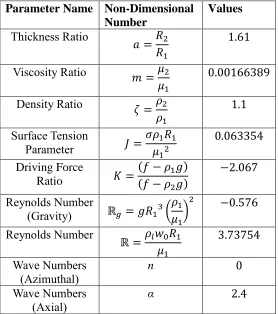
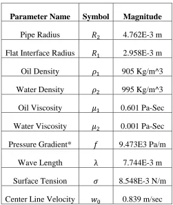
In Chapter 3, ANSYS Fluent code is used to validate a benchmark case simulation results with published work of Li and Renardy (1999) and other experimental results and linear stability analysis. All of the flow parameters for the benchmark case study are taken from Li and Renardy (1999) and experimental set-up of Bai et al. (1992).

In Chapter 4 and 5, the bulk of our new findings are described in detail. Oscillation and modulations of the waves were described for a certain range of flow parameters. A detailed description of the bifurcation of the wave is described from flat interface solution to a travelling wave regime and the branch out to an oscillating and modulated regime. Only a certain range of surface tension parameters and Reynolds numbers were considered to map out the regime.

(48)

20

In Chapter 7, 3-D models of the down-flow is described in detail. Results of the 3-D waves are compared with the pattern selection studies of Renardy (1997). Sensitivity of the change in wave shape were studied for a slight change in Reynolds number and compared with the theoretical study of Renardy (1997). Our ANSYS Fluent 3-D results show the true nature of asymmetric shape of the waves. A novel approach is presented to identify various non-symmetric wave shapes such as corkscrew and snake waves from the simulation results. This kind of full blown 3-D model to simulate non-axisymmetric wave shapes (corkscrew and snake waves) are presented for the first time.

In, Chapter 8, we summarized the new findings from our research.

(49)

21

CHAPTER 2 : Mathematical Formulations

2.1 Governing equations and boundary conditions

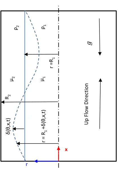
In this chapter, the basics of the core-annular flow of two immisicible fluids passing through a pipeline of circular cross section is presented. The interface between the two fluids could be flat or wavy depending on flow conditons. In this section, a general mathematical formulation of core-annular flow is illustrated.

The schematic diagram of the core-annular flow is depicted in Figure 3. Let us consider cylindrical coordinate system with r, θ, and x as three ordinates. The radius of the pipe is at 𝑟 = 𝑅2. The axis of the pipe is located at 𝑟 = 0. The interface between the two

fluids is defined at 𝑟 = 𝑅₁ + δ(𝜃, 𝑥, 𝑡) . For flat interface problem or basic flow problem, the interface location reduces to 𝑟 = 𝑅₁. The density and viscosity of the core fluid (fluid 1) is denoted as 𝜌₁ and 𝜇_1, and the density and viscosity of the annulus fluid (fluid 2) is denoted as 𝜌₂ and 𝜇₂. Both density and viscosity of the core and annular fluids are considered to be constants. The gravity is acting in the negative x-direction as shown in

(50)

22

Figure 3: Schematic of core-annular flow.

The three components of the conservation of momentum equation in r, θ, and x

directions for both core and annular flow are presented below,

𝜌𝑙[

𝜕𝑢_𝑟

𝜕𝑡 + (𝐮 ∙ 𝛁)𝑢𝑟− 𝑢_𝜃2

𝑟 ] = − 𝜕𝑝 𝜕𝑟+ 𝜇𝑙[𝛻 2_𝑢 𝑟− 𝑢_𝑟 𝑟2 −

2 𝑟2 𝜕𝑢_𝜃 𝜕𝜃 ] + 𝜌𝑙𝑔𝑟, (2.1) 𝜌𝑙[ 𝜕𝑢_𝜃 𝜕𝑡 + (𝐮 ∙ 𝛁)𝑢𝜃+ 𝑢_𝑟𝑢_𝜃 𝑟 ] = − 1 𝑟 𝜕𝑝 𝜕𝜃+ 𝜇𝑙[𝛻 2_𝑢 𝜃− 𝑢_𝜃 𝑟2 +

2 𝑟2 ∂𝑢_𝑟 ∂𝜃] + 𝜌𝑙𝑔θ, (2.2) 𝜌_𝑙[𝜕𝑢𝑥 𝜕𝑡 + (𝐮 ∙ 𝛁)𝑢𝑥] = − 𝜕𝑝 𝜕𝑥+ 𝜇𝑙𝛻 2_𝑢 𝑥+ 𝜌𝑙𝑔𝑥. (2.3)

Here, pressure is represented by 𝑝 and the component of the velocity in the r, θ, and x

directions are represented by𝑢_𝑟, 𝑢_𝜃, and 𝑢_𝑥 respectively. Also, 𝜌_𝑙 and 𝜇_𝑙 are density and dynamic viscosity of fluid 1 (core, 𝑙 =1) and fluid 2 (annulus, 𝑙 =2). Components of the

r =R 1 R2 μ1 μ2

ρ2 ρ1

(51)

23

gravitational acceleration are 𝑔_𝑟, 𝑔_θ and 𝑔_𝑥 respecitvely. For the configuration shown in Figure 3, 𝑔_𝑟 = 0 , 𝑔_θ= 0, and 𝑔_𝑥 = −𝑔. In addition, we define,

𝐮 ∙ 𝛁 = 𝑢_𝑟 𝜕 𝜕𝑟+ 𝑢𝜃 𝑟 𝜕 𝜕𝜃+ 𝑢𝑥 𝜕 𝜕𝑥 , (2.4) and

𝛻2 =1 𝑟 𝜕 𝜕𝑟(𝑟 𝜕 𝜕𝑟) + 1 𝑟2 𝜕2

𝜕𝜃2 +

𝜕2

𝜕𝑥2 .

(2.5)

The momentum equation could also be expressed in a vector form as

𝜌_𝑙[𝜕𝐮

𝜕𝑡 + 𝐮 ∙ 𝛁𝐮] = −𝛁𝑝 + 𝜇𝑙𝛻

2_{𝐮 + 𝜌}

𝑙𝐠.

(2.6)

Similarly, the continuity equation in the cylindrical coordinate could be written as 𝜕𝜌 𝜕𝑡 + 1 𝑟 𝜕 𝜕𝑟(𝜌𝑟𝑢𝑟) + 1 𝑟 𝜕 𝜕𝜃(𝜌𝑢𝜃) + 𝜕

𝜕𝑥(𝜌𝑢𝑥) = 0.

(2.7)

Its vector form could be represented as 𝜕𝜌

𝜕𝑡 + 𝛁 ⋅ (𝜌𝐮) = 0.

(2.8)

In order to present the conditions at the interface, it is convenient to introduce a scalar function F(x(r, 𝜃,x),t). This scalar function describes the interface shape as a set of points that satisfy,

𝐹(𝐱(𝑟, 𝜃, 𝑥), 𝑡) ≡ 0. (2.9)

Essentially, a material particle at the interface will always remain at the interface. Since,

(52)

24 𝜕𝐹

𝜕𝑡 + 𝐮 ∙ 𝛁𝐹 = 0.

(2.10)

From analytical geometry, the unit normal for the inteface surface 𝐹(𝐱(𝑟, 𝜃, 𝑥), 𝑡) = 0 could be defined as

𝐧 = 𝛁𝐹 |𝛁𝐹|.

(2.11)

Equation (2.10) is the most general form of the kinematic condition of the inteface. In this particular problem shown in Figure 3, the interface could be defined as

𝑟 =𝑅₁+ 𝛿(𝜃, 𝑥, 𝑡). (2.12)

Here, 𝛿(𝜃, 𝑥, 𝑡) is the deviation of the interface from the flat one, at 𝑟 =𝑅₁. Therefore, in this case equation (2.9) takes the form,

𝐹 = 𝑟(𝑡) − 𝑅₁− 𝛿(𝜃(𝑡), 𝑥(𝑡), 𝑡) = 0. (2.13)

Using equation (2.13), the kinematic condition (2.10) reduces to,

−𝛿_𝑡+ 𝑢_𝑟− 𝑢_𝜃𝛿_𝜃− 𝑢_𝑥𝛿_𝑥= 0. (2.14)

Similarly, equation (2.11) becomes,

𝐧 =𝒆̂𝑟− 𝛿𝜃𝒆̂𝜽− 𝛿𝑥𝒆̂𝑥 √1 + 𝛿_𝜃2_{+ 𝛿}

𝑥2

. (2.15)

Here, 𝒆̂𝑟, 𝒆̂𝜃, and 𝒆̂𝑥, are unit normals in r, 𝜃, and x direction respectively and 𝛿𝑡,𝛿𝜃 and

𝛿𝑥 are partial derivatives of the deviation 𝛿(𝜃, 𝑥, 𝑡), 𝑖. 𝑒., 𝛿𝑡 = 𝜕𝛿

𝜕𝑡,𝛿𝜃 =

𝜕𝛿

𝜕𝜃, and 𝛿𝑥 = 𝜕𝛿 𝜕𝑥

respectively.

At this point, it is imporatant to introduce a notation of the jump. For any quantity F

(53)

25

⟦𝐹⟧ = 𝐹|_{𝑟= (𝑅}₁_+𝛿)₊− 𝐹|_{𝑟= (𝑅}₁_+𝛿)₋. (2.16)

At any specified point on the interface, the velocity is continuous between the two fluids (no-slip). Therefore,

⟦𝐮⟧ = 0. (2.17)

The surface traction at the interface is balanced by surface forces, or

⟦−𝑝𝐈 + 2𝜇𝐄⟧ ∙ 𝐧 = 𝛁2𝜎 + 𝐻𝜎𝐧. (2.18)

Here, 𝜎 is surface tension and 𝛁₂𝜎 is the surface gradient of surface tension 𝜎, which could be introduced by temperature or concentration gradient along the interface. H is the mean curvature, and 𝐄 is the strain rate tensor,

𝐄 =1

2(𝛁𝐮 + 𝛁𝐮

𝑇_). (2.19)

To complete the mathematical specification of core-annular flow, the boundary conditions at the center of the pipe and at the wall needed to be satisfied,

𝐮 = finite, at 𝑟 = 0, (2.20)

and

𝐮 = 0, (𝑖. 𝑒. , 𝑢_𝑟 = 0; 𝑢_𝜃 = 0; 𝑢_𝑥 = 0), at𝑟 = 𝑅₂. (2.21)

2.2 Base flow

(54)

26

this flat interface or perfect core-annular flow or basic flow problem, the solution of the velocity and pressure fields can be simplified to

𝑢_𝑟 = 0, 𝑢_𝜃 = 0, 𝑢𝑥 = 𝑤(𝑟),

𝑝 = 𝑃(𝑥).

(2.22)

The boundary conditions (2.20) and (2.21) reduce to

𝑤 is finite at 𝑟 = 0, (2.23)

and

𝑤 = 0 at 𝑟 = 𝑅₂, (2.24)

respectively.

For this basic flow, there is no fluctuation of the interface, therefore 𝛿 = 0 and 𝐧 = 𝒆̂_𝑟. At the interface 𝑟 = 𝑅₁, components of the velocities match between the two phases.

Therefore, equation (2.17) reduces to

(𝑤)₁ = (𝑤)₂. (2.25)

Traction condition (2.18) at the inteface could be written as

⟦−𝑃𝐈 + 2𝜇𝐄⟧ ∙ 𝒆̂𝑟 = 𝐻𝜎𝒆̂𝑟. (2.26)

After simplification, equation (2.26) reduces to

⟦−𝑃 + 2𝜇𝐸𝑟𝑟⟧𝒆̂𝑟+ ⟦2𝜇𝐸𝜃𝑟⟧𝒆̂𝜃+ ⟦2𝜇𝐸𝑥𝑟⟧𝒆̂𝒙 = 𝐻𝜎𝒆̂𝑟. (2.27)

Since, 𝑢_𝑟 = 0, and 𝑢_𝜃 = 0, traction condition (2.27) in the axial direction reduces to

⟦𝜇𝑑𝑤 𝑑𝑟⟧ = 0.

(2.28)

(55)

27

⟦−𝑃 + 2𝜇𝐸𝑟𝑟⟧ = 𝐻𝜎. (2.29)

Here, 𝜎 is surface tension and H is simplified curvature defined by H =(1

𝑅1). Therefore, equation (2.29) reduces to

𝑃₂− 𝑃₁ = 𝜎 𝑅1

. (2.30)

Thus, 𝑑𝑃₁/𝑑𝑥 = 𝑑𝑃₂/𝑑𝑥 = 𝑑𝑃/𝑑𝑥 .

After substituting the components of velocity from equation (2.22) to momentum equation (2.2) to (2.3) we obtain the following result

0 = 𝑓 + 𝜇𝑙[

𝑑2𝑤 𝑑𝑟2 +

1 𝑟

𝑑𝑤

𝑑𝑟] − 𝜌𝑙𝑔 .

(2.31)

Here,

𝑓 = − 𝑑𝑃 𝑑𝑥.

(2.32)

Rearranging equation(2.31), we obtain

[1 𝑟

𝑑 𝑑𝑟] [𝑟

𝑑𝑤 𝑑𝑟] = −

(𝑓 − 𝜌𝑙𝑔)

𝜇_𝑙 .

(2.33)

The general solution of equation(2.33)in the core and annulus can be written as,

𝑤(𝑟) =

{

− (𝑓 − 𝜌1𝑔)

4𝜇₁ 𝑟

2_{+ 𝐴}

1𝑙𝑛 𝑟 + 𝐵1 , 0 ≤ 𝑟 ≤ 𝑅1,

− (𝑓 − 𝜌2𝑔) 4𝜇2

𝑟2+ 𝐴2𝑙𝑛 𝑟 + 𝐵2 , 𝑅1 ≤ 𝑟 ≤ 𝑅2.

(2.34)

(56)

28 𝑤(𝑟)

=

{

(𝑓 − 𝜌1𝑔) 4𝜇1

(𝑅12− 𝑟2) +

(𝑓 − 𝜌₂𝑔) 4𝜇2

(𝑅22− 𝑅12) + 𝑅12

(𝜌₁− 𝜌₂)𝑔 2𝜇2

𝑙𝑛𝑅2 𝑅₁ 0 ≤ 𝑟 ≤ 𝑅1 ,

(𝑓 − 𝜌2𝑔)

4𝜇₂ (𝑅2

2_{− 𝑟}2_{) − 𝑅}

12

(𝜌1− 𝜌2)𝑔

2𝜇₂ 𝑙𝑛 𝑟

𝑅₂ 𝑅1 ≤ 𝑟 ≤ 𝑅2.

(2.35)

In order to express the general solution of the base flow in the dimensionlesss form, we may scale the length with the radius of the interface 𝑅₁, and velocity with the center line velocity 𝑤₀. The dimensionless velocity profile for the core and annulus velocity could be expressed as,

𝑤̅ (𝑟̅ ) = 𝑤 𝑤𝑜

= { 1 − 𝑚𝐾 𝑟̅2

Λ 0 ≤𝑟̅ < 1, [𝑎2−𝑟̅2− 2(𝐾 − 1) ln(𝑟̅ /𝑎)]/𝛬 1 ≤𝑟̅ ≤ a.

(2.36)

Here, the dimensionless parameters are,

𝑚 =𝜇2 𝜇₁,

𝜁 =𝜌2 𝜌₁,

𝑎 =𝑅2 𝑅₁,

𝐾 =(𝑓 − 𝜌1𝑔) (𝑓 − 𝜌₂𝑔).

(2.37)

Also, 𝛬 is defined by,

𝛬 = 𝐾𝑚 + 𝑎2− 1 + 2(𝐾 − 1) 𝑙𝑛 𝑎. (2.38)

The centerline velocity 𝑤₀, at 𝑟 = 0 could be obtained from equations (2.35) and (2.38), and could be expressed as

𝑤0 =

(𝑓 − 𝜌₂𝑔) 4𝜇2

𝛬𝑅12.

(57)

29

If the gravity is ignored, i.e., 𝑔 = 0, then the general solution listed in equation (2.35) becomes

𝑤(𝑟) =

{ 𝑓 4𝜇₁(𝑅1

2_{− 𝑟}2_{) +} 𝑓

4𝜇₂(𝑅2

2_{− 𝑅}

12) 0 ≤ 𝑟 ≤ 𝑅1 ,

𝑓 4𝜇2

(𝑅22− 𝑟2) 𝑅1 ≤ 𝑟 ≤ 𝑅2.

(2.40)

The corresponding non-dimensional form of the velocity is

𝑤̅ (𝑟̅ ) =

{

1 − 𝑚 𝑟̅2

(𝑎2 _{+ 𝑚 − 1)} 0 ≤𝑟̅ < 1 ,

𝑎2_−𝑟̅2

(𝑎2_{+ 𝑚 − 1)} 1 ≤𝑟̅ ≤ a.

(2.41)

2.3 Perturbed flow

The basic flow solution with a flat interface described in section 2.2 may not be stable. To determine the stability of the basic flow, it is necessary to perform a linear stability analysis. In order to do that, the basic flow solution is perturbed with a small disturbance such that

𝑢_𝑟 = 0 + 𝓊,

𝑢_𝜃 = 0 + 𝓋,

𝑢𝑥 = 𝑤(𝑟) + 𝓌,

𝑝 = 𝑃 + 𝓅,

(2.42)

and the interface is at,

𝑟 = 𝑅₁+ 𝛿(𝜃, 𝑥, 𝑡). (2.43)

(58)

30

dropping the terms related to the basic flow, and neglecting multiplication terms of two small quantities, we obtain the following linearized governing equations in terms of 𝓊, 𝓋, 𝓌, and 𝓅.

𝜌𝑙[ 𝜕𝓊 𝜕𝑡 + 𝑤 𝜕𝓊 𝜕𝑥] = − 𝜕𝓅 𝜕𝑟 + 𝜇𝑙[𝛻

2_{𝓊 −} 𝓊

𝑟2−

2 𝑟2 𝜕𝓋 𝜕𝜃], (2.44) 𝜌_𝑙[𝜕 𝓋 𝜕𝑡 + 𝑤 𝜕 𝓋 𝜕𝑥] = − 1 𝑟 𝜕𝓅 𝜕𝜃 + 𝜇𝑙[𝛻

2_{𝓋 −} 𝓋

𝑟2 +

2 𝑟2 𝜕𝓊 𝜕𝜃], (2.45) 𝜌_𝑙[𝜕𝓌 𝜕𝑡 + 𝑤 𝜕𝓌 𝜕𝑥 + 𝑤 ′_{𝓊] = −}𝜕𝓅 𝜕𝑥 + 𝜇𝑙𝛻

2_𝓌. (2.46)

Similarly, the continuity equation (2.4) reduces to 1 𝑟⋅ 𝜕 𝜕𝑟(𝑟𝓊) + 1 𝑟 𝜕𝓋 𝜕𝜃 + 𝜕𝓌 𝜕𝑥 = 0.

(2.47)

The boundary condition listed in equation (2.20) and equation (2.21) become

𝓊,𝓋, and𝓌 are finite, at 𝑟 = 0, (2.48)

and

𝓊 = 𝓋 = 𝓌 = 0 at 𝑟 = 𝑅₂ , (2.49)

respectively.

For the perturbed flow, the interface is located at 𝑟 = 𝑅1+ 𝛿. However, it is

convenient to apply the interface conditions at the unperturbed location, 𝑟 = 𝑅₁. This requires the use of Taylor series expansion for any quantity F near the interface

𝐹|_{𝑟 = 𝑅}₁_+𝛿 ≈ 𝐹|_{𝑟 = 𝑅}₁ + 𝛿𝜕𝐹

𝜕𝑟|𝑟 = 𝑅1.

(2.50)

(59)

31

𝓊 = 𝛿_𝑡+ 𝛿_𝑥𝑤 . (2.51)

Similarly, velocity conditions at 𝑟 = 𝑅1,

⟦𝓊⟧ = 0, ⟦𝓋⟧ = 0,

⟦𝓌⟧ + 𝛿⟦𝑤′_{⟧ = 0.}

(2.52)

Shear traction at the interface 𝑟 = 𝑅₁+ 𝛿 is obtained by 𝜃 and x component of equation (2.27). We also need to use the equation (2.50) and equation (2.16). After neglecting the multiplication of two small terms and dropping ⟦𝜇𝑙𝑤′⟧ = 0 at 𝑟 = 𝑅1, we

obtain the following shear traction condition at the interface 𝑟 = 𝑅1,

⟦𝜇 (𝜕𝓊 𝜕𝑥 +

𝜕𝓌

𝜕𝑟)⟧ + 𝛿⟦𝜇𝑤

′′_{⟧ = 0,} (2.53)

and

⟦𝜇 (𝜕𝓊 𝜕𝜃 + 𝑅1

𝜕𝓋

𝜕𝑟 − 𝓋)⟧ = 0.

(2.54)

Similarly, normal traction (r component of equation (2.27)) condition at the interface reduces to

−⟦𝓅⟧ + 2 ⟦𝜇𝜕𝓊 𝜕𝑟⟧ =

𝜎 𝑅12

(𝛿 + 𝛿𝜃𝜃+ 𝑅12𝛿𝑥𝑥).

(2.55)

Here, the curvature of the interface is defined by 𝐻 =(𝛿+𝛿𝜃𝜃+𝑅12𝛿𝑥𝑥)

(60)

32

2.4 Dimensionless equations for the perturbed flow

From here on, we will discuss the equation and boundary conditions in the dimensionless form. We will use the same notation for the dimensionless variables in our discussion without much confusion.

Here, we introduce a few additional non-dimensional parameters such as Reynolds number and surface tension parameters. Reynolds number is defined as

ℝ𝑙 =

𝜌_𝑙𝑤₀𝑅₁ 𝜇𝑙

, 𝑙 = 1, 2 ; (or ℝ1 = ℝ. )

(2.56)

The surface tension parameter is defined as

𝑆 = 𝜎

𝜌₁𝑤₀2_𝑅 1

. (2.57)

The surface tension parameter, 𝑆 , strongly depends upon center line velocity. An alternative surface tension parameter is defined by 𝐽, which is independent of centerline velocity,

𝐽 = 𝜎𝑅1 𝜌₁𝜈₁2 =

𝜎𝑅₁ 𝜇₁2 𝜌1 .

(2.58)

𝐽 and 𝑆 are related by 𝑆 = 𝐽

ℝ12. In our analysis we used the surface tension parameter 𝐽 which is shown in equation (2.58).

Hu and Patankar (1995) defined ℝ_𝑔 , a non-dimensional Reynolds number for vertical

core-annular flow

ℝ𝑔 = 𝑔𝑅13(

𝜌₁ 𝜇1

)

2

(61)

33

ℝ_𝑔 is co-related with non-dimensional quantity with the driving force𝐾 listed in equation

(2.37) and with other dimensionless numbers such as ℝ, 𝑚, 𝑎, and 𝜁 by the following equation,

𝐾 =4𝑚ℝ − (𝜁 − 1)ℝ𝑔(𝑎

2_{− 1 − 2 𝑙𝑛 𝑎)}

4𝑚ℝ + (𝜁 − 1)ℝ𝑔(𝑚 + 2 𝑙𝑛 𝑎)

. (2.60)

For upward flow, ℝ_𝑔 is negative and for downward flow the value of ℝ_𝑔 is positive. For

horizontal pipe flow with equal densities, ℝ_𝑔 = 0.

Now let us scale the velocities (𝓊, 𝓋, 𝓌) with 𝑤𝑜, length (𝑥, 𝑟) with 𝑅1, time with

𝑅1

𝑤𝑜

and pressure with 𝜌𝑙𝑤𝑜2 . In this way, the governing equations, (2.44)to (2.47) reduce to

[𝜕𝓊 𝜕𝑡 + 𝑤̅ 𝜕𝓊 𝜕𝑥] = − 𝜕𝓅 𝜕𝑟 + 1 ℝ_𝑙[𝛻

2_{𝓊 −} 𝓊

𝑟2−

2 𝑟2 𝜕𝓋 𝜕𝜃], (2.61) [𝜕 𝓋 𝜕𝑡 + 𝑤̅ 𝜕 𝓋 𝜕𝑥] = − 1 𝑟 𝜕𝓅 𝜕𝜃 + 1 ℝ_𝑙[𝛻

2_{𝓋 −} 𝓋

𝑟2+

2 𝑟2 𝜕𝓊 𝜕𝜃] (2.62) [𝜕𝓌 𝜕𝑡 + 𝑤̅ 𝜕𝓌 𝜕𝑥 + 𝑤̅ ′_{𝓊] = −}𝜕𝓅 𝜕𝑥 + 1 ℝ𝑙

𝛻2𝓌 , (2.63)

and 1 𝑟⋅ 𝜕 𝜕𝑟(𝑟𝓊) + 1 𝑟 𝜕𝓋 𝜕𝜃 + 𝜕𝓌 𝜕𝑥 = 0.

(2.64)

It is observed that, the non-dimensional form of the equations are obtained by substituting 𝜌_𝑙= 1 and 𝜇_𝑙 by 1/ℝ_𝑙.

Interfacial Wave Dynamics Of Core-Annular Flow Of Two Fluids

ScholarlyCommons

Interfacial Wave Dynamics Of Core-Annular Flow

Of Two Fluids

Interfacial Wave Dynamics Of Core-Annular Flow Of Two Fluids

INTERFACIAL WAVE DYNAMICS OF CORE-ANNULAR

FLOW OF TWO FLUIDS

INTERFACIAL WAVE DYNAMICS OF CORE-ANNULAR

FLOW OF TWO FLUIDS

©COPYRIGHT

2018

ABSTRACT

INTERFACIAL WAVE DYNAMICS OF CORE-ANNULAR FLOW OF

TWO FLUIDS

TABLE OF CONTENTS

CHAPTER 1

: Introduction

CHAPTER 2

: Mathematical Formulations