www.nat-hazards-earth-syst-sci.net/17/45/2017/ doi:10.5194/nhess-17-45-2017
© Author(s) 2017. CC Attribution 3.0 License.
Coastal ocean forecasting with an unstructured grid model in the
southern Adriatic and northern Ionian seas
Ivan Federico1, Nadia Pinardi1,2,3, Giovanni Coppini1, Paolo Oddo2,a, Rita Lecci1, and Michele Mossa4
1Centro Euro-Mediterraneo sui Cambiamenti Climatici – Ocean Predictions and Applications, via Augusto Imperatore 16,
73100 Lecce, Italy
2Istituto Nazionale di Geofisica e Vulcanologia, Via Donato Creti 12, 40100 Bologna, Italy 3Universitá degli Studi di Bologna, viale Berti-Pichat, 40126 Bologna, Italy
4Dipartimento di Ingegneria Civile, Ambientale, del Territorio, Edile e di Chimica, Politecnico di Bari, Via E. Orabona 4,
70125 Bari, Italy
anow at: NATO Science and Technology Organisation – Centre for Maritime Research and Experimentation,
Viale San Bartolomeo 400, 19126 La Spezia, Italy
Correspondence to:Ivan Federico (ivan.federico@cmcc.it)
Received: 13 May 2016 – Published in Nat. Hazards Earth Syst. Sci. Discuss.: 25 May 2016 Accepted: 6 December 2016 – Published: 11 January 2017
Abstract. SANIFS (Southern Adriatic Northern Ionian coastal Forecasting System) is a coastal-ocean operational system based on the unstructured grid finite-element three-dimensional hydrodynamic SHYFEM model, providing short-term forecasts. The operational chain is based on a downscaling approach starting from the large-scale system for the entire Mediterranean Basin (MFS, Mediterranean Forecasting System), which provides initial and boundary condition fields to the nested system.
The model is configured to provide hydrodynamics and active tracer forecasts both in open ocean and coastal waters of southeastern Italy using a variable horizontal resolution from the open sea (3–4 km) to coastal areas (50–500 m).
Given that the coastal fields are driven by a combination of both local (also known as coastal) and deep-ocean forc-ings propagating along the shelf, the performance of SAN-IFS was verified both in forecast and simulation mode, first (i) on the large and shelf-coastal scales by comparing with a large-scale survey CTD (conductivity–temperature–depth) in the Gulf of Taranto and then (ii) on the coastal-harbour scale (Mar Grande of Taranto) by comparison with CTD, ADCP (acoustic doppler current profiler) and tide gauge data.
Sensitivity tests were performed on initialization condi-tions (mainly focused on spin-up procedures) and on surface boundary conditions by assessing the reliability of two
al-ternative datasets at different horizontal resolution (12.5 and 6.5 km).
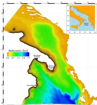
Figure 1.SANIFS domain: horizontal grid overlapped on bathymetry for the whole domain.
1 Introduction
Many human activities are concentrated in coastal areas where traditional resource-based activities, such as coastal fisheries and aquaculture, coexist with urban development, port traffic and tourism. The management of such a com-plex area at the interface between land and ocean environ-ments, requires numerical modelling and predictive capabil-ities that are now possible due to the availability of large-scale ocean forecasts and analyses used to initialize coastal models that downscale and increase the accuracy of fore-casts near the coasts (Pinardi et al., 2003; Pinardi and Cop-pini, 2010). Furthermore, ocean operational forecasting con-tributes greatly to the understanding of ocean dynamics and provide an efficient support tool for marine environmental management (Oddo et al., 2006; Robinson and Sellschopp, 2002). In particular, a high-resolution operational forecasting system could contribute to making decisions for mitigation of natural hazards in coastal areas, such as storm surge events, minimizing their potential negative impacts on a wide range of coastal and maritime facilities and reducing the damages to coastal communities.
The main objective of the present work is to highlight how downscaling can improve the simulation of the flow field, going from typical open-ocean scales of the order of several kilometres to the coastal (and harbour) scales of tens to hdreds of metres. Two methodologies were adopted: 3-D un-structured grid modelling and a downscaling approach that uses open-ocean fields as initial and lateral boundary condi-tions.
Classical ocean models are based on finite difference schemes on Cartesian grids (Griffies et al., 2000). It is only in the last decade that unstructured mesh methods have been used more intensively in ocean and coastal modelling, adopt-ing both finite elements (e.g. Umgiesser et al., 2004; Danilov et al., 2004; Walters, 2005; Le Bars et al., 2010) and finite volume (e.g. Casulli and Zanolli, 2000; Chen et al., 2003; Ham et al., 2005; Fringer et al., 2006) discretization. Un-structured grid models are used for coastal modelling, ex-ploiting their efficiency at handling complex coastlines while not neglecting large-scale processes.
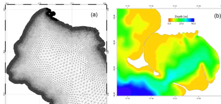
Figure 2.Enlarged views of horizontal grid Gulf of Taranto(a)and bathymetry in Mar Grande of Taranto(b).
(Kourafalou et al., 2015). Here the downscaling was per-formed from the Mediterranean scale through a one-way nesting approach with the Mediterranean Forecasting System (MFS) numerical model (Oddo et al., 2014). The nested un-structured grid system was built on a resolution higher than MFS both horizontally and vertically over the entire open ocean and coastal domain.
Unstructured grid and downscaling approaches were in-corporated to build the very-high-resolution operational sys-tem SANIFS (Southern Adriatic Northern Ionian coastal Forecasting System), which produces short-term forecasts and is constantly under development.
The specific coastal area studied in this paper is the south-ern Adriatic, northsouth-ern Ionian (SANI) area (Fig. 1), with a par-ticular focus on the Gulf of Taranto and Mar Grande (Fig. 2). The southern Adriatic Sea extends approximately southward along the latitude of 42◦N to the threshold of the Strait of Otranto and has a maximum depth of 1270 m. An exchange of waters with the Ionian Sea occurs at the Strait of Otranto at approximately 40◦N. The northern Ionian Sea extends south of 38◦N and has a steeper continental slope than the Adriatic basin. The offshore maximum depth is 3500–3700 m.
The Gulf of Taranto is situated in the northwestern Io-nian Sea and is approximately delimited in open sea by the line connecting Cape Santa Maria di Leuca (in Apu-lia) and Cape Colonna (see Fig. 1). A complex water mass circulation (Sellschopp and Álvarez, 2003) with high sea-sonal variability (Milligan and Cattaneo, 2007) characterizes the Gulf of Taranto basin. Oceanographic studies (Poulain, 2001; Bignami et al., 2007; Turchetto et al., 2007; Grauel and Bernasconi, 2010; Oddo and Guarnieri, 2011) based on interannual simulations describe two main Gulf of Taranto surface circulation structures: (i) a cyclonic gyre encompass-ing the Western Adriatic Coastal Current (WACC) flowencompass-ing around Apulia into the Taranto Gulf from the northern Adri-atic Sea, and (ii) an anticyclonic circulation connected to the
Ionian Surface Waters (ISW) flow entering from the central Ionian Sea. In addition, studies on the coastal current in the inner part of the Gulf of Taranto (De Serio and Mossa, 2015a) show a coastal flow supporting the anticyclonic gyre struc-ture. In the Mar Grande of Taranto (Fig. 2b) the circulation consists of along-shore currents, which follow the direction of the wind and are modulated by tidal forcing (Scroccaro et al., 2004) with a tidal range of about 20 cm (Umgiesser et al., 2014).
A regional cruise, called MREA14 (Maritime Rapid Envi-ronmental Assessment in 2014), was carried out in the Gulf of Taranto in October 2014 in order to provide data for vali-dating the SANIFS downscaled simulations. Thus, the SAN-IFS system has been fully validated for the time period of the available data, both on regional and coastal scales.
The paper is organized as follows. In Sect. 2 the design and implementation of the forecasting system are introduced. Section 3 reports the sensitivity experiments and the valida-tion of the SANIFS system. Secvalida-tion 4 discusses the circula-tion structures emerging from the SANIFS system during the validation exercise, and concluding remarks are provided in Sect. 5.
2 The forecasting system: definition and implementation
Table 1.Configuration of the SANIFS system.
SANIFS (Southern Adriatic Northern Ionian coastal Forecasting System) configuration
Model SHYFEM (Umgiesser et al., 2004)
Horizontal resolution Open sea: 3–4 km
Coastal area: 500–50 m
Vertical resolution Number of levels: 99
The layer thickness is 2 until 40 m from surface;
then progressively (stepwise) increased down to the bottom
Vertical mixing Pacanowski and Philander (1981) scheme modified by Lermusiaux (2001)
Bottom friction Non-linear bottom parameterization assuming a quadratic bottom friction;
drag coefficient calculated by Maraldi et al. (2013)
Initial condition fields Ocean: temperature, salinity, sea level and currents from MFS
Lateral open boundary condition fields Ocean: temperature, salinity, non-tidal sea level and total currents from MFS
Tides: tidal elevation from OTPS
Rivers River runoffs: 20 monthly mean climatologies
Atmospheric forcing ECMWF or COSMOME
Spin-up time 3 days
adopted by other forecasting systems downscaled from MFS, as reported in Napolitano et al. (2016).
In this section we report the main model settings, the sur-face boundary conditions, lateral boundary conditions and the operational configuration. These are summarized in Ta-ble 1.
2.1 Model settings
The SANIFS forecasting system is based on the SHYFEM model, which is a 3-D finite element hydrodynamic model (Umgiesser et al., 2004; Cucco and Umgiesser, 2006) solving the Navier–Stokes equations by applying hydro-static and Boussinesq approximations. The unstructured grid is Arakawa B with triangular meshes (Bellafiore and Umgiesser, 2010; Ferrarin et al., 2013), which provides an accurate description of irregular coastal boundaries. The scalars are computed at grid nodes, whereas velocity vec-tors are calculated at the centre of each element. Verti-cally a z layer discretization is applied and most variables are computed in the centre of each layer, whereas stress terms and vertical velocities are solved at the layer inter-faces (Bellafiore and Umgiesser, 2010). In the coastal waters of the eastern Italian coastlines, the model has a high spa-tial resolution, generally reaching an element size of 500 m, with further refinements in specific areas (e.g. Mar Grande of Taranto, Fig. 2b) where the resolution reaches 50 m. In the open-ocean areas, the horizontal resolution is approxi-mately 3–4 km, compared to the 6–7 km of the parent model. The SANIFS bathymetry (Figs. 1 and 2b) was derived from the US Digital Bathymetric Data Base Variable Resolutions
(DBDB-1) at 10 resolution for the Mediterranean Basin and integrated with higher-resolution bathymetry for coastal ar-eas in the Gulf of Taranto provided by the Italian Navy Hy-drographic Institute. The vertical discretization has 99 lev-els. This is appropriate for solving the field both in coastal and open-sea areas. The vertical spacing is 2 m until 40 m from the sea surface, and the resolution is then progressively (stepwise) increased down to the bottom with a maximum layer thickness of 200 m.
A non-linear bottom parameterization assuming a quadratic bottom friction was imposed. The friction coeffi-cient was expressed asR=CDpu2+v2+eb, whereuand v are the horizontal velocities, CD is the drag coefficient
calculated by a logarithmic formulation (Maraldi et al., 2013), and eb is the bottom turbulent kinetic energy due
to tides, internal wave breaking and other short timescale currents. Following the Treguier’s 1992 experiment and the MFS settings, eb was set to a value of 2.5×10⁻³m2s−2
(Tréguier, 1992) .
A local Richardson-number-dependent formulation was applied for the vertical momentum and tracer eddy coeffi-cients with a specific constraint in the mixing layer (Ler-musiaux, 2001). Using a scheme similar to Pacanowski and Philander (1981), the calculation of eddy viscosities and diffusivities are based on the Richardson numberRi=
N2/(∂U /∂z)2, where N2 is Brunt–Väisälä frequency and
U (x, y)is the velocity field.
IfRi(x, y, z, t )≥0, the eddy viscosity and diffusivity are set toAv=Abv+(v0)/(1+5Ri)2andKv=Kvb+(v0)/(1+
ad-justment is adopted (Av=5×10⁻³m2s−1 and Kv=5×
10−3m2s−1).
The background molecular coefficients are
Avb=10−6m2s−1 and Kvb=10−7m2s−1. The shear eddy viscosity isν0=5×10⁻³m2s−1. An enhancement in
the mixing layer (Lermusiaux, 2001) was adopted to transfer and dissipate the wind stress and the buoyancy fluxes. The vertical eddy coefficients within the Ekman depthhe(x, y, t )
were set to empirical values calibrated for region and season (Aev=1.5×10⁻³m2s−1 and Kve=5×10⁻⁴m2s−1). The Ekman depth was calculated as a function of turbulent fric-tion velocity u∗(x, y)=√|τ|/ρ0 through the relationship
he=Eku∗/f0, where τ is the wind stress vector, ρ0 the
reference density,f0the Coriolis factor andEkan empirical
coefficient set to 0.7.
2.2 Surface boundary conditions
Four basic surface boundary conditions are used:
1. For temperature, the air–sea heat flux is parameterized by bulk formulas described in Pettenuzzo et al. (2010). 2. For momentum, surface stress is computed with the
wind drag coefficient according to Hellermann and Rosenstein (1983).
3. For the free surface, a water flux is used containing evaporation minus precipitation and runoff.
4. For salinity, the turbulent salt flux is set equal to the product of the water flux and the surface salinity. We considered the 20 monthly mean climatological river runoffs (Verri et al., 2017) of
– Italian Ionian Sea rivers: Basento, Bradano, Crati, Sinni, Agri, Neto;
– Italian Adriatic Sea rivers: Fortore, Cervaro, Ofanto; – Greek Ionian Sea rivers: Arachthos, Thyamis;
– Albania–Montenegro–Croatia Adriatic Sea rivers: Vi-jose, Seman, Shkumbi, Erzen, Ishm, Mat, Drin, Bojana, Neretva.
River inflow surface salinity values were fixed to a con-stant value of 15 psu next to the river mouths, following the sensitivity tests carried out with the MFS parent model and the results of sensitivity tests performed by Simoncelli et al. (2011) on the basis of salinity profiles measured in the shelf areas close to river outlets. This value has also been adopted in other studies on the Adriatic circulation, giving a realistic salinity profile for the open sea (Oddo et al., 2005). Two alternative atmospheric forcing datasets were used in order to set up two SANIFS operational configu-rations (see Sect. 2.4), one forced via ECMWF (European
Centre for Medium Weather Forecasts) products with 6 h fre-quency and 12.5 km horizontal resolution, the other via COS-MOME (based on COSMO model and operated by the Ital-ian National Center of Meteorology and Climatology, CN-MCA) products with 3 h frequency and 6.5 km horizontal resolution. The atmospheric forcing fields used from the two datasets are 2 m air temperature (T2M), 2 m dew point tem-perature (D2M), total cloud cover (TCC), mean sea level at-mospheric pressure (MSL), and meridional and zonal 10 m wind components (U10M and V10M). In the configuration forced by ECMWF data, the total precipitation (TP)-rate data are extracted from the CMAP (CPC, Climate Prediction Cen-ter, Merged Analysis of Precipitation) monthly dataset with a horizontal resolution of 2.5◦×2.5◦. In the configuration forced by COSMOME data, TP derives from the operational COSMOME dataset and is identified as a sum of large-scale precipitation (LSP) and convective precipitation (CP).
Finally, the atmospheric forcing fields were corrected by land-contaminated points following Kara et al. (2007) and horizontally interpolated at each ocean grid node by means of Cressman’s interpolation technique (Cressman, 1959). 2.3 Lateral open boundary conditions
SANIFS is nested in MFS through the two lateral open boundaries (Fig. 1) located at the southern (horizontal bound-ary) and northern (oblique boundbound-ary) parts of the domain. The current MFS implementation is based on NEMO (Nu-cleus for European Modelling of the Ocean, Madec (2008)) finite-difference code with a horizontal resolution of 1/16 of a degree (6–7 km approximately) and 72 unevenly spaced vertical levels. The forecasting system is provided by a data assimilation system based on the 3D-VAR scheme developed by Dobricic and Pinardi (2008).
The scalar MFS fields (non-tidal sea surface height, tem-perature and salinity) are imposed at the SANIFS bound-ary nodes, whereas the MFS total velocities are specified in the barycentre of the triangular elements with two nodes at-tached to the boundaries. The tidal elevation derived from the OTPS (Oregon State University Tidal Prediction Soft-ware (Egbert and Erofeeva, 2002)) tidal model are prescribed at each boundary nodes. Eight of the most significant con-stituents are considered: M2, S2, N2, K2, K1, O1, P1, Q1. 2.4 The operational configuration
!)#'!$#! $ " "" )* !& "" !
Climatology data set (C-MAP)
# '!!&- &# "$ "$ !)##! $ "" -'!-2+2++ 10+10+ ( ^ƉĂĂůƌĞƐ͗ϭϮ͘ϱŬŵʹdŝŵĞƌĞƐ͗ϲŚ !)##! $ "" -'!-2+2+++ 10+10+ ( ^ƉĂĂůƌĞƐ͗ϲ͘ϱŬŵʹdŝŵĞƌĞƐ͗ϯŚ 3(!"#", ++"'++, &!((, #!#, 3(!"#", ++"'++, &!((, #!#, #( data set .-/ ! (a) (b)
1, 1- 1.
'-Days
'"
'','1, '1- '1.
'
'
'-' '
COSMOME - an ', ,-%++ ++%++ ('. '.
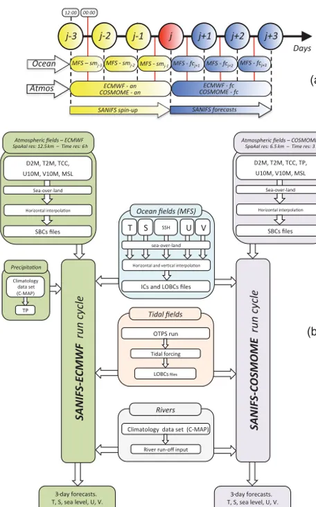
-Figure 3. SANIFS daily forecast cycle (a) and operational
chain(b).
simulations (forj−2 andj−1) and the MFS forecasts (for
j+1, j+2 and j+3) at the lateral open boundary, while the surface boundary conditions run over the ECMWF and COSMOME analysis (j−3,j−2,j−1) and ECMWF and COSMOME forecasts (j+1,j+2,j+3). The forecast is prepared and run automatically. The operational chain is ac-tivated as soon as the atmospheric forcings are available. The technical procedures (Fig. 3b) through scripts and codes for computing the forecast fields can be summarized in the pre-processing of input data, model run and post-pre-processing of the output model.
3 Sensitivity experiments, validation and discussion 3.1 The validation dataset
Three cruises (MREA14) were organized together with data acquisition in the Gulf of Taranto and Mar Grande (Pinardi et al., 2016, in this issue). Data available for the validation
are: (i) temperature and salinity profiles from CTD stations (Fig. 4) and (ii) hourly temperature measurements, sea level and currents at a fixed station (P1 station in Fig. 4, described in De Serio and Mossa, 2015b). The first CTD survey was carried out between 1 and 3 October 2014 and CTDs were acquired on large scales (labelled LS1 in Fig. 4). The second set of surveys was carried out between 5–8 October 2014 at the shelf-coastal (labelled SCS in Fig. 4) and coastal-harbour scales (labelled CHS in Fig. 4) in Mar Grande. The last large-scale survey (labelled LS2 in Fig. 4) completes the mapping of the circulation between 8 and 11 October 2014. The main purpose of the large-scale surveys was to identify the main thermohaline structures in the Gulf of Taranto and to pro-vide an initialization (LS1) and forecast verification survey (LS2). The SCS and CHS surveys focused on the coastal structures and the water exchange between the open sea and Mar Grande.
3.2 Initialization procedure and spin-up time
Limited-area ocean models may require a spin-up time to produce dynamically adjusted fields after initialization from the interpolation of coarser ocean model fields (Simoncelli et al., 2011). Two main issues are addressed here: (i) the dy-namical adjustment at the coasts where coarser ocean fields are extrapolated from the initial conditions and (ii) the sensi-tivity of the initialization to a different number of dynamical fields.
All the experiments were initialized from daily mean fields produced by the MFS parent model. An extrapolation proce-dure (De Dominicis et al., 2013) is used to prevent the pres-ence of missing values interpolating the oceanic fields over the new higher-resolution grid. Two experiments are used: the first (SANIFS-v0) considers the nested model initialized only with temperature and salinity fields from MFS. In the second experiment (SANIFS-v1), the initialization uses tem-perature and salinity, sea level, and currents. Each of these experiments was started at different times with respect to a target initial forecast time. The number of days in the past with respect to the target initial forecast day is called the spin-up time and our aim was to test how long the spin-up needed to be in order to get closer to the observations in the initial condition. The target forecast initial conditions day was 8 October 2014 and the spin-up time was evaluated up to 5 days in the past. A spin-up time indicator is defined as the total kinetic energy (TKE) (Simoncelli et al., 2011) ratio between the parent (MFS) and nested models (SANIFS). In our case this was calculated for the Gulf of Taranto both at the large and shelf-coastal scales.
Figure 4.Sampling strategy of MREA2014 on the three scales. All the circle points refer to CTD stations. P1 refers to the fixed monitoring station in Mar Grande with CTD, ADCP and tidal measures. The MREA timeline is also reported.
(curve plateau or at least a lower gradient of curve) for both experiments is reached after 2 days and kept quasi-constant on the subsequent spin-up days. On the shelf-coastal scale (Fig. 5b), the TKE ratio for different spin-up days has the same qualitative behaviour as the one at the large scale. In order to understand which model initialization fields are re-quired, the model output was compared with the sea surface temperature (SST) observations from satellites in the Gulf of Taranto. Figure 5c shows the root mean square error (RMSE) statistics as a function of spin-up time for SANIFS-v0 and SANIFS-v1. For both model configurations, there is a de-crease in RMSE after 2 days, but SANIFS-v1 is better than SANIFS-v0.
Finally, a further experiment in forecast mode was per-formed focusing on the coastal-harbour scale (Mar Grande of Taranto) and compared with hourly velocity measurements at station P1 (Fig. 4). Figure 5d confirms that SANIFS-v1 ini-tialization has the lowest bias error.
A spin-up time of 3 days appears to be a reasonable choice to ensure the development of internal dynamics by the nested model. This choice was adopted also by other authors imple-menting high-resolution models in re-initialized mode both on large and coastal scale (Rolinski and Umgiesser, 2005; Cucco et al., 2012; Trotta et al., 2016) and also on the har-bour scale (Gaeta et al., 2016, in this issue). We conclude that a spin-up period of 3 days combined with active trac-ers and hydrodynamic initialization is the optimal choice for SANIFS initialization.
3.3 Forecast validation on large, shelf-coastal and coastal-harbour scales
This section investigates the SANIFS forecasting skills at a lead-time of 1 day on the large shelf-coastal and coastal-harbour scales, using the MREA14 observations and in com-parison with MFS. In order to assess the SANIFS forecasting skills using ECMWF atmospheric forcing, the following ex-periments, as reported in Fig. 6, were run: (i) FC-1, FC-2 and FC-3 for LS1 (1–3 October), (ii) FC-4 for CHS (5 October),
sp1 sp2 sp3 sp4 sp5
0.3 0.4 0.5 0.6 0.7 TKE SANIFS / TKE MFS
sp1 sp2 sp3 sp4 sp50.8
0.85 0.9 0.95 1 1.05 1.1 1.15
SANIFS−v0
SANIFS−v1
LS
sp1 sp2 sp3 sp4 sp5
0.4 0.6 0.8 1 1.2 1.4 TKE SANIFS / TKE MFS
sp1 sp2 sp3 sp4 sp50.9
1 1.1 1.2 1.3 1.4 1.5 1.6
SANIFS−v0 SANIFS−v1
SCS
sp1 sp2 sp3 sp4 sp5
0.3 0.35 0.4 0.45
Temperature RMSE (
oC)
Spin−up time (days)
SANIFS−v0
SANIFS−v1
Spin-‐up (me (days)
sp1 sp2 sp3 sp4 sp5
0.4 0.6 0.8 1 1.2 1.4 TKE SANIFS / TKE MFS
sp1 sp2 sp3 sp4 sp50.9
1 1.1 1.2 1.3 1.4 1.5 1.6
SANIFS−v0 SANIFS−v1
sp1 sp2 sp3 sp4 sp5
0.3 0.35 0.4 0.45
Temperature RMSE (
oC)
Spin−up time (days)
SANIFS−v0
SANIFS−v1
sp1 sp2 sp3 sp4 sp5
0.3 0.35 0.4 0.45
Temperature RMSE (
oC)
Spin−up time (days)
SANIFS−v0
SANIFS−v1
(a)
(b)
(c)
2.5 3.5 4.5 0 0.02 0.04 0.06 0.08 0.1
Velocity RMSE (m/s)
SANIFS−v0 SANIFS−v1
fc1 fc2 fc3
V el o ci ty B IA S ( m s )
Forecast days
(d)
-1
Figure 5.TKE ratio between downscaled model (SANIFS) and par-ent model (MFS) as function of spin-up time, calculated on the large
scale LS(a)and shelf-coastal scale SCS(b). Temperature RMSE
(model vs. satellite SST) in the Gulf of Taranto as a function of
spin-up time(c). Velocity bias (m s−1) calculated against hourly
veloc-ities measured at station P1 (Fig. 4) in Mar Grande of Taranto(d).
29 Sep 30 Sep
30 Sep 1 Oct
1 Oct
2 Oct
1 Oct 2 Oct
3 Oct 4 Oct
3 Oct
5 Oct
6 Oct 7 Oct
7 Oct 8 Oct
8 Oct
9 Oct
8 Oct 9 Oct
9 Oct 10 Oct
10 Oct
11 Oct
FC-‐1
FC-‐2
FC-‐3
FC-‐4
FC-‐5
FC-‐6
FC-‐7
FC-‐8
LS1
CHS
SC
S
LS2
Forecast experiments
1 day lead Bme forecast runs over atmospheric forecast Spin-‐up days run over
atmospheric analysis
28 Sep
29 Sep
30 Sep
2 Oct
5 Oct
6 Oct
7 Oct
8 Oct
-
-Figure 6.Sketch of forecast experiments performed on the different scales. The 3 days of spin-up define the initial conditions for the 1-day lead-time forecast.
(iii) 5 for SCS (8 October), and (iv) 6, 7 and FC-8 for LS2 (9–11 October). For each run 3 days of spin-up define the initial conditions for the 1 day lead-time forecast. The LS1 observations were assimilated in MFS to improve forecasts of LS2, SCS and CHS.
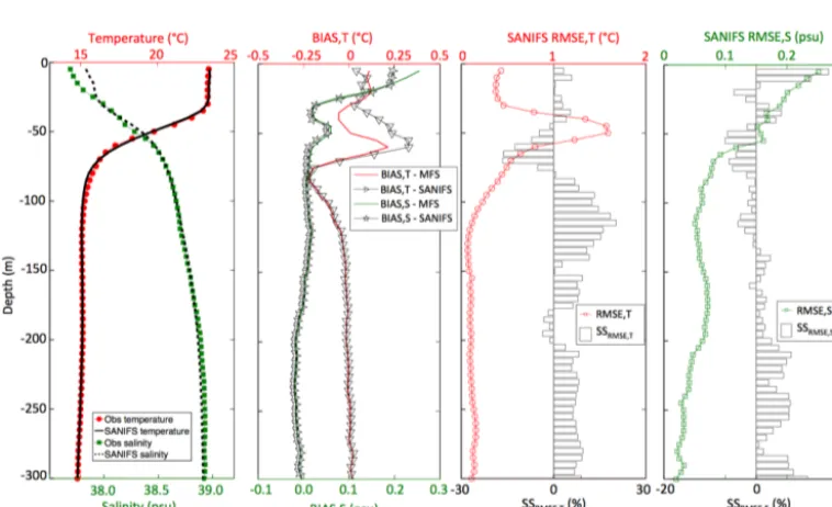
Figure 7 refers to the SANIFS forecasting skills at LS1. In particular, Fig. 7a reports the comparison between mod-elled and observed representative profiles of temperature and salinity obtained by averaging all the LS1 stations. The ob-served temperature profile is well reproduced by the model in the mixed layer, while the model thermocline is shifted up-wards by about 10 m in respect to the observed one, suggest-ing that future model investigations should address the im-provement of the vertical mixing processes. Figure 7b shows the bias of the average profiles compared with the observa-tions. For the salinity field, the higher discrepancies in the ob-servations were found on the surface with a bias of 0.80 psu and could indicate the impact of atmospheric uncertainties of precipitation in the parent model affecting the SANIFS initial condition. However, this discrepancy in surface between the model and observations is lower than the one between MFS and observations. Figure 7c–d show the SANIFS RMSE (red line with circles for temperature and green line with squares
for salinity) and the RMSE skill score in respect to the refer-ence model MFS forecasts (histograms), calculated as
SSRMSE,φ=100
RMSEMFS,φ−RMSESANIFS,φ
RMSEMFS,φ
[%], (1) whereφindicates temperature and salinity. This expression identifies the percentage improvement (positive values) or worsening (negative values) of the SANIFS forecast in com-parison with the MFS ones. The slight improvement of the SANIFS forecast in mixing layer representation could indi-cate the added value of tide modelling. The vertical average SANIFS RMSE is 0.55◦C for temperature and 0.18 psu for salinity.
Figure 8a describes the representative profiles of tempera-ture and salinity obtained by averaging all the LS2 casts and Fig. 8b shows the bias with the observations. The lower bias of salinity for SANIFS in respect to MFS could indicate the impacts of river inputs (Crati, Bradano, Basento, Sinni and Agri). In respect to the LS1, here SANIFS results are in bet-ter agreement with observations because the LS2 forecasts benefit the LS1 data assimilation in MFS, thus reducing the overall error. It is worth noting the higher forecast accuracy of both the parent and nested models due to the assimilation of a source of observations with synoptic coverage (Pinardi et al., 2016). Also for LS2, the SANIFS RMSE and the RMSE skill score in respect to the reference model MFS are shown (Fig. 8c–d). The vertical average SANIFS RMSE is 0.29◦C for temperature and 0.08 psu for salinity.
The assessment of RMSE skill score performed in the two large-scale campaigns shows a slight improvement of SAN-IFS at the surface and mixing layer compared to MFS. Con-versely, the investigation reports a worsening result in the thermocline layers (between 40 and 55 m for LS1 and 45 and 75 m for LS2) likely due to vertical mixing issues.
Figure 9a highlights the representative profiles of temper-ature and salinity obtained by averaging all the SCS profiles. The observed temperature profile is well reproduced in the mixed layer by the model. The modelled temperature gra-dient along the thermocline, despite being less sharp than the observed one, is in better agreement with observations in comparison with MFS, as reported in Fig. 9b where the bias of the two systems is highlighted. Future model investi-gations should focus on the turbulence scheme and/or verti-cal discretization scheme of active tracers to further improve the thermocline representation. The SANIFS RMSE and the RMSE skill score in respect to the reference model MFS are reported in Fig. 9c–d. The vertical average SANIFS RMSE is 0.59◦C for temperature and 0.13 psu for salinity.
Figure 7.SANIFS average profiles (temperature and salinity) compared with the observed ones for the LS1(a). Bias with LS1 observations
of the MFS and SANIFS average profiles (temperature and salinity)(b). Temperature RMSE for SANIFS (red line with circles) and RMSE
skill score compared with reference model MFS for the LS1(c). Salinity RMSE for SANIFS (green line with squares) and RMSE skill score
compared with reference model MFS for the LS1(d). RMSE skill score is represented by histograms (positive values highlight levels where
SANIFS produces more accurate forecasts than MFS; conversely, negative values show the opposite).
Figure 8.SANIFS average profiles (temperature and salinity) compared with the observed ones for the LS2(a). Bias with LS2 observations
of the MFS and SANIFS average profiles (temperature and salinity)(b). Temperature RMSE for SANIFS (red line with circles) and RMSE
skill score compared with reference model MFS for the LS2(c). Salinity RMSE for SANIFS (green line with squares) and RMSE skill score
compared with reference model MFS for the LS2(d). RMSE skill score is represented by histograms (positive values highlight levels where
Figure 9.SANIFS average profiles (temperature and salinity) compared with the observed ones for the SCS(a). Bias with SCS observations
of the MFS and SANIFS average profiles (temperature and salinity)(b). Temperature RMSE for SANIFS (red line with circles) and RMSE
skill score compared with reference model MFS for the SCS(c). Salinity RMSE for SANIFS (green line with squares) and RMSE skill score
compared with reference model MFS for the SCS(d). RMSE skill score is represented by histograms (positive values highlight levels where
SANIFS produces more accurate forecasts than MFS; conversely, negative values show the opposite).
Figure 10.Bias of surface temperature(a)and RMSE profile(b)for CHS campaign. Comparisons between modelled (green circles) and
observed (yellow squares) profiles for casts 11(c), 12(d)and 13(e).
using COSMOME atmospheric forcing. The results for tem-perature and salinity fields (not shown) highlight no remark-able differences between the two configurations.
The added value of SANIFS can be further quantified on the coastal-harbour scale (CHS), which is not solved by the coarser resolution of MFS. Here comparisons in terms of sea temperature were carried out with the CTD collected on 5 October (see Fig. 4). Figure 10a shows bias of tempera-ture (Tmod−Tobs) at the surface with a range of±0.25◦C. Figure 10b shows the RMSE profile and the vertical aver-age RMSE is 0.11◦C. The vertical temperature structure is
well captured by SANIFS, as seen in Fig. 10c, d, e, which show three representative profiles at different depths. In
de-tail, the model (i) keeps the temperature vertically constant from surface to bottom for the shallower bathymetry depth of 6 m (Fig. 10c, station 11), (ii) reproduces the temperature increase at the depth of 12 m for station 12 (Fig. 10d) and (iii) simulates the temperature decrease at the deepest sta-tions of the Mar Grande (20–25 m, Fig. 10e).
3.4 Simulation tests on a coastal-harbour scale
In this section the SANIFS simulations are forced via MFS analysis and COSMOME analysis.
sta-Figure 11.Bottom panel: hourly time series of sea temperatures at a 5 m depth from the surface (green circles) compared with the measured series (yellow squares) for P1 station; blue histograms represent the COSMOME analysis of TP. Top panel: time series of observed air temperature at P1 station (red circles) and 2 m air temperature of COSMOME (black squares).
Figure 12.Hourly time series of sea level modelled by SANIFS (green circles) and measured by P1 station (yellow squares). The box in the bottom left reports the tidal analysis for the most signifi-cant components (K1 and M2) in terms of amplitude and phase.
tion installed in Mar Grande (P1 in Fig. 4). Figure 11 (bottom panel) shows the modelled hourly time series of sea temper-atures at 5 m of depth from the surface compared with the measured series. The mean absolute error calculated over all the hourly time steps is 0.13◦C. The time series can be split into three periods: up to 4 October, the mean temperature (about 23.4◦C) is constant, then (from 4 to 8 October) it de-creases (−0.5◦C), and is (from 8 to 11 October) finally con-stant again (about 22.9◦C). The model simulates the daily cycle of temperature (as reported for instance from midday of 8 October to midday of 9 October) and complies with the 2 m air temperature (T2M-COSMOME in top panel of Fig. 11) used as forcing at the surface. The highest difference in sea temperature between the model and the observed data is re-ported between 1 and 2 October (bottom panel of Fig. 11). This corresponds to the highest discrepancy between T2M-COSMOME and the observed air temperature registered at P1 station (top panel of Fig. 11).
The observed time series of temperature seems to be af-fected by local atmospheric events such as rainfall and large winds (see Fig. 13a). For instance, the effect of total precip-itation (blue histograms Fig. 11 represent the COSMOME
Figure 13. (a)Hourly time series of observed (red rows) and
mod-elled (black rows) sea velocity direction.(b)Hourly time series of
observed (yellow circles) and modelled (green squares) sea velocity intensity (bottom panel); time series of observed (red circles) wind intensity at station P1 and 10 m wind speed of COSMOME (black squares) (top panel).
analysis of TP) together with the increasing of localized wind effects can contribute to two local minimum peaks of temper-ature (from 4 to 5 October and from 6 to 7 October).
Figure 12 compares the modelled and observed sea level at the tide gauge station at P1 (Fig. 4). The tidal phases and amplitudes resulting from the model were estimated through a harmonic analysis of the sea surface elevation on an hourly basis using the TAPPY tidal analysis package (Cera, 2011). The results for the most important semidiurnal and diurnal constituents (M2, K1) are displayed in the bottom left box in Fig. 12. The tidal amplitude range is about 20 cm. The percentage error was calculated for amplitude and phase re-spectively as
Eamp=100|A
o−Am|
Ao
Epha=100|P
o−Pm|
180 , (2)
respec-Figure 14.General circulation of SANIFS in Gulf of Taranto for(a)1–3 October 2014 (LS2) and(b)8–11 October 2014 (SCS and LS2).
Figure 15.Surface(a)and bottom(b)circulation of SANIFS in Mar Grande of Taranto for 5 October 2014 (CHS).
tively. The tidal analysis report errors of 6.2 and 14.1 % for amplitude and phase of K1 component and errors of 2.4 and 1.5 % for amplitude and phase of M2 component. Although a non-tidal sea level signal causes deviations of 5–7 cm (e.g. 9–11 October), the results on tidal analysis appear satisfac-tory if compared with other reference studies for this area (Guarnieri et al., 2013; Ferrarin et al., 2013).
Finally, velocity fields of SANIFS were compared with the observed ADCP data recorded at 5 m of depth from the sur-face at station P1 in Fig. 13, which highlights a satisfactory model agreement with observations in terms of sea velocity direction (Fig. 13a) and an underestimation of the sea veloc-ity intensveloc-ity (bottom panel of Fig. 13b). This indicates that future investigations should focus on the turbulence scheme in coastal waters and/or bottom friction parametrization. Fur-thermore, in the shallow area the underestimation could also be related to currents induced by waves (e.g. Gaeta et al., 2016) not modelled by SANIFS system.
Between 4 and 7 October, when the intensity of wind is higher (top panel of Fig. 13b with COSMOME and observed wind intensity at station P1), SANIFS is closer to the ob-served data in terms of sea current intensity. Furthermore, the data confirm that sea velocity field is modulated by tidal
signal (Scroccaro et al., 2004) with semi-diurnal period (Mal-cangio and Mossa, 2004).
4 Circulation structures in the Gulf of Taranto
Figure 14 presents the circulation patterns (at 30 m of depth) in the Gulf of Taranto during the LS1 and LS2 phases of the MREA experiment. On the large scale, SANIFS repro-duces the current circulation characterized well mainly by using an anticyclonic structure (G1) (Pinardi et al., 2016). At the first stage (LS1 survey, 1–3 October; Fig. 14a) the model produces weak cyclonically oriented vortices in shelf-coastal areas (offshore of Gallipoli (V1), Taranto (V2) and Sibari (V3)). An intense coastal current (C1) strengthening the anti-cyclonic gyre offshore of Cape Santa Maria di Leuca impacts the Adriatic coastal circulation, producing a northward cir-culation along the southern Adriatic coast. The few observed evidences of the northward-oriented WACC are mainly due to upwelling favourable winds along the coast (Kourafalou, 1999; Rizzoli and Bergamasco, 1983).
of 0.2 m s−1) and more extended, also covering the shelf-coastal areas and causing the three cyclonic vortices to van-ish. The Gulf of Taranto circulation structure seems to affect the WACC (Artegiani et al., 1997a, b; Cushman-Roisin et al., 2001) entrance in the gulf and along the Apulia coasts: in the case of a weaker G1, the WACC is reversed and it restarts when the G1 is stronger, isolating the Gulf of Taranto circu-lation from the rest of the domain. Figure 15 describes the daily mean surface and bottom circulation in Mar Grande for the 5 October (CHS survey). In the southeastern area of the basin, the circulation is characterized by an intensified cur-rent turning clockwise and developing a jet-like structure in the central area of Mar Grande. The two Mar Grande open-ings (Punta Rondinella and southern opening) both show a surface inflow (Fig. 15a) to the semi-enclosed sea, hint-ing to an anti-estuarine dynamics mechanism, as reported in Fig. 15b, where a bottom outflow in the western part of the southern opening is highlighted. De Pascalis et al. (2015) de-scribed the 2013 averaged fields of Mar Grande, showing that the basin is dominated by estuarine dynamics, but it could be that the Gulf would switch between the two opposite vertical circulations.
5 Conclusions
The SANIFS unstructured grid forecasting system was de-veloped to predict the three-dimensional fields of active trac-ers and hydrodynamics for the southern Adriatic and north-ern Ionian seas, with a specific investigation for the Gulf of Taranto. The downscaling technique and the numerical set-tings adopted during the implementation phase make the sys-tem stable and robust and allow short time simulations on three different scales, from large to shelf-coastal, large to coastal and large to harbour.
The forecast and simulation validation was performed by means of data collected during an experiment in Octo-ber 2014. Sensitivity tests on initialization procedures, fo-cused on the assessment of the spin-up time and the choice of the dynamical fields to initialize the nested model, were car-ried out. The conclusion was that a spin-up period of 3 days combined with active tracers and hydrodynamic initialization is the optimal choice for initializing SANIFS.
The 1-day lead-time forecasts of SANIFS on the Gulf of Taranto scale in open ocean showed a vertical average RMSE of 0.55◦C (LS1) and 0.29◦C (LS2) for temperature and 0.18 psu (LS1) and 0.08 psu (LS2) for salinity. For LS2, SANIFS results are in better agreement with observations because the LS2 forecasts benefit the LS1 data assimilation in MFS. The maximum discrepancies were displayed at the thermocline for temperature and on the surface for salinity.
The investigation on the different scales shows that SAN-IFS is able to correctly retain large-scale dynamics of MFS and approaching the shelf-coastal scale improves the forecast accuracy (+17 % for temperature and+5 % for salinity).
The strength of SANIFS was demonstrated on the coastal-harbour scale (CHS), where the system had a higher horizon-tal resolution (50 m in Mar Grande) and the error analysis showed a vertical average temperature RMSE of 0.11◦C.
Simulations underline the good performance of the sys-tem and reproduce (i) the daily cycle of sys-temperature, (ii) the tidal amplitude and phase, and (iii) the velocity direction in Mar Grande. Moreover, the error analysis hints to the need to introduce a detailed study of the vertical mixing parametriza-tions and bottom friction.
In the Gulf of Taranto SANIFS simulations describe a cir-culation mainly characterized by an anticyclonic gyre with the presence of cyclonic vortices in shelf-coastal areas. A water inflow from the open sea to Mar Grande characterizes both entrances to the semi-enclosed area.
SANIFS is under constant development and the numeri-cal investigations in the future will focus on (i) turbulence scheme, (ii) parametrization of surface boundary conditions, (iii) initialization procedures based on fields with higher ageostrophical component, (iv) implementation of general-ized Flather lateral boundary condition (Oddo and Pinardi, 2008), (v) introduction of data assimilation elements, and (vi) possibility of switching the operational chain from the every-day-reinitialized fields resulting from the MFS system (currently adopted) to a continued-simulation approach start-ing every day from the initial conditions resultstart-ing from the SANIFS hindcast of the previous day.
6 Data availability
The observed data are available at the following link: http:// mrea.sincem.unibo.it/index.php/experiments/mrea14 (Team MREA14, 2017). The model data can be made available upon request to the authors.
Acknowledgements. These research activities were funded by the TESSA (PON01_02823/2), IONIO (Subsidy Contract No. I1.22.05), START (funded by Apulia Region (Italy) – No. 0POYPE3) and S.E.A. (funded by Apulia Region (Italy) – No. 2J287Q1) projects. Partial funding through the RITMARE (La Ricerca Italiana per il Mare) project is gratefully acknowledged. The authors wish to thank Georg Umgiesser (CNR-ISMAR) and Andrea Cucco (CNR-IAMC) for the scientific suggestions and tools provided during the model implementation phase. The MREA14 team are thanked for providing observed data for validating the system.
Edited by: R. Archetti
References
Artegiani, A., Bregant, D., Paschini, E., Pinardi, N, Raicich, F., and Russo, A.: The Adriatic Sea general circulation. Part I: Air-sea interactions and water mass structure, J. Phys. Oceanogr., 27, 1492–1514, 1997a.
Artegiani, A., Bregant, D., Paschini, E., Pinardi, N., Raicich, F., and Russo, A.: The Adriatic Sea general circulation. Part II: Baro-clinic circulation structure, J. Phys. Oceanogr., 27, 1515–1532, 1997b.
Bellafiore, D. and Umgiesser, G.: Hydrodynamic coastal processes in the north Adriatic investigated with a 3D finite element model, Ocean Dynam., 60, 255–273, 2010.
Bignami, F., Sciarra, R., Carniel, S., and Santoleri, R.: Variability of Adriatic Sea coastal turbid waters from SeaWiFS imagery, J. Geophys. Res., 112, 3–10, 2007.
Casulli, V. and Zanolli, P.: Semi-implicit numerical modeling of nonhydrostatic free-surface flows for environmental problems, Math. Comput. Model., 32, 331–348, 2000.
Cera, T. B.: Tidal analysis program in python (TAPpy), available at: http://sourceforge.net/projects/tappy/ (last access: February 2015), 2011.
Chen, C., Liu, H., and Beardsley, R. C.: An unstructured grid, finite-volume, three-dimensional, primitive equations ocean model: Applications to coastal ocean and estuaries, J. Atmos. Ocean. Tech., 20, 159–186, 2003.
Cressman, G. P.: An operational objective analysis scheme, Mon. Weather Rev., 87, 367–374, 1959.
Cucco, A. and Umgiesser, G.: Modeling the Venice Lagoon Resi-dence Time, Ecol. Model., 193, 34–51, 2006.
Cucco, A., Ribotti, A., Olita, A., Fazioli, L., Sorgente, B., Sinerchia, M., Satta, A., Perilli, A., Borghini, M., Schroeder, K., and Sor-gente, R.: Support to oil spill emergencies in the Bonifacio Strait, western Mediterranean, Ocean Sci., 8, 443–454, doi:10.5194/os-8-443-2012, 2012.
Cushman-Roisin, B., Gacic, M., Poulain, P., and Artegiani, A.: Physical Oceanography of the Adriatic Sea: Past, Present, and Future, Kluwer Acad., Dordrecht, the Netherlands, 304 pp., 2001.
Danilov, S., Kivman, G., and Schroter J.: A finite-element ocean model: principles and evaluation, Ocean Model., 6, 125–150, 2004.
De Dominicis, M., Pinardi, N., Zodiatis, G., and Lardner, R.: MEDSLIK-II, a Lagrangian marine surface oil spill model for short-term forecasting – Part 1: Theory, Geosci. Model Dev., 6, 1851–1869, doi:10.5194/gmd-6-1851-2013, 2013.
De Pascalis, F., Petrizzo, A., Ghezzo, M., Lorenzetti, G., Manfé, G., Alabiso, G., and Zaggia, L.: Estuarine circulation in the Taranto Seas, Integrated environmental characterization of the contaminated marine coastal area of Taranto, Ionian Sea (south-ern Italy), the RITMARE Project, Environ. Sci. Pollut. R., 23, 12515–12534, 2015.
De Serio, F. and Mossa, M.: Analysis of mean velocity and turbu-lence measurements with ADCPs, Adv. Water Res., 81, 172–185, 2015.
De Serio, F. and Mossa, M.: Environmental monitoring in the Mar Grande basin (Ionian Sea, Southern Italy), Environ. Sci. Pollut. R., 23, 12662–12674, 2015.
Dobricic, S. and Pinardi, N.: An oceanographic three-dimensional variational data assimilation scheme, Ocean Model., 22, 89–105, 2008.
Egbert, G. and Erofeeva, S.: Efficient inverse modeling of barotropic ocean tides, J. Atmos. Ocean. Tech., 19, 183–204, 2002.
Ferrarin, C., Roland, A., Bajo, M., Umgiesser, G., Cucco, A., Davo-lio, S., Buzzi, A., Malguzzi, P., and Drofa, O.: Tide-surge-wave modelling and forecasting in the Mediterranean Sea with focus on the Italian coast, Ocean Model., 61, 38–48, 2013.
Fringer, O. B., Gerritsen, M., and Street, R. L.: An unstructured-grid, finite-volume, nonhydrostatic, parallel coastal ocean simu-lator, Ocean Model., 14, 139–173, 2006.
Gaeta, M. G., Samaras, A. G., Federico, I., Archetti, R., Maicu, F., and Lorenzetti, G.: A coupled wave-3-D hydrodynamics model of the Taranto Sea (Italy): a multiple-nesting approach, Nat. Hazards Earth Syst. Sci., 16, 2071–2083, doi:10.5194/nhess-16-2071-2016, 2016.
Grauel, A. L. and Bernasconi, S. M.: Core-top calibration ofδ18O
and δ13O of G. ruber (white) and U. mediterranea along the
southern Adriatic coast of Italy, Mar. Micropaleontol., 77, 175– 186, 2010.
Griffies, S. M., Böning, C., Bryan, F. O., Chassignet, E. P., Gerdes, R., Hasumi, H., Hirst, A., Treguier, A., and Webb, D.: Develop-ments in ocean climate modelling, Ocean Model., 2, 123–192, 2000.
Guarnieri, A., Pinardi, N., Oddo, P., Bortoluzzi, G., and Ravaioli, M.: Impact of tides in a baroclinic circulation model of the Adri-atic Sea, J. Geophys. Res.-Oceans, 118, 166–183, 2013. Ham, D. A., Pietrzak, J., and Stelling, G. S.: A scalable
unstruc-tured grid 3-dimensional finite volume mode for the shallow wa-ter equations, Ocean Model., 10, 153–169, 2005.
Hellermann, S. and Rosenstein, M.: Normal wind stress over the world ocean with error estimates, J. Phys. Oceanogr., 13, 1093– 1104, 1983.
Kara, B. A., Wallcraft, A. J., and Hurlburt, H. E.: A Correction for Land Contamination of Atmospheric Variables near Land–Sea Boundaries, J. Phys. Oceanogr., 37, 803–818, 2007.
Kourafalou, V. H.: Process studies on the Po River plume, North Adriatic Sea, J. Geophys. Res., 104, 29963–29985, 1999. Kourafalou, V. H., De Mey, P., Staneva, J., Ayoub, N., Barth, A.,
Chao, Y., Cirano, M., Fiechter, J., Herzfeld, M., Kurapov, A., Moore, A. M., Oddo, P., Pullen, J., van der Westhuysen, A., Weisberg, R. H.: Coastal Ocean Forecasting: science foundation and user benefits, Journal of Operational Oceanography, 8, 147– 167, 2015.
Le Bars, Y., Lyard, F., Jeandel, C., and Dardengo, L.: The AMAN-DES tidal model for the Amazon estuary and shelf, Ocean Model., 31, 132–149, 2010.
Lermusiaux, P. F. J.: Evolving the subspace of the three-dimensional multiscale ocean variability: Massachusetts Bay, SI of 31st In-ternational Liége Colloquium on Ocean Hydrodynamics Liége, Belgium, J. Marine Syst., 29, 385–422, 2001.
Madec, G.: NEMO ocean engine, Note du Pole de modelisation, Institut Pierre-Simon Laplace (IPSL), France, 27, 1288–1619, 2008.
at the International Symposium on Shallow Flows, Delft, the Netherlands, 217–223, 2004.
Maraldi, C., Chanut, J., Levier, B., Ayoub, N., De Mey, P., Ref-fray, G., Lyard, F., Cailleau, S., Drévillon, M., Fanjul, E. A., Sotillo, M. G., Marsaleix, P., and the Mercator Research and Development Team: NEMO on the shelf: assessment of the Iberia–Biscay–Ireland configuration, Ocean Sci., 9, 745–771, doi:10.5194/os-9-745-2013, 2013.
Mesinger, F., Janjic, Z. I., Nickovic, S., Gavrilov, D., and Deaven, D. G.: The step-mountain coordinate: model description and per-formance for cases of Alpine lee cyclogenesis and for a case of an Appalachian redevelopment, Mon. Weather Rev., 116, 1493– 1518, 1988.
Milligan, T. G. and Cattaneo, A.: Sediment dynamics in the western Adriatic Sea: From transport to stratigraphy, Cont. Shelf Res., 27, 287–295, 2007.
Napolitano, E., Iacono, R., Sorgente, R., Fazioli, L., Olita, A., Cucco, A., Oddo, P., and Guarnieri, A.: The regional forecasting systems of the Italian seas, Journal of Operational Oceanography, 9, 66–76, 2016.
Oddo, P. and Guarnieri, A.: A study of the hydrographic conditions in the Adriatic Sea from numerical modelling and direct obser-vations (2000–2008), Ocean Sci., 7, 549–567, doi:10.5194/os-7-549-2011, 2011.
Oddo, P. and Pinardi, N.: Lateral open boundary conditions for nested limited area models: A scale selective approach, Ocean Model., 20, 134–156, 2008.
Oddo, P., Pinardi, N., and Zavatarelli, M.: A numerical study of the interannual variability of the Adriatic Sea (2000–2002), Sci. Total Environ., 353, 39–56, 2005.
Oddo, P., Pinardi, N., Zavatarelli, M., and Coluccelli, A.: The Adri-atic Basin Forecasting System, Acta Adriat., 47, 169–184, 2006. Oddo, P., Bonaduce, A., Pinardi, N., and Guarnieri, A.: Sensi-tivity of the Mediterranean sea level to atmospheric pressure and free surface elevation numerical formulation in NEMO, Geosci. Model Dev., 7, 3001–3015, doi:10.5194/gmd-7-3001-2014, 2014.
Pacanowski, R. C. and Philander, S. G. H.: Parametrization of ver-tical mixing in numerical models of tropical oceans, J. Phys. Oceanogr., 11, 1443–1451, 1981.
Pettenuzzo, D., Large, W. G., and Pinardi, N.: On the corrections of ERA40 surface flux products consistent with the Mediterranean heat and water budgets and the connection between basin sur-face total heat flux and NAO, J. Geophys. Res., 115, C06022, doi:10.1029/2009JC005631, 2010.
Pinardi, N. and Coppini, G.: Preface “Operational oceanography in the Mediterranean Sea: the second stage of development”, Ocean Sci., 6, 263–267, doi:10.5194/os-6-263-2010, 2010.
Pinardi, N., Allen, I., Demirov, E., De Mey, P., Korres, G., Las-caratos, A., Le Traon, P.-Y., Maillard, C., Manzella, G., and Tziavos, C.: The Mediterranean ocean forecasting system: first phase of implementation (1998–2001), Ann. Geophys., 21, 3–20, doi:10.5194/angeo-21-3-2003, 2003.
Pinardi, N., Lyubartsev, V., Cardellicchio, N., Caporale, C., Cilib-erti, S., Coppini, G., De Pascalis, F., Dialti, L., Federico, I., Fil-ippone, M., Grandi, A., Guideri, M., Lecci, R., Lamberti, L., Lorenzetti, G., Lusiani, P., Macripo, C. D., Maicu, F., Mossa, M., Tartarini, D., Trotta, F., Umgiesser, G., and Zaggia, L.: Marine Rapid Environmental Assessment in the Gulf of Taranto: a
mul-tiscale approach, Nat. Hazards Earth Syst. Sci., 16, 2623–2639, doi:10.5194/nhess-16-2623-2016, 2016.
Poulain, P. M.: Adriatic Sea surface circulation as derived from drifter data between 1990 and 1999, J. Mar. Syst. 29, 3–32, 2001. Rizzoli, P. M. and Bergamasco, A.: The Dynamics of the Coastal Region of the Northern Adriatic Sea, J. Phys. Oceanogr., 13, 1105–1130, 1983.
Robinson, A. R. and Sellschopp, J.: Rapid assessment of the coastal ocean environment, in: Ocean Forecasting: Conceptual Basis and Applications, edited by: Pinardi, N. and Woods, J., Springer-Verlag, NY, 199–229, 2002.
Rolinski, S. and Umgiesser, G.: Modelling short-term dynamics of suspended particulate matter in Venice Lagoon, Estuar. Coas. Shelf S., 63, 561–576, 2005.
Scroccaro, I., Matarrese, R., and Umgiesser, G.: Application of a finite element model to Taranto Sea, Chem. Ecol., 20, 205–224, 2004.
Sellschopp, J. and Alvarez, A.: Dense low-salinity outflow from the Adriatic Sea under mild (2001) and strong (1999) winter condi-tions, J. Geophys. Res., 108, 8104, doi:10.1029/2002JC001562, 2003.
Simoncelli, S., Pinardi, N., Oddo, P., Mariano, A. J., Montanari, G., Rinaldi, A., and Deserti, M.: Coastal Rapid Environmental As-sessment in the Northern Adriatic Sea, Dynam. Atmos. Oceans, 52, 250–283, 2011.
Team MREA14: Marine Rapid Environmental Assessment, available at: http://mrea.sincem.unibo.it/index.php/experiments/ mrea14, last access: 9 January 2017.
Tréguier, A.: Kinetic energy analysis of an eddy resolving, primitive equation north atlantic model, J. Geophys. Res., 97, 687–701, 1992.
Trotta, F., Fenu, E., Pinardi, N., Bruciaferri, D., Giacomelli, L., Fed-erico, I., and Coppini, G.: A Structured and Unstructured grid Relocatable ocean platform for Forecasting (SURF), Deep-Sea Res. Pt. II, 133, 54–75, doi:10.1016/j.dsr2.2016.05.004, 2016. Turchetto, M., Boldrin, A., Langone, L., Miserocchi, S., Tesi, T.,
and Foglini, F.: Particle transport in the Bari Canyon (southern Adriatic Sea), Mar. Geol., 246, 231–247, 2007.
Umgiesser, G., Canu, D. M., Cucco, A., and Solidoro, C.: A finite element model for the Venice lagoon: Development, set up, cali-bration and validation, J. Marine Syst., 51, 123–145, 2004. Umgiesser, G., Ferrarin, C., Cucco, A., De Pascalis, F., Bellafiore,
D., Ghezzo, M., and Bajo, M.: Comparative hydrodynamics of 10 Mediterranean lagoons by means of numerical modeling, J. Geophys. Res.-Oceans, 119, 2212–2226, 2014.
Verri, G., Pinardi, N., Oddo, P., Ciliberti, S. A., and Coppini, G.: River runoff influences on the Central Mediterranean Overturn-ing Circulation, Clim. Dynam., in press, 2017.