Research article
Available online
www.ijsrr.org
ISSN: 2279–0543
International Journal of Scientific Research and Reviews
Why, Where and When to Queue, A Comparative Study
Agarwal Rashmi
1*, Singh B. K.
2, Agarwal Nisha
31
*Lecturer, D. A. V. College, Meerut, U. P.
2Prof. of Mathematics, College of Engineering & Technology, IFTM University, Moradabad (U.P.) 3Dean, School of Business Management, IFTM University, Moradabad, U.P.
ABSTRACT
In everyday life, we observe that, the numbers of people arrive at a cinema-ticket-window. If the people arrive ‘frequently’, they will have to wait for getting their tickets. Under such circumstances, the only alternative is to form a ‘queue’, called the ‘waiting- line’. Thus we see that queues or waiting-lines are very common in modern civilized life as at bus-stops, doctors’ clinics, bank-counters, traffic-lights, reservation-office, counters of super-market etc. In festive season we can see a queue at temples also. But for queuing theory purpose it may be remembered that the queue need not be a physical line, it may be a dispersed list of persons e.g. waiting list for a berth on a train. Queues are found in workshops also, where the machines wait to be repaired, in factories where manufactured goods wait to supply, store-rooms where articles wait to be used, incoming-calls wait to mature in telephone-exchange, ships wait to be unloaded, aeroplanes wait to take-off, vehicles waiting to proceed and so on. Such lists are as real as physical queues.
In computer science a sequence of stored data or programs a waiting processing are the examples of queue. Computer programs often work with queues as a way to order tasks. For example, when the CPU finishes one computation, it will process the next one in the queue. A printer queue is a list of documents that are waiting to be printed. When we decide to print a document, it is sent to the printer queue, if there are no jobs currently in the queue, the document will be printed immediately. However, if there are jobs already in the queue, the new document will be added to the list and printed when the other have finished. Most printers today come with software that allows us to manually sort, cancel and add jobs to the printer queue.
K
EYWORDS:
Waiting- Line, Queue, Machines, Computer Science, Jobs.Corresponding
Author:-Rashmi Agarwal
INTRODUCTION:
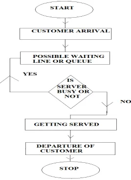
In general, a queue is formed at a queuing system when either customers ( human beings or
physical entities) requiring service wait due to number of customers exceeds the number of service
facilities or service facilities do not work efficiently and take more time than prescribed to serve a
customer. Hence “a group of items waiting to receive service, including those receiving the service is
known as a ‘waiting-line’ or a ‘queue’. The word ‘queue’ comes, via French, from the Latin ‘Canda’,
meaning ‘tail’ and is pronounced exactly like the letter ‘Q’.
The person waiting in a queue or receiving the service is called the ‘customer’ and the person
by whom, he is serviced is called a ‘server ‘.Point where service is provided is known as
‘service-station’. The idea about a queue may be expressed as under:
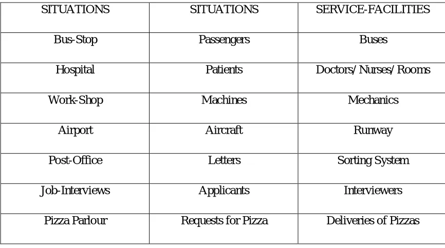
Some practical situations in which the solutions to waiting line problems can be find out using
queuing-theory are as under:
Table 1: practical situations
SITUATIONS SITUATIONS SERVICE-FACILITIES
Bus-Stop Passengers Buses
Hospital Patients Doctors/ Nurses/ Rooms
Work-Shop Machines Mechanics
Airport Aircraft Runway
Post-Office Letters Sorting System
Job-Interviews Applicants Interviewers
Pizza Parlour Requests for Pizza Deliveries of Pizzas
We have also seen that as a system gets congested, the service delay in the system increases.
A good understanding of relationship between congestion and delay is essential for designing
effective congestion control algorithms. Queuing theory provides all the tools needed for this
analysis.
COMMUNICATION DELAYS
:Before we proceed further, let’s understand the different components of delay in a messaging
system. The total delay experienced by messages can be classified into the following categories:
Processing Delay:
This is the delay between the times of receipt of a packet for transmission to the point of putting it
into the transmission queue.
On the receive end, it is the delay between the time of reception of a packet in the receive queue to
the point of actual processing of the message.
Queuing Delay:
This is the delay between the point of entry of a packet in the transmit queue to the actual point of
transmission of the message.
This delay depends on the load on the communication link.
Transmission Delay:
This is the delay between the transmissions of first bit of the packet to the transmission of the last bit.
This delay depends on the speed of the communication link.
Propagation Delay:
This is the delay between the point of transmission of the last bit of the packet to the point of
reception of the last bit of the packet at the other end.
This delay depends on the physical characteristics of the communication link.
Retransmission Delay:
This is the delay that results when a packet is lost and has to be retransmitted.
This delay depends on the error rate on the link and the protocol used for retransmissions.
In this paper we will be dealing with queuing delay. A queuing system is a birth-death
process with a population consisting of customers either waiting for service or currently in service. A
birth occurs when a customer arrives at the service facility; a death occurs when a customer departs
from the facility. Another factor that has an important effect on the behaviour of a queuing system is
the method that customers use to determine which line to join. For example, in some banks,
customers must join a single line, but in other banks, customers may choose the line they want to
join. When there are several lines, customers often join the shortest line. Unfortunately, in many
situations (such as a super market), it is difficult to define the shortest line.
CUSTOMERS BEHAVIOUR IN A QUEUE:
Customers generally behave in the following ways:
1. Balking: A customer may not like to wait in a queue due to lack of time or space or otherwise.
2. Reneging: A customer may leave the queue due to impatience.
3. Collusion: Some customers may collaborate and only one of them may join the queue. As at the
4. Jockeying: If there are more than one queue then one customer may leave one queue and join
the other. This occurs generally in the super market.
Hence if there are several lines at a queuing facility, it is important to know whether or not customers
are allowed to switch, or jockey, between lines. In most queuing systems with
multiple lines, jockeying is permitted, but jockeying at a toll booth plaza is not recommended.
IMPORTANT DEFINITIONS IN QUEUING PROBLEM:
Here we give the definitions of various terms used in the queuing theory.
1.
Queue Length: Queue length is defined by the number of persons (customers) waiting in
the line at any time.
2.
Average Length of Line: Average length of line (or queue) is defined by the number of
customers in the queue per unit time.
3.
Waiting Time: It is time up to which a unit has to wait in the queue before it is taken into
service.
4.
Servicing Time: The time taken for servicing of a unit is called its servicing time.
5.
Busy Period:
Busy-period for the server is the time during which he remains busy inservicing. Thus, it is the time between the start of service of the first unit to the end of
service of the last unit in the queue.
6.
Idle Period:
When all the units in the queue are served. The idle period of the server beginsand it continues up to the time of arrival of the unit (customer). The ideal period of a server is
the time during which he remains free because there is no customer present in the system.
7.
Mean Arrival Rate:
The mean arrival rate in a waiting-line situation is defined as theexpected number of arrivals occurring in a time interval of length unity.
8.
Mean Servicing Rate:
The mean servicing rate for a particular servicing station isdefined as the expected number of services completed in a time interval of length unity, given
that the servicing is going on throughout the entire time unit.
9.
Traffic Intensity:
In case of a simple queue the traffic intensity is the ratio of mean arrivalrate and the mean servicing rate.
We have developed some basic understanding of a queuing system. To further our understanding
we will have to dig deeps into characteristics of a queuing system that impact its performance. For
example, queuing requirements of a restaurant will depend upon factors like:
1. How do customers arrive in the restaurant? Are customer arrivals more during lunch and
dinner time (a regular restaurant)? Or is the customer traffic more uniformly distributed (a
cafe)?
2. How much time of customers spends in the restaurant? Do customers typically leave the
restaurant in a fixed amount of time? Does the customer service time vary with the type of
customer?
3. How many tables does the restaurant have for servicing customers?
The above three points correspond to the most important characteristics of a queuing system.
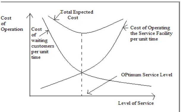
Obviously, an increase in the existing service facilities would reduce the customer’s waiting time.
Conversely, decreasing the level of service should result in long queue(s). This means an increase
(decrease) in the level of service increases (decreases) the cost of operating service facilities but
decreases (increases) the cost of waiting.
OBJECT OF THE QUEUING THEORY:
If there are queues then customers have to wait for some time before service. The time lost in
waiting is often expensive in terms of money, equipments, etc. As such there are costs associated
with waiting in line, commonly known as ‘waiting-time cost’. On the other hand, if there are no
queues, members of the servicing stations might stay idle and thus prove burdensome. Costs
associated with service or the facilities are known as ‘service cost’. The object of queuing theory is
to achieve a good economic balance between these two types of costs and the optimum solution is
arrived at a point where the sum of the waiting line and service costs is minimum. In brief, the object
of any queuing problems is to minimize the total waiting and service costs.
The above graph illustrates both types of costs as a function of level of service. Since cost of
waiting is difficult to estimate, it is usually measured in terms of loss of sales or goodwill when the
customer is a human being who has no sympathy with the service. But, if the customer is a machine
waiting for repair, then the cost of waiting is measured in terms of the cost of lost production.
It is important to note that queuing theory does not directly solve the problem of minimising
the total waiting and service costs but the theory provides the management with information
Figure 2: Types of costs as a Function of level of service
LITERATURE REVIEW:
Robert B. Cooper, Flouda Atlantic University, Shun – Chen Niu, University of Texas at
Dallas, Mandyam M. Srinivasan, University of Tennessee,1 In this paper they compared two versions
of a symmetric two – polling model. One of them is state – Independent setups, according to which
the server sets up at the polled queues whether or not work is waiting there. The other is State –
Dependent setups, according to which the server sets up only when work is waiting at the polled
queue. They find that the second version performs (i) the same as, (ii) worse than, or (iii) the better
than, its first version if the switchover and setup time, are respectively (i) both constants, (ii) variable
and constant or (iii) constant and variable.
The authors characterized the difference in the expected wating times of State – Independent setups
and State – Dependent setups through their paper.
Robert B. Cooper, Flouda Atlantic University, Shun – Chen Niu, University of Texas at
Dallas, Mandyam M. Srinivasan, In this paper the authors have tried to explain why the length –
biasing property of renewal theory is ubiquitous in queuing theory and why some recently –
uncovered surprising behaviour in polling models can be attributed its effects, using intuitive
The authors derived formulas that describe some results for polling models, such as the
reduction of waiting times as a consequence of forcing the server to set up even when no work is
waiting.
Consider the waiting time W in the ordinary M / G / 1 queue. The celebrated Pollaczek-Khintchine formula relates the mean waiting time to the basic parameters of the model (the arrival
rate λ of the Poisson arrival process, and the mean and variance of the service time S) as follows:
E(W) = ρ/(1 - ρ) ½ [E(S) + V(S)/E(S)] ...(1)
Where
ρ = λ E(S) if λ E(S) < 1, and, 1 if λ E(S) ≥ 1 ...(2)
and E and V denote the mean and variance, respectively.
The quantity ρ defined in (2) equals the utilization of the server. As (1) clearly shows, for any
positive value of ρ , no matter how small, E(W) can be arbitrarily large (because the variance-to-mean ratio V(S) / E(S), often called the “index of dispersion” in statistics, on the right- hand side of (1) can arbitrarily large). This is a truly remarkable and counterintuitive insight.
Furthermore, the probability that a customer will have to wait at all is P ( W > 0) = ρ (the
fraction of customers who find the server busy equals the fraction of time that the server is busy, by
PASTA; see Wolff), which is insensitive to the particular form of the service-time distribution
function. Thus, of two fundamental performance measures for M / G / 1, one of them (How often do
customers wait?) does not depend in any way on the variability of the service times, whereas the
other measure (How long do customers wait?) is quite sensitive to this variability.
The culprit here is, of course, the term
E(Y) = ½ [E(S) + V(S)/E(S)]= E(S2)/2V(S),
Robert B. Cooper, Shun – Chen Niu, Mandyam M. Srinivasan, In this paper the authors
developed simple implicit formulas for the expected waiting time as a function of mean and variance
of the setup times in standard polling models with either exhaustive or gated service discipline3.
Theorem 1 showed the expected waiting time can be reduced by inserting a forced idle time before
Theorem 1: If the service discipline is exhaustive, then
z*(k) = [1 – ρr] / [1 – ρk] √ gk , (1)
where gk is a constant given by
gk = V[Zk] + ∑ [Ґ(k ) / ρ12] V [ Zt]. (2)
The coefficients : { Ґ(k )i : 1 ≤ i ≤ N} in (2) are defined by
Ґ(k )t = ∑ [γ(k )jf ]2 , (3)
where (i) For k = 1, the constants { γ(k )tf : 1 ≤ i ≤ N; 0 ≤ c < ∞} are determined by the recursion
γjf (1) = [ρt / (1 – ρt )] [ ∑ γ(1 )jf + ∑ γ(1 )jf - 1 ] , (4)
with the initial condition γ(1 )jf - 1 = 1 and γ(1 )jf - 1 = 0 for 1 < i ≤ N - 1; and (ii) for 1 < k ≤ N, the
constants : { γ(k )tf : 1 ≤ i ≤ N; 0 ≤ c < ∞} are determined by the same recursion (4) after
renumbering the queues so that queue k becomes queue 1, queue k + 1 becomes queue 2, and so on.
In the special case of a symmetric polling model, the expected waiting time is given by the explicit
formula
E [W] = [ρT/ (1 – ρT)] [ b(2) / 2b] + (N / 2) (V [Z] / z) + (z / 2) [ (1 - ρT/ N) / (1 – ρT)] , (5)
and the minimizing value z*(k) = z* is the same for all queues, given by
z* = N √ [ V(Z) { (1 - ρT ) / (N - ρT ) }] (6)
R. B. Cooper, Shun – Chen Niu, Mandyam M. Srinivasan, In their paper, the authors
considered the classical polling model: queues served in cyclic order will either exhaustive or gated
service, each with its own distinct Poisson arrival stream, service - time distribution and switchover –
In my side the effect of these studies is to reduce computation and to improve theoretical
understanding of polling models.
Theorem 2: If the polling discipline is exhaustive service, then
E[ Wi ] = E[Wi0] + (R / 2) [(1 – ρi) / (1 – ρ)] (1)
Where Wi0 is the waiting time in the “corresponding” exhaustive – service model with zero
switchover times and correspondence parameters
xi(2) = bi(2) + δi-12 [ λi R / (1 – ρ)]-1 (2)
(2) If the polling discipline is gated service, then
E[ Wi ] = E[Wi0] + (R / 2) [(1 + ρi) / (1 – ρ)] (3)
Where Wi0 is the waiting time in the “corresponding” gated service model with zero switchover
times and correspondence parameters
xi(2) = bi(2) + δi2 [ λi R / (1 – ρ)]-1 (4)
The theorem says that in each case, the expected waiting time in the general-
switchover-times model equals the sum of the expected waiting time in the “corresponding” 0-swichover-switchover-times
model plus a simple term that depends only on the server utilization and the sum (but not the
individual values) of the mean switchover times.
In the important special case when the switchover times are (not necessarily equal) constants
(i. e., when δ2 = 0), then from (2) and (4), xi(2) = bi(2) and the “corresponding” 0-switchover-times model is the “true” corresponding 0-switchover-times model; that is, the effect of the switch-over
times is truly additive. During the course of our work, we learned via a preprint of Fuhrmann, that
this special case of the theorem was about to be published (and in fact, had been discovered in 1986).
Fuhrmann’s argument uses the concept of “ancestor” and “ancestral lines” in the same way as used
in Fuhrmann and Cooper (1985) in the analysis of decomposition in the M / G / I generalized-
vacations-model. Fuhrmann shows that, for constant switchover times, the population of customers
present in the system (represented by a vector whose components are the numbers of customers
present at each queue) at a poling epoch enjoys a stochastic decomposition. In contrast, our proof
(for the exhaustive- service case) begins with the vacation decomposition result itself, in its
mean-value form. Our argument, which is completely different from and independent of Fuhrmann’s, not
surprising generalization (for mean values) relative to Fuhrmann’s statement. That is, the
decomposition theorem retains its form even when the switchover times are random variables.5
M. M. Srinivasan, Shun – Chen Niu, R. B. Cooper, In this authors assumed, the queues are
attended by the server in cyclic order and they transformed results for the host of service disciplines
that completely characterized the relationship between the waiting times in these two polling models
with zero and non – zero switchover times6.
The authors established continuity in distribution of the waiting times and their transform
results can be used to drive, higher – moment generalization of expected – waiting times results.
Theorem 3: Under the exhaustive-service discipline, the LST of the waiting time in the
zero-switchover-times model is
W10(s) = [{λ (1 – ρ) / (1 – ρ1)} {H1( 1 – s / λ1) / s } ] W1*(s) (1)
Formula (1) which we believe is new, complements formula. The latter formula was derived based
on a Markov chain embedded at switch points, whereas ours is based on a Markov chain embedded
at polling epochs. It can be shown, via a proper “translation” between the solutions to these two
embedded chains, that these formulas are equivalent_
Shun – Chen Niu, R. B. Cooper, In this paper, authors analyzed to work with a modified
Markov Process that has a more detailed state description. At any time, when the server is busy, they
replace “the number of customers present” by two variables, (a) the number of customers who are
still waiting in the queue, and (b) the number of customers who arrived during that time service but
prior to that particular time. They show that this minor change of state definition makes possible a
surprisingly simple analysis of the M / G / I / K queue. In this paper the authors work with the
Poisson – arrival case because of its simplicity and its basic importance7.
In my opinion, the basic method already has been explained here, and they are focusing on the
computational issues.
S. W. Fuhrmann, AT & T bell Laboratories, Holmdel, New Jersey, R. B. Cooper, In this
paper authors considered a class of M / G / I queuing models with a server who is unavailable for
occasional intervals of time. The times when the server is unavailable may correspond to times when
as the sum of two or more independent random variables, holds, in fact, for a very general class of M
/ G / I queuing models8.
The M / G / I decomposition property holds for all M / G / I models of general form. In my opinion
the parallel decomposition of waiting times was demonstrated in a more confined manner.
R. B. Cooper, [1976], In this paper, the author considered a queuing system in equilibrium in
which arrive according to a Poisson process and request service from a group of parallel
heterogeneous exponential servers. The strategy of this paper is to attack the problem of ordered
heterogeneous servers through application of some ideas that tale traffic theorists have used in
studies of ordered homogeneous servers. This approach permits solution of the problems of ordered
heterogeneous servers without necessitating the solution of the detailed multidimensional birth and
death equations9.
If the servers are homogeneous, the order of search for an idle server is irrelevant unless one is
interested in the behavior or states of a particular server instead of only the behavior of the system as
a whole.
R. B. Cooper, In this paper, the author extends previous study of cyclic queues to obtain
waiting time results, for both the exhaustive service model and the gating model. In this paper, the
Laplace – Stieltjes transforms of the order – of - arrival waiting time distribution functions and for
the exhaustive service model, the mean waiting time for a unit arriving at a queue, are obtained9.
In the present paper, we obtain the desired waiting time results without recourse to a
complicated reformulation of the original analysis based on the complete set of service completion
points. Rather, to obtain the waiting times at queue i, we use the generating function gi-1 (x1, ...xN),
to append to the original set of switch points only those service completion points that correspond to
departure from queue i; and this is sufficient for our waiting time calculations.
The essence of the method is to calculate the probability generating function of the number of
units left in queue i by an arbitrary departure from queue i, using only the (known) probability generating function of the number of units waiting in the queue i when the server arrives. The Laplace-Stieltjes transform of the order – of –arrival waiting time distribution function for units at
queue i is then easily obtained by a standard argument.
The preceding discussion refers mainly to the exhaustive service model, which was discussed
those of the exhaustive service model, and was therefore not developed in details. In the present
paper, the waiting times for gating model will also be discussed.
R. B. Cooper, and G. Murray*(* The RAND Corporate), In this paper, the authors studied the
two models of queues served in cyclic order by a single server, the exhaustive service model and the
gating model. The authors found expression for the mean number of units in a queue at the instant it
starts service, the mean cycle time, and the Laplace – Stieltjes transform of the cycle time
distribution function10.
The authors showed that the gating model is described by state equations only trivially different from
those of the exhaustive service model. In my opinion, now it is easy to modify the methods and
results of the detailed analysis of both models.
COMPUTING ALGORITHM
The following computing algorithm has been developed to compute the optimal service rates
and total optimal cost and profit of the system with two priority classes.
Step 1: begin
Step 2: input all variables
Step 3: compute derived variables
Step 4: compute derivatives
Step 5: compute functions
Step 6: t1 ← initial service rate of HPC
Step 7: t2 ← initial service rate of LPC
Step 8: iterating initial service rates
Step 9: while (error=0.0000000001)
Step 10: compute optimal service rates
Step 11: compute total optimal cost
NUMERICAL DEMONSTRATION OF THE RESULTS
Numerical demonstration is very useful to exhibit the results (performance measures) of the
model. It focuses on the sensitivity analysis of one parameter relative to other parameters for
determining the direction of future data-input. Parameters for which the model is relatively sensitive
would require more attention of researchers engaged in this field, as compared to the parameters for
which the model is relatively insensitive or less sensitive.
S. S. Mishra and D. K. Yadav, The paper focused on cost and profit analysis of single –
server Markovian queuing system with two priority classes. In this paper, functions of total expected
cost, revenue and profit of the system are constructed and subjected to optimization with respect to
its service rates of lower and higher priority classes. A computing algorithm is also developed, by the
authors, to solve the system of non linear equations formed out of the mathematical analysis.
In this paper the evaluation of total expected profit of both priority classes and of whole
system has been carried out. In my opinion, it brings the power to produce the desired effect of the
model close to a realistic situation11.
G. Vijya Lakshmi, C. Shoba Bindu, Dept. of CSE, JNTUA College of Engineering, Anantpur
– 515001, India, In this paper the author designed a access network which is congestion free and it is
also observed that by the help of queuing model, a best traffic is achieved. Good scheduling,
reliability and congestion free environment is been observed on static as well as random networks12.
With economic constraints and limited routing capability, the structure of an access network
is a challenging design. In my opinion it is also important to prevent access network especially as
voice, video and data traffic for survivability.
Sangeeta Agarwal, K R Subramaniam & S. Kapoor, This paper is authors attempted to study
the importance of operation research and various techniques used to improve the operational
efficiency of the organization. According to authors, organization leaders can make high quality
decisions. Only if, he or she must have fundamental knowledge of tools and acquire right
resources13.
S. S. Mishra (The Dept. of Maths & Statistics, Dr. Ram Manohar Lohia Avadh University,
Faizabad, U. P., India), In this paper the author computed the total optimal cost of interdependent
queuing system with controllable arrival rates. A numerical demonstration based on computing
algorithm and variational effects of the model with the help of the graph have also been presented by
VARIATIONAL ANALYSIS:
Validity of any model depends on the variation-effect of one parameter on the other
parameters involved therein. Here, different types of analyses are being given in fig. 1.as:
- Cost per Unit Service Rate Vs Total Optimal Cost.
-Holding Cost Vs Total Optimal Cost.
- Initial Arrival Rate Vs Total Optimal Cost.
- Reduced Arrival Rate Vs Total Optimal Cost.
Finally, we conclude with the remark that present research on optimum performance
measures of the interdependent queuing model with controllable arrival rates can pave the way for
future progress of research in various fields including technical applications for the digital
communication systems and as well as in assessing the performance measures in the form of optimal
service and cost of computer networking by applying this queuing approach. Such systems are often
encountered in practice, particularly in service-oriented operations, which brings the efficacy of the
model closer to a realistic situation. The aim of the numerical demonstration is to study the
variability of the model that is, to assess the effect of one parameter on the others especially such
parameters which characterize the performance measures of the model. Numerical demonstration
carried out with the help of search program is mainly based on the simulations or hypothetical
data-input. In this paper, we have preferred the hypothetical data-input to run the search program
developed in the paper, which at later stage can also be tested for any real case study. It has also a
good deal of potential to the applications in other areas such as inventory management, production
management, computer system etc.
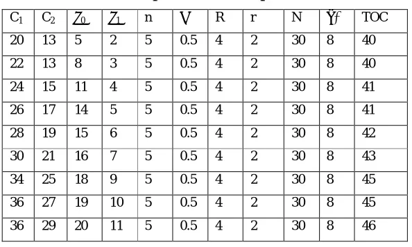
Table 2:Computation of Total Optimum Cost
C1 C2 λ0 λ1 n ε R r N μ* TOC
20 13 5 2 5 0.5 4 2 30 8 40
22 13 8 3 5 0.5 4 2 30 8 40
24 15 11 4 5 0.5 4 2 30 8 41
26 17 14 5 5 0.5 4 2 30 8 41
28 19 15 6 5 0.5 4 2 30 8 42
30 21 16 7 5 0.5 4 2 30 8 43
34 25 18 9 5 0.5 4 2 30 8 45
36 27 19 10 5 0.5 4 2 30 8 45
Fig.3. Graphic representation of Total Optimum Cost
Ibtissam Hdhiri and Monia Karouf, In this paper the authors considered the problem of an
optimal stochastic impulse control of non – Markovian Processes when the expression of the cost
functional integers sensitiveness with respect to the risk. They try to establish the existence of an
optimal strategy. They prove that impulse control problem could be reduced to an iterative sequence
of optimal stopping ones15.
Theorem 4: The strategy δ* is optimal and (Y)t ≤ T is the value function of the risk - sensitive
impulse control problem, i.e., for any t ≤ T we have :
Yt(0, 0) = ess sup E[exp { ∫ h ( s, w, Lsδ ) ds - ∑ ψ ( ξn ) Ц [_Tn < T] }Ft] ,at δ Є D (6)
In particular, Y0(0, 0) = sup J(δ) = J(δ*) , at δ Є D
Proofs:
*Thanks to the last proposition Y( υ, ξ) is a cadlag process
*continuity
-- Yt( υ, ξ) exp{∫ h ( s, Ls+ ξ ) Ц [_s ≥υ] ds}) is a Snell envelope of
(exp{∫ h ( s, Ls+ ξ ) Ц [_s ≥υ] ds} Oi ( υ, ξ) 0 ≤ i≤ T
-- Doob-Meyer decomposition implies that:
Yt( υ, ξ) exp{∫ h ( s, Ls+ ξ ) = Mt - At – Bt ; t ≤ T:
-- ∆Bt = - ∆Yt.
YT ( υ, ξ) < YT -( υ, ξ) = exp(-ψ(β0)) Ц [_Tn < T] YT -( υ, ξ + β0)
Then there exists another r.v β1Є U such that:
∆tY (υ, ξ + β1) < 0 and YT -( υ, ξ) = exp((-ψ(β1)) Ц [_Tn < T] YT -( υ, ξ + β1)
...
...
YT - ( υ, ξ) < exp(-nc + γT)
-- The strategy δ* = (τn*, βn* ) n > 0Є D and it is optimal.
Muhammed El - Taha, Dept. of Mathematics and Statistics, University of Southern Main 96,
Falmouth Street, Portland, U. S. A.16
Theorem 5:Consider the G/G/1 stable multi-class multiple vacation model with WCS rules that are
non-preemptive, regenerative, and within each class, they are service time independent. Also,
suppose and, and that for each and are asymptotically path wise uncorrelated. The vector of expected
actual queue delays per customer satisfies the conservation law.
This theorem can be used to construct conservation laws for waiting time in the system, number of
customers in the system, and number of customers in the queue using the fact that and Little's
formula. In this paper, we give two primary results. The first result is “Consider the G/G/1-FIFO
multi vacation model. Suppose that and, and that and are asymptotically path wise uncorrelated”,
gives a relation between virtual delay and actual delay for single-server multiple vacation model
under conditions that are weaker than those given in the literature. This result is extended to
multi-class models where a conservation law is “Consider the G/G/1 stable multi-multi-class multiple vacation
model with WCS rules that are non-preemptive, regenerative, and within each class, they are service
time independent. Also, suppose and, and that for each and are asymptotically path wise
uncorrelated. The vector of expected actual queue delays per customer satisfies the conservation
law”, which is our second result. We use sample path analysis which allows us to give rigorous
arguments by focusing on one realization of the stochastic process that describes the system
CONCLUSION:
Really operations research techniques right from inception during World War II are of great
use for optimum allocation of limited resources. Queuing theory is to distribute service or resources
to prospective users. Authors of this paper collected and analyzed the techniques by researchers and
have given model to develop further techniques in managing queues.
REFERENCES:
1. Robert B. Cooper, Flouda Atlantic University, Shun – Chen Niu, University of Texas at Dallas, Mandyam M. Srinivasan, University of Tennessee,: “Setups in Polling Models: Does it make sense to set up, if no work is waiting?” Journal of Applied Probability, printed in Israel. © Applied Probability Trust, 1999; 36: 585 – 592, 1999.
2. Robert B. Cooper, Flouda Atlantic University, Shun – Chen Niu, University of Texas at Dallas, Mandyam M. Srinivasan, “Some Reflections on the Renewal – Theory Paradox in Queueing Theory” Journal of Applied Mathematics and Stochastic Analysis (J. A. M. S. A. ), Special Issue Dedicated to RYSZARD SYSRI, North Atlantic Science Publishing Company {USA}. 1998:11(3): 355 – 368.
3. Robert B. Cooper, Shun – Chen Niu, Mandyam M. Srinivasan, August, “When Does Forced Idle Time Improve Performance in Polling Models?”, Management Science, 1998; 44(8): 1079 – 1086.
4. R. B. Cooper, Shun – Chen Niu, Mandyam M. Srinivasan. “A Decomposition Theorem for Polling Models: Theswitchover Times are Effectively Additive”, Operations Research, 1996; 44(4): 629 – 633.
5. S. W. Fuhrmann, AT & T bell Laboratories, Holmdel, New Jersey, R. B. Cooper. “Stochastic Decompositions in the M / G / I Queue with Generalized Vacations”, Operations Research, 1985; 33(5): 1117 – 1129.
6. M. M. Srinivasan, Shun – Chen Niu, R. B. Cooper, “Relating Polling Models with Zero and
Non – Zero Switchover Times”, Queuing System [November 09, 1993, Revised: March 29,
1994, August 12, 1994]: 1995; 19: 149 – 168.
7. Shun – Chen Niu, R. B. Cooper, “Transform – Free Analysis of M / G / I / K and Related Queues”, Mathematics of Operations Research, Printed in USA, 1993; 18(2): 486 – 510.
8. R. B. Cooper, “Queues with Ordered Servers that Work at Different Rates”, Operations Research, 1976; 13(2): 69 – 78.
10. R. B. Cooper, and G. Murray*(* The RAND Corporate),: “Queues Served in Cyclic Order”, The Bell System Technical Journal, 1969; 48(3): 675 – 689
11. S. S. Mishra and D. K. Yadav. “Cost and Profit Analysis of Markovian Queuing System with Two Priority Classes: A Computational Approach”, International Journal of Mathematical and Computer Sciences. 2009; 5(3): 150 – 156.
12. G. Vijya Lakshmi, C. Shoba Bindu, Dept. of CSE, JNTUA College of Engineering, Anantpur – 515001, India, “A Queuing Model for Congestion Control and Roliable Data Transfer in Cable Access Networks”, International Journal of Computer Science and Information Technologies (1J, CSIT), 2011; 2(4): 1427 – 1433.
13. S. S. Mishra (The Dept. of Maths & Statistics, Dr. Ram Manohar Lohia Avadh University, Faizabad, U. P., India), “Optimum Performance Measures of Interdependent Queuing System with Controllable Arrival Rates”, World Academy of Science, Engineering and Technology 2009; 57: 820 – 823.
14. Sangeeta Agarwal, K R Subramaniam & S. Kapoor. “Operations Research – Contemperary
Role in Managerial Decision Making”, IJRRAS. 2010; 3 (2): 200 – 208.
15. Ibtissam Hdhiri and Monia Karouf. “Risk Sensitive Impulse Control of Non – Markovian Process”, Mathematical Methods of Operations Research, 2011; 74: 1 – 20.