Homotopy Classes and Cell Decomposition
Algorithm to Path Planning for Mobile
Robot Navigation
Mahmoud Wahdan
1, Mohamed. M.Elgazzar
21
Faculty of Information Systems & Computer Sciences, 6 October University , Giza, Egypt
2Ass.Prof., Higher institute of Computer Sciences and Information systems fifth Settlement, NewCairo, Egypt
Abstract- This paper describes an algorithm of homotopy classes and cell decomposition to path planning for robot motion planning. The motion planning problem of a rigid body vehicle is divided into two subproblems in this method: (i) decomposing a given free space into a finite number of simple shaped regions in such a way that the second subproblem become natural and easy, and (ii) planning a detailed motion from the start position/orientation to the goal using the aforementioned global path. This paper mainly deals with the first subproblem. In this method, the most important point is how to decompose a world into simpler regions called cells. The method proposes several new concepts including fences. The planned path is a sequence of fence sequence belonging to these cells. In this paper, we propose homotopy classes and cell decomposition as a solution to subproblem (i). Probably, this decomposition method is the first method proposed for symbolic representation of homotopy classes.
I. INTRODUCTION
The motion planning problem for a robot is not a simple task. It is advantageous to divide a complex problem into subproblems. This problem can be divided into the following two distinct subproblems:
1. global path planning, and 2. local motion planning.
where the global path planning task is to decide the best path class and the local motion planning task is to determine the exact motion. This paper discusses several aspects in the first issue. The discussions and analyses given in this paper is related to the most abstract level of all path/motion planning problems, since only the connectivity of geometrical objects are discussed.
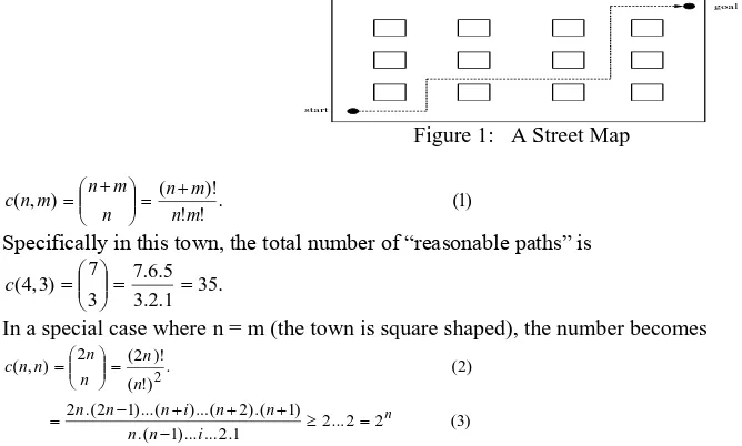
Let us consider a town which has n+1 streets and m+1 avenues with n, m 1. Namely, this town consists of mn counterclockwise (ccw) polygons and one cw polygon. An example is shown in Figure 1 where n = 4 and m = 3. Now consider paths from the SW corner to the NE corner consisting of only north bound or east bound segments. How many distinct paths generally exist? Notice that the path shown in the Figure can be symbolically described as “ENEENNE”. The number of distinct paths is equal to the number of combinations of taking n eastbound segments out of all n + m segments. Therefore, the total number c(n, m) of combinations is
start
goal
Figure 1: A Street Map
) 1 ( . ! ! )! ( ) , ( m n m n n m n m n
c
Specifically in this town, the total number of “reasonable paths” is
. 35 1 . 2 . 3 5 . 6 . 7 3 7 ) 3 , 4 ( c
In a special case where n = m (the town is square shaped), the number becomes
and this function c is not polynomial of n. That means if we execute an exhaustive search, the computation cost is extremely high. Notice that if we allow southbound or westbound segments, i.e. we allow cycles, there are infinitely many distinct paths.
In this paper, we propose Homotopy classes and cell decompositions as a solution to unambiguous symbolic representation of Homotopy classes. The meaning of “optimality” is not addressed in this paper. We propose a general framework under which the motion planning problem is effectively solved with an arbitrary cost function for optimality.
Previously several cell decomposition methods have been proposed [1, 2, 3, 4]. Vertical and horizontal decompositions by Chazelle [2] are special ones of convex decompositions. The concept of convex decompositions is used instead of vertical or horizontal decomposition for a given polygonal world [5].
Several concepts and theories have been developed which may lead to solve the motion planning problem. The configuration space approach is one global motion planning method using the concept of the vehicle configuration (x, y, ) [6]. The artificial potential field method is a path planning method for a point robot. [7]. The Voronoi diagrams method is one of a robot path planning [8]. Other class of path planning methods based on Voronoi diagram which can be implemented either as off-line algorithm [9] or on-line algorithm [10]. In Voronoi diagram based algorithms the resultant path consists of line segments which make the robot stop at each line segment, change its direction and continue. Such movement causes power consumption to the robot. In order to overcome this problem and satisfy initial position and shortest path conditions two Bezier curves are used [11, 12].
There are a lot of algorithms to find a collision-free path [13, 14]. Most of them are based on the so called road map approaches like visibility graph method.
Different obstacle avoidance path planning approaches have been reported in the literature [15] [16], including ones using potential fields [17] [18].
One commonly used approach is based on the Dijkstra’s algorithm, finding the shortest path through a graph representing an environment [19].
The other global motion planning ideas can be found in other research reports. Some of these focuses on the motion planning for manipulators [20] and others provide general ideas [21, 22, 23, 24, 25, 26].
II. HOMOTOPY
We consider a plan 2 with holes. A hole is an obstacle for a robot, which is a point in this section. A free space F is the complement of the union of all holes. There might be a hole among them which completely surrounds the free space, which is said to be inverted. Every free space is a connected subset of 2 (Fig. 2).
(a) Without inverted hole (b) With inverted hole Figure 2: Worlds with Holes
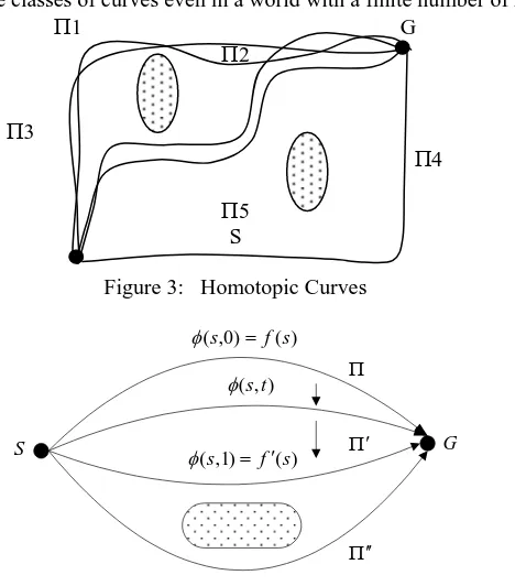
In this section, a directed curve or a directed path is represented by a continuous function f: [0, 1] F. The two points f (0) and f (1) are called its endpoints of . The curve is said to join the endpoints. A curve has its natural direction from f (0) to f (1). Obviously, there are infinitely many curves joining given two points S and G in F (Fig. 3). In this Figure, curves 1 and 2 are somewhat similar and so are curves 3 and 4. However, 1 and 3 are not. This concept has formally defined in the field of algebraic topology [27] and will be followed. Two curves and (defined by f and f respectively) are said to be homotopic if and only if there exists a continuous function : [0, 1] x [0, 1] F such that
(0, t) = f (0) for all t [0, 1],
(1, t) = f (1) for all t [0, 1],
(s, 0) = f (s) for all s [0, 1], and
i.e., informally speaking, can be continuously transformed into without running over any holes with both endpoint fixed (Fig. 4). If and are equivalent, we write
(4)
Obviously, this relation depends on the free space F and their endpoints. In Figure 3, 1 2 and 3 4. Proposition 1 2 The relation is an equivalence relation [27].
There are countable equivalence classes of curves even in a world with a finite number of holes.
1 G
2
3
4
5 S
Figure 3: Homotopic Curves
) ( ) 0 , (s f s
) , (st
) ( ) 1 , (s fs
S G
Figure 4: Continuous Transformation of Curves
III. REPRESENTATION OF HOMOTOPY CLASSES
Now we consider the problem of “how to symbolically represent each Homotopy class in a given F?”. We present a method based on “fences” in this paper.
We assume that a world contains a finite number n of a normal hole. If an inverted hole does not exist in the world, we consider an imaginary inverted hole enclosing all the normal holes with an indefinitely large size. A fence L in this world is a loop-free curve which connects two holes, where L does not intersects any holes except at its endpoints. We add n fences to the world in a way such that all the n + 1 holes are connected. A structure consisting of n + 1 holes and n fences is said to be a connected world (Fig. 5). Obviously, for a world with n 2, there are more than one way to construct connected world.
Figure 5: Connected World (I)
Proposition 2 In a connected world,
There exists no cycle that is made by holes and fences.
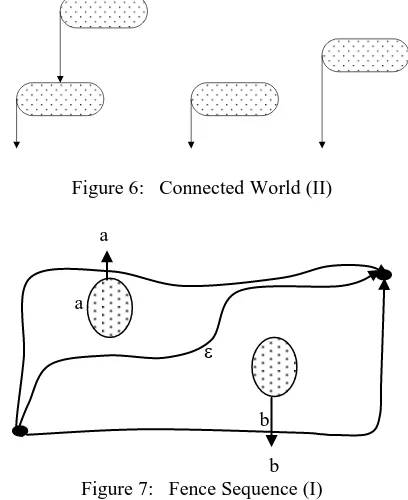
One “standard” way to connect a world by fence is to add vertical downward fences at the left end of each holes (Fig. 6).
In a three-hole world shown in Figure 7, three distinct Homotopy classes can be represented by fences which are crossed by paths: , a, b
Figure 6: Connected World (II)
a
a
b
b Figure 7: Fence Sequence (I)
If we consider some other classes of paths, however, it is better we give an orientation to each fence. We redefine a fence so that it has two sides: a plus side and minus side (Fig. 8).
-a
-+
+
b
a
b a b
S
G
Figure 8: Fence Sequence (II)
A curve (represented by f) is said to intersect a fence L if there exists an s [0, 1] such that f (s) is on L and two points f (s + ), f (s - ) are on the opposite sides of L if > 0 is small enough. We differentiate the two types of intersecting relations of a path and a fence L. If the path intersects L from its plus side to its minus side, its intersecting mode is said to be the plus mode and is expressed by a symbol L+; otherwise, it is said to be minus mode and is expressed by a symbol L-. If a world has a finite number of fences, the set of all intersecting modes is
= { L+, L- L is a fence in the world}. (5)
If a fence sequence fs() has a subsequence of a form L+ L- or L- L+ (Fig. 9(a)), a part of the curve can be simplified, because
Proposition 3 For a curve , if there exist a fence L and fence sequence 1, 2 such that
fs() = 1 L+ L- 2 (6)
fs() = 1 L- L+ 2 (7)
there exists a curve such that and
A curve is said to osculate a fence L if there exists an s [0, 1] such that f(s) is on L and two points f(s + ), f(s -
) are on the same side of L if > 0 is small enough (Fig. 9(b)). We can eliminate the portion, because
L
-+
L
-+
L
L
(a) Complementary modes (b) Osculating curve Figure 9: Pathological Fence Sequences
Proposition 4 If a curve is osculating a fence L in a connected world, there exists a curve such that and
does not osculate L.
Proof. Obtain by replacing the part from f(s + ) to f(s - ) by a sub-curve which does not osculate or intersect with L.
By these Propositions, we hereafter assume that, for any curve , its fs() does not contain L+ L- or L- L+ for some L, and
does not osculate any fence.
Now we prove that fs() is necessary and sufficient to represent its path class.
Lemma 1 Let S, T be points (possibly the same) in the free space of a connected world. If fs() = fs() = for two curves and , .
Proposition 5 For any curves and , if fs() = fs(), . Proof. We transform into part by part.
We proved the half of the fact we wanted to prove. Proposition 6 For any curves and , if , fs() = fs().
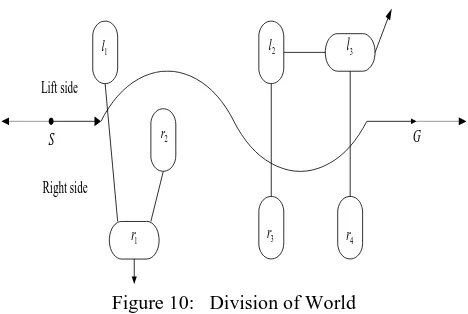
Sketch of the Proof. First consider the case where no fence L occurs in fs() more than once. Let us draw fences LS and LG from S and G to the inverted hole (Fig. 10). Then the structure of the inverted hole, , LS, and LG divide the whole world into two sides. Then each normal hole belongs either side. No continuous change of does not change this division of holes. Therefore, each intersection with a fence does not disappear nor newly generated. If the same L appears in fs() more than one time, we divide into several parts and develop a similar discussion as stated above.
1
l l2 l3
1
r
2
r
3
r r4
S G
Lift side
Right side
Figure 10: Division of World
IV. CELL DECOMPOSITION AND CONNECTIVITY GRAPH
In this Section, we assume all example worlds are rectilinear. Although all the discussions in this Section are workable to general worlds with minor changes, this assumption makes some part of the discussions easier. Furthermore, at this moment, we assume that all holes are rectangles.
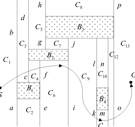
Consider a vertical tangents to a hole in a world. If a hole is convex, there are two vertical tangents (Fig. 11). A vertical tangents is divided into two vertical fences. Therefore, in this method, we generate four fences for each hole (remember that, as Fig. 6 shows, we used only one fence to each hole in the previous Section). The purpose of adding more fences is not only to specify distinct path classes, but also to divide the free area F into smaller subareas with simpler shapes. Each area generated by fences and hole boundaries is called a cell (Fig. 12). In this Section, a fence means one half of a vertical tangent defined above.
Hole
fence
fence
vertical tangent
Figure 11: Vertical Tangents
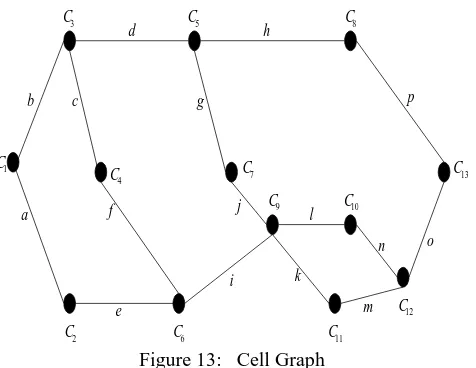
This cell decomposition defines a graph whose nodes are areas and whose edges are fences. The graph generated by the world in Figure 12 is shown in Figure 13. With this graph, we can include all geometrical information to help the detailed navigation task. Thus some portion of the motion planning problem is converted to a straightforward graph search problem.
Construction of cell decomposition and cell graph can be done as preprocessing for a motion planning system. We propose that both vertical and horizontal decomposition are constructed in the preprocessing stage and a user uses either one when a pair of S and G is given.
3
B
1
B
2
B
4
B
b
a
e
i
o
m
k
n
l
j
g
d
h
p
f
c
S
G
1C
2
C
3C
4
C
5
C
6
C
7
C
8
C
9
C
C
1011
C
12
C
13
C
1 C
2 C 3 C
4 C
5 C
6 C
7 C
8 C
9
C C10
11 C
12 C
13 C
a
b c
d h
p g
j f
e
i k
l
m
n o
Figure 13: Cell Graph
Lemma 2
Each cell generated by fences has one of the following shapes. (a) an orthogonal rectangle, (b) an area bounded by three orthogonal edges, or (c) an area bounded by one vertical line. These areas are said to be generalized rectangles. When we have n normal holes in a world and their positioning is general, there are 3n + 1 cells generated by vertical tangents.
Now we can represent a path class by its fence sequence as shown in Figure 12. The fence sequence of the path shown in the figure is bcfikmo. If we specify the cells as well as fences,
C1 b C3 c C4 f C6 i C9 k C11 m C12 o C13 (9)
Lemma 2 In this cell decomposition method, we do not need to specify the orientation of each fence.
We say a path is loop-free if it does not visit the same cell twice. In realistic situations, we are only interested in loop-free paths and loop-free path classes.
An advantage of this method is the second “detailed motion planning” problem becomes simpler if a fence sequence in cell decomposition is given.
V. THE SEARCH ALGORITHM
The purpose of the SEARCH algorithm is to generate all distinct path classes between two identified nodes. To accomplish this task the depth first search is adopted in the algorithm.
The input of the initial routine GEN_PATH_CLASS() are G, the cell graph, s, the node which represents the cell containing start configuration and g, the node which represents the cell containing goal configuration.
The outputs of the algorithm are all distinct path classes represented by fence sequences and the number of path classes if start and goal configurations are not in the same cell. Otherwise, print the message "The start and goal configurations are in the same cell".
The algorithm can now be described as follows:
ALGORITHM PATH CLASSES METHOD GEN_PATH_CLASS (G, s, g)
if s = g
output ("the start and goal configurations are in the same cell")
else
for each node v in V [G] parent [v] = NIL count = 0
parent [s] = s DFS_VISIT (G, s, g) output (count)
if u = g
count = count + 1 PRINT_PATH else
for each node v adjacent to u if parent [v] = NIL parent [v] = u DFS_VISIT (G, v, g) parent [v] = NIL
Applying this algorithm to Figure 13, there are 12 simple paths from S to G represented by fence sequences. A simple path is a path which visits a cell at most once. The following are the listing of these paths:
1. b d h p 2. b d g j l n o 3. b d g j k m o 4. b c f i l n o 5. b c f i k m o 6. b c f i j g h p 7. a e i l n o 8. a e i k m o 9. a e i j g h p 10. a e f c d h p 11. a e f c d g j l n o 12. a e f c d g j k m o
VI. CONCLUSIONS
The proposed homotopy classes and cell decomposition method gives a new solution to the path planning problem. This method gives answers to the following: how to symbolically represent homotopy classes? and how to find the “optimal” path class for a given pair of robot configurations. The results are:
The set of “fence sequences” in a “homotopically decomposed world” is an answer to first question. The “connectivity graph” of a homotopically decomposed world is an answer to second question.
An advantage of this method is the second “detailed motion planning” problem becomes simpler if a fence sequence in cell decomposition is given.
VII. REFERENCES
[1] R. A. Brooks and T. Lozano-Perez. A Subdivision Algorithm in Configuration Space for FindPath with Rotation. Proceedings of the 8th International Conference on Artificial Intelligence, Karlsruhe, FRG, pp. 799-806, 1983.
[2] B. Chazelle. Approximation and Decomposition of Shapes. In [Schwartz and Yap, 1987], pp. 145-185.
[3] G. E. Collins. Quantifier Elimination for Real Closed Fields by Cylindrical Algebraic Decomposition. Lecture Notes in Computer Science, 33, Springer-Verlag, New York, pp. 135-183, 1975.
[4] A. Lingas. The Power of Non-Rectilinear Holes. Proceedings of the 9th Colloquium on Automata, Languages and Programming, Arhus LNCS Springer-Verlag, pp. 369-383, 1982.
[5] M. Wahdan, Theory of path classes for robot motion planning using area decomposition. The 36th Annual Conference on Statistics, Computer Science and Operation Research, Cairo, Dec. 2001
[6] T. Lozano-Perez. Special Planning: A Configuration Space Approach. IEEE Transaction on Computers, vol. C-32, no. 2, pp. 108-119, Feb. 1983.
[7] G. Li, Y. Tamura, A. Yamash and H. Asama. Effective improved artificial potential field-based regression search method for autonomous mobile robot path planning. Int. J. Mechatronics and Automation, vol. 3, no. 3, 2013.
[8] J. Canny and B. Donald. Simplified Voronoi Diagrams. Springer-Verlag, pp. 272-289, 1987.
[9] P. Bhattacharya and M. L. Gavrilova. Voronoi diagram in optimal path planning. 4th International Symposium on Voronoi Diagrams in Science and Engineering (ISVD 2007).
[10] S. Mohammadi and N. Hazar. A Voronoi-Based Reactive Approach for Mobile Robot Navigation. H. Sarbazi-Azad et al. (Eds.): CSICC 2008, CCIS 6, pp. 901–904, 2008.
[11] A. Sahraei1, M. T. Manzuri, M. Tajfard and S. Khoshbakht. Obstacle Avoidance using a Near Optimal Trajectory for Omni-directional Mobile Robots. 12th International CSI Computer Conference (CSICC'07) Shahid Beheshti University, Tehran, Iran, 2007.
[12] J.W. Choi, R.E. Curry and G.H. Elkaim. Real-time obstacle avoiding path planning for mobile robots. In: Proceedings of the AIAA Guidance, Navigation and Control Conference, AIAA GNC 2010, Toronto, Ontario, Canada, 2010.
[13] J Lotombe and J. Claude. Robot motion planning. Kluwer Academic Publisher.
[15] J.K. Goyal and K.S. Nagla. A new approach of path planning for mobile robots. In Advances in Computing, Communications and Informatics (ICACCI, 2014 International Conference on, pp.863-867, 24-27 Sept. 2014.
[16] C. Keonyup, L. Minchae and S. Myoungho. Local Path Planning for Off-Road Autonomous Driving With Avoidance of Static Obstacles. In Intelligent Transportation Systems, IEEE Transactions on, vol.13, no.4, pp.1599-1616, Dec. 2012.
[17] T. Lei, D. Songyi, G. Gangxu, Z. Kunli, W. Suihe, and F. Xinghuan. A novel potential field method for obstacle avoidance and path planning of mobile robot. In Computer Science and Information Technology (ICCSIT), 2010 3rd IEEE International Conference on, vol.9, pp. 633-637, 9-11 July 2010.
[18] Keonyup, C.; Minchae, L.; Myoungho, S., ”Local Path Planning for Off-Road Autonomous Driving With Avoidance of Static Obstacles,” in Intelligent Transportation Systems, IEEE Transactions on , vol.13, no.4, pp.1599-1616, Dec. 2012.
[19] Lei, T.; Songyi, D.; Gangxu, G.; Kunli, Z.; Suihe, W.; Xinghuan, F., ”A novel potential field method for obstacle avoidance and path planning of mobile robot,” in Computer Science and Information Technology (ICCSIT), 2010 3rd IEEE International Conference on , vol.9, pp.633-637, 9-11 July 2010.
[20] Z. Li and L. Wei. Adaptive Artificial Potential Field Approach for Obstacle Avoidance Path Planning. In Computational Intelligence and Design (ISCID), 2014 Seventh International Symposium on, vol.2, no., pp. 429-432, 13-14 Dec. 2014.
[21] Yi, Y.; Guan, Y., ”A Path Planning Method to Robot Soccer Based on Dijkstra Algorithm,” in Advances in Electronic Commerce, Web Application and Communication, vol. 2, pp.89-95, 2012
[22] Y. Yi and Y. Guan. A Path Planning Method to Robot Soccer Based on Dijkstra Algorithm. In Advances in Electronic Commerce, Web Application and Communication, vol. 2, pp. 89-95, 2012.
[23] Y. K. Hwang, P. C. Chen, A. A. Maciejewski, and D. D. Neidigk. A Global Motion Planner for Curve-Tracing Robots. IEEE int. Conf. on Robotics and Automation, pp: 2-7, 1994.
[24] T. Fraichard and C. Laugier. Path-velocity Decomposition Revisited and Applied by Dynamics Trajectory Planning. IEEE int. Conf. on Robotics and Automation, pp: 40-45, 1993.
[25] Y. K. Hwang and N. Ahuja. Gross Motion Planning – A Survey. ACM Computing Surveys, Surv., 24(3), pp: 219-291, 1992. [26] F. H. Croom. Basic Concepts of Algebraic Topology. Springer-Verlag, 1978.
[27] A. Antti and L. Johannes. Robot motion planning by a hierarchical search on a modified discretized configuration space. IEEE International Conference on Intelligent Robots and Systems. vol. 2, pp: 1208-1213, 1997.
[28] J. Sharifi and W. WJ. Fast approach for robot motion planning. Journal of Intelligent and Robotic Systems:-Theory-and-Applications. Vol: 25, pp: 187-212, 1999.