e-ISSN: 2278-067X, p-ISSN: 2278-800X, www.ijerd.com
Volume 11, Issue 07 (July 2015), PP.01-07
Single Hard Fault Detection in Linear Analog Circuits Based On
Simulation before Testing Approach
G.Puvaneswari
1, S.UmaMaheswari
21Department of Electronics and Communication Engineering, Coimbatore Institute of Technology, Coimbatore-641014,India.
2
Department of Electronics and Communication Engineering, Coimbatore Institute of Technology, Coimbatore-641014,India.
Abstract:- A method for single hard fault detection in linear analog circuits based on simulation before testing approach is proposed in this paper. Simulation before testing approach locates or identifies faulty components of the circuit under test (CUT) by creating a fault dictionary for all the potentially faulty components from the simulation of CUT. In the proposed approach, the CUT is simulated using Modified Nodal Analysis (MNA) to find the values of circuit parameters or diagnosis variables. Test vectors corresponding to the components of CUT are generated from the circuit matrix which act as key feature in identifying the potentially faulty components and are treated as fault dictionary. Test vectors are used to determine the diagnosis variables for testing. The tolerance problems of analog circuit testing as well as the sensitivity of the test vectors to component values affect the practical possibility of the approach. To solve this, test vectors are generated for upper and lower bound values of the components of CUT and testing is performed. A CUT is said to be fault free if the circuit variables are within the fault free range. Fault variables corresponding to the components of CUT are derived and the fault variable which has lowest relative standard deviation is found and the corresponding component is declared as faulty. The proposed approach is tested on bench mark circuits and validated through the results obtained from simulation.
Keywords:- linear analog circuits – modified nodal analysis- test vector – fault diagnosis- hard faults
I.
INTRODUCTION
voltages and branch currents. Simulation involves formulation of the circuit equation and solving it for the unknowns. To simulate the CUT, Modified Nodal Analysis (MNA) is used. It handles voltage sources effectively by an unknown current through it and adds it to the vector containing unknown node voltages. MNA for linear systems results in the system equation of the form
AX
Z
(1)where A is the coefficient matrix or the circuit matrix which is formed by conductance of the components of CUT and the interconnections of the voltage sources. X is the unknown vector consists of circuit variables (node voltages and few branch currents) which are useful for testing and Z is the excitation matrix. The right hand side matrix (Z) consists of the values of independent current and voltage sources.
v n
I
V
X
(2)
V
I
Z
(3)Faults in the CUT are simulated using Fault Rubber Stamp (FRS) as explained in [6-8]. FRS is based on the MNA stamp of the components of a CUT. The MNA stamp of a component
C
nconnected in between the nodes j and j’ (Vj , Vj’- respective node voltages) ,in the coefficient matrix is,(4)
If this component is assumed to be faulty, its value changes from Cn to Cn±Δ. This deviation causes the current
through that faulty component to deviate from its nominal value. This current deviation called fault variable
)
(
is introduced in the faulty circuit unknown matrix as an unknown branch current. To indicate the current deviation through the faulty component, the faulty component is represented as a parallel combination of its nominal value and the deviation (Δ) (fig.1). Vj and Vj’ are the node voltages at the nodes j and j’ respectively. ifis the current deviation through the faulty component.
(5)
The bottom row line is the faulty component equation and the right most column corresponds to the extra fault variable. As seen in (6), for each faulty component there is an additional column at the right side and row at the bottom of the coefficient matrix is introduced. The faulty system with the FRS in matrix form is,
r
c
A
fX
=
0
Z
(6) wherec
andr
are the additional column and row introduced corresponding to a faulty component. The additional columnc
indicates the location of the faulty component. The additional rowr
is the faulty component equation with its node voltages. The value of
depends the faulty value of the component. It can be observed that a new variable called fault variable (
) is also introduced as unknown into the unknown vector matrix (Xf) of the faulty circuit. It can also be noted that this fault variable is the unknown branch current. Asseen in (7), the coefficient matrix (A) of the nominal circuit is retained in forming the faulty system equation without any modification in the values of it. Thus from (7), the faulty circuit equations are written as,
Z
c
AX
f
(7)
rX
f
0
(8) replacingZ
AX
from (1),AX
c
AX
f
(9)
c
X
X
A
(
f)
(10)
c
A
X
X
f
1(11)
X
X
f
T
(12)T
X
X
f)
/
(
(13)c
A
T
1 (14)The product
A
1c
is a complex column vector and it is called test vector [6]. Asc
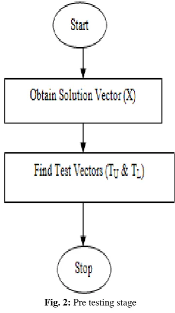
describes the location of a component in the CUT, the test vector is associated to that component and the values are independent of the faults. Thus the fault variable which can be obtained by the element wise division of the difference vector (difference between the nominal and the faulty solutions) and the test vector is also associated to a specific component in the CUT. It is observed that the test vectors are sensitive to the component values and they carry the information regarding the location of the components. In real time, the fault free components may be within the tolerance limits (not exactly the nominal value). The fault detectability is affected if testing is performed with the test vectors simulated with nominal values. To solve this, this paper generates test vectors for lower and upper bound values of components to test the circuit.Fig. 2: Pre testing stage
IV.
SIMULATION
RESULTS
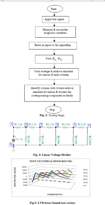
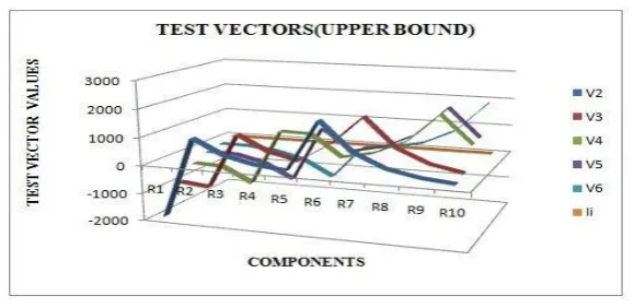
Simulation results on the linear voltage divider (LVD) show the efficiency of the proposed approach. Test vectors are generated for the lower and upper bound values of components and are shown in figure 5 &figure 6. All the components are assumed to have 5% tolerance and the circuit is shown with nominal values in figure 4. Two diagnosis variables measured at the output (node 6 voltage) and input (node 1 current) are used for testing. These variables are selected as they are input and output nodes which are easily accessible for measurement and also the test vectors corresponding to these variables are found to have different value. The fault detectability is affected by the diagnosis variables for which the test vectors are same. The same value test vectors lead to same fault variable, so the faults cannot be distinguished.
Hard faults on passive components of CUT are simulated by assuming 1Ω for short circuit faults and 2×10⁹Ω for hard faults. Single hard faults are injected into the CUT and the diagnosis variables are measured. The fault variables are obtained by measuring the diagnosis variables for the upper and lower bound values of components of CUT (except for faulty component). The average and relative standard deviation relative to the average value are estimated and found to be the lowest value for the faulty component. For example, the short circuit of R1 leads to a fault variable of 8.85E-16 where as for other components of CUT the values are found to
Fig. 3: Testing Stage
Fig. 6: LVD lower bound test vectors
Table 1: Results of Linear Voltage Divider
Fault Type
Relative Standard Deviation of fault variables corresponding to components of CUT Lowest Value of Relative Std. Deviation
R1 R2 R3 R4 R5 R6 R7 R8 R9 R10
R1
Short
8.85E-16 0.95 2.27 2.69 2.8 0.7 1.75 2.6 2.76 2.81 8.85E-16
R2
Short
0.95 1.2 E-15
1.8 2.5 2.8 1.04 1.01 2.3 2.7 2.8 1.2 E-15
R3
Short
2.3 1.8 6.45 E-16
1.8 2.6 2.3 1.02 1.01 2.3 2.7 6.45E-16
R4
Short
2.7 2.6 1.8 1.48E-14 1.8 2.7 2.3 1.03 1.01 1.6 1.48E-14
R8
Short
2.5 2.3 1.01 1.03 2.3 2.6 1.8 5 E-15
0.9 2.2 5E-15
R9
Short
2.8 2.7 2.3 0.95 1.1 2.8 2.6 1.8 3.5 E-15
1.7 3.5E-15
R10
Short
2.8 2.79 2.7 2.3 0.9 2.75 2.8 2.5 1.7 3.9 E-15
3.9E-15
R3
Open
2.3 1.8 5.05E-15
1.8 2.6 2.3 1.02 1.01 1.6 2.5 5.05E-15
R4
Open
2.7 2.6 1.8 8.31 E-15
1.8 2.7 2.3 1.02 1.01 1.6 8.31E-15
R5
Open
2.8 2.76 2.56 1.8 3.9 E-14
2.81 2.7 2.3 1.7 0.9 3.9E-14
R6
Open
0.08 1.02 2.3 2.7 2.8 2.5 E-15
1.8 2.6 2.8 2.81 2.5E-15
R7
Open
1.8 1.01 1.02 2.3 2.7 1.8 6.4 E-15
1.8 2.6 2.76 6.4E-15
V.
CONCLUSIONS
REFERENCES
[1]. Shulin Tian, ChengLin Yang, Fanq Chen, Zhen Liu, “Circle Equation Based Fault Modeling Method for Linear Analog Circuits”, IEEE Transactions on Instrumentation and Measurement, 63 (9):2145-2159, 2014.
[2]. A.D. Spyronasios, M.G. Dimopoulos, A.A. Hatzopoulos,” Wavelet analysis for the detection of parametric and catastrophic faults in mixed-signal circuits”, IEEE Trans. Instrumentation and Measurement, 60, 2025–2038, 2011.
[3]. Hongzhi Hu, Fang Guan, Xin Huang, “Fault Diagnosis of Analog Circuits with Weighted Mahalnobis Distance Based on Entropy Theory”, International Journal of Digital Content Technology and its Applications, Vol.7, No.11, 2013.
[4]. C. L. Yang, S. L. Tian, Z. Liu, J. Huang, and F. Chen, “Fault modeling on complex plane and tolerance handling methods for analog circuits,” IEEE Transactions on Instrumentation and Measurement, vol. 62, No. 10, pp. 2730–2738, 2013.
[5]. Y. Gao, C. L. Yang, S. L. Tian, "Methods of Handling the Aliasing and Tolerance Problem for a New Unified Fault Modeling Technique in Analog-Circuit Fault Diagnosis", Advanced Materials Research, Vol 981, pp. 11-16, 2014.
[6]. Jose A. Soares Augusto and Carlos Beltran Almeida, “ A Tool for Single-Fault Diagnosis in Linear Analog Circuits with Tolerance Using the T-vector Approach”, Hindawi Publishing Corporation, VLSI design, pp 1-8, 2008.
[7]. C.-W.Ho, A.Ruehli and P.Brennan, “The modified nodal approach to network analysis”, IEEE Transactions on Circuits and Systems, Vol.22, no.6, pp.504-509, 1975.