1. An empirical study on regression analysis to predict software effort based on use case points

AN EMPIRICAL STUDY ON REGRESSION ANALYSIS TO

PREDICT SOFTWARE EFFORT BASED ON USE CASE POINTS

1. INTRODUCTION

Software development effort estimates are the basis for project planning, budgeting and bidding. These are demanding practices in the software industry, because poor estimation and planning often has affecting consequences [1]. The common argument on the project cost overruns is very large. Boraso reported that [2] 60% of large projects significantly overrun their estimates and 15% of the software projects are never completed due to the gross misestimating of development effort. Software product delivery on time, within budget, and to an agreed level of quality is a critic concern for software organizations. Accurate estimates are crucial for better planning, monitoring and control [3].

2.1 Linear Regression

Linear regression attempts to paradigmatic relationship between two variables by fitting a linear equation to observed data. One variable is examined to be an explanatory variable, and the other is examined to be a dependent variable. For suppose modeler might want to relate the weights of individuals to their heights using a linear regression model. Before attempting to fit a linear model to observed data, a modeler should first determine whether or not there is a relationship between the variables of interest. This does not necessarily imply that one variable causes the other (for example, higher SAT scores do not cause higher college grades), but that there is some significant association between the two variables. A scatter plot can be a helpful tool in determining the strength of the relationship between two variables. If there appears to be no association between the proposed explanatory and dependent variables then fitting a linear regression model to the data probably will not provide a useful model. A valuable numerical measure of association between two variables is the correlation coefficient, which is a value between -1 and 1 indicating the strength of the association of the observed data for the two variables. A linear regression line has an equation of the form Y = a + b X, where X is the explanatory variable and Y is the dependent variable. The slope of the line is b, and a is the intercept (the value of y when x = 0).

2.2 Multiple Linear Regressions-

Multiple linear regression attempts to model the relationship between two or more explanatory variables and a response variable by fitting a linear equation to observed data. Every value of the independent variable x is associated with a value of the dependent variable y. The population regression line for p explanatory variables x1, x2, ... , xp is defined to

be y = 0 + 1x1 + 2x2 + ... + pxp. This line describes how the mean response y changes with the explanatory variables.

The observed values for y vary about their means y and are assumed to have the same standard deviation. The fitted

values b0, b1, ..., bp estimate the parameters 0, 1, ..., p of the population regression line. Since the observed values

for y vary about their means y, the multiple regression model includes a term for this variation. In words, the model is

expressed as DATA = FIT + RESIDUAL, where the "FIT" term represents the expression 0 + 1x1 + 2x2 + ... pxp. The

"RESIDUAL" term represents the deviations of the observed values y from their means y, which are normally distributed

with mean 0 and variance . The notation for the model deviations is Model for multiple linear regression,

given n observations, is

yi = 0 + 1xi1 + 2xi2 ... pxip + i for i = 1,2, ... n.In the least-squares model, the best-fitting line for the observed data is

1

Research Scholar, Krishna University, Machilipatnam, Asst. Prof in SVEC, TP Gudem

2

HOD, CS Department, Krishna University, Machilipatnam

DOI: http://dx.doi.org/10.21172/1.93.26

e-ISSN:2278-621X

Abstract: - The effort estimation of software development is a process of predicting the most realistic effort (person-hours) required to maintain and development of software. This paper aims to provide best regression technique among linear regression, multi linear regression, exponential regression, and power regression to predict software effort using use case points. The main contribution of this study is a comparative analysis of different regression techniques. To validate the

accuracy of regression techniques we have used R2 _{value, MMRE and TSS. From this study we observed that linear regression,}

calculated by minimizing the sum of the squares of the vertical deviations from each data point to the line (if a point lies on the fitted line exactly, then its vertical deviation is 0). Because the deviations are first squared, then summed, there are no cancellations between positive and negative values. The least-squares estimates b0, b1,... bp are

usually computed by statistical software.

2.3 Exponential Regression using a Linear Model-

Sometimes linear regression can be used with relationships which are not inherently linear, but can be made to be linear after a transformation. In exponential model shown in equation (1)

Y=α (1)

Taking the natural log of both sides of the equation, we have the following equivalent equation (2)

ln y= ln α + βx (2)

This equation has the form of a linear regression model (where I have added an error term ε)

Yʹ=αʹ+βx+ε (3)

2.4 Power Regression using linear model-

Another non-linear regression model is the power regression model, which is based on the following equation

y=α (4)

Taking the natural log of both sides of the equation, we have the following equivalent equation

ln y= ln α + β ln(x) (5)

This equation has the form of a linear regression model (where I have added an error term ε)

Yʹ=αʹ+βxʹ +ε (6)

Observation: A model of the form ln y = β ln x + ε is referred to as a log-log regression model. Since if this equation holds, we have it follows that any such model can be expressed as a power regression model of form y = αxβ by setting α = eδ.

3. RELATED WORK

determining the uncertainty of the estimates. The proposed approach is compared with the basic LSR approach and clustering-based approaches based on industrial datasets.

4. EXPERIMENT RESULTS

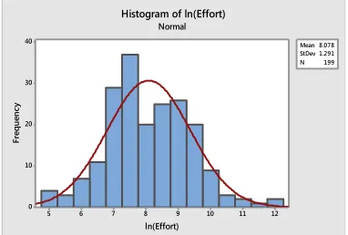
We applied all regression techniques on the data set taken from [12]. The data set contains 214 attributes and Table 1 shows some sample dataset and its attributes. The statistical measures of dataset are given in Table 2. From the Table 2 it can be observed that kurtosis and skewness are very high and data are not properly distributed as shown in Fig 1 and Fig 2. So to apply regression techniques, we have applied logarithmic transformation. From Fig 3 and Fig 4 it can be observed that the data is properly distributed.

Table 1 Sample data set with six attributes

Project number 1 2 3 4 5 6 7 8 9

Complexity value 1 1 0.7 0.7 0.85 1 1 1 0.7

Productivity value 1.3 1.15 1 1.15 1.15 1.15 1 1 1.15

Requirement stability value 1 1 1.2 1 1 1 1 1 1

Size 13.5 18 20.5 28 39 41.5 47 47.5 51

effort 122 296 360 170 507 634 752 751 244

Table 2 Statistical analysis of data set

Sample Size 214

Mean 4.97

Geometric Mean 4.83

Minimum 1.7047

Maximum 8.2965

standard deviation 0.322

Mean Absolute Deviation 1.1771

Standard Deviation 0.9.457

Variance 1.177

Skewness 1.38

Kurtosis 0.1703

3600 3000 2400 1800 1200 600 0 -600 90 80 70 60 50 40 30 20 10 0 Mean 241.9 StDev 407.1 N 198 size Fr eq ue nc y

Histogram of size

Normal

Fig 1 Histogram of independent variable

200000 160000 120000 80000 40000 0 -40000 140 120 100 80 60 40 20 0 Mean7993 StDev 18784 N 198 effort Fr eq ue nc y

Histogram of effort

Normal

Fig 2 Histogram of dependent variable

8 7 6 5 4 3 2 40 30 20 10 0 Mean 4.851 StDev 1.099 N 199 ln(sze) Fr eq u en cy

Histogram of ln(sze)

Normal

Fig 3 Histogram of independent variable ln(size) 12 11 10 9 8 7 6 5 40 30 20 10 0 Mean 8.078 StDev 1.291 N 199 ln(Effort) Fr eq ue nc y

Histogram of ln(Effort) Normal

4.1 Performance evaluation

We evaluate the performance based on Magnitudes of relative error (MRE), mean magnitude of relative error (MMRE) and R2. These are the standard evaluation measures to predict the size and effort estimation. We also used total sum of squares (TSS) which is the metric to evaluate prediction models and median of errors. The following equations have been used for obtaining performance metrics.

MMRE= (1)

= (2)

TSS== 2) (3)

5. SELECTING THE BEST REGRESSION MODELS

The regression equations shown in the Table 3 are derived from MINITAB. We compared linear multi linear, linear power and exponential regression on UCP data.

Table 3 Regression models

Linear regression(LR) 1.15* ln (size)+2.391

Multi Linear

Regression(MLR)

(0.642*ln (size))-0.61*requirement stability+1.64* productivity + 1.22* Complexity-0.322

Power Regression(PR) Ln(size)0.61 *3.07

Exponential

Regression(ER) ( )

Table 4 Statistical measures of regression models

Type of regression model Residual Sum of Squares

Coefficient of

Determination(R2) MEAN

STANDARD

DEVITION MMRE

Linear Regression(LR) 15.0637 91.77 0.045 0.043 0.05

Multi Linear Regression(MLR) 6.63652128 96.374 0.382 0.05 0.38

Power regression(PR) 43.8872 86.486 0.048 0.043 0.047

Exponential Regression(ER) 39.4259 88.4578 0.047 0.044 0.048

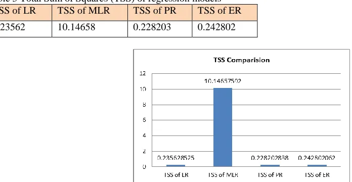
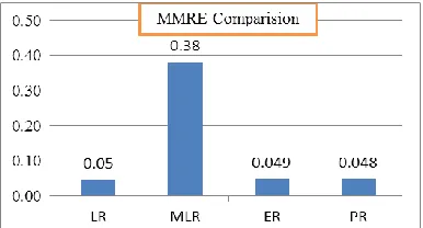
Table 4 shows that the statistical measures of all regression models. Form the table 4 it can be observed that multi linear regression model has highest value of R2 and MMRE. But to select best regression models, we consider one that should have highest R2 and low MMRE values. From our observations linear, power, and exponential regression models have highest R2 and low MMRE values than multi linear regression models. It may be considered that power regression has satisfactory results among all regression models. Fig 5 and Fig 6 show the comparisons of TSS and MMRE values of all regression models respectively.

Table 5 Total Sum of Squares (TSS) of regression models

TSS of LR TSS of MLR TSS of PR TSS of ER

0.23562 10.14658 0.228203 0.242802

Fig 6 MMRE comparisons of regression models

6. CONCLUSION

Software size is one of the important factors that affect the effort estimation. In this paper we studied various regression techniques using use case points to predict the software effort estimation. We applied linear regression, multi linear regression, power regression, and exponential regression on the same data set. We used MMRE, TSS and R2 performance measures to evaluate the accuracy of all techniques. Results have shown that the linear regression, power regression and exponential regression are accurate with little variance than multi linear regression on the test data set.

7. REFERENCES

[1] Crespo, F.J., Sicicila, M.A., Cuadrado, J.J., “On the use of fuzzy regression in parametric software estimation models: integrating imprecision in COCOMO cost drivers”, WSEAS Transactions on Systems, PP. 129-137,Vol.41(2), ISBN: 978-3-540-32780-6, 2004.

[2] Reformat, M., Pedrycz, W., Pizzi, N., “Building a Software Experience Factory Using Granular-Based Models Fuzzy Sets and Systems” Elsevier. 2004.

[3] Xu, Z., Khoshgoftaar, T.M., “Identification of fuzzy models of software cost estimation”, Elsevier Fuzzy Sets and Systems, Vol.145 (1), pp.141- 163, 2004.

[4] Taghavifar, H., and Mardani, “A. Fuzzy logic system based prediction effort: A case study on the effects of tire parameters on contact area and contact pressure”, Applied Soft Computing, pp.390-396, Vol. 14, 2014.

[5] Song, Q., Shepperd, M., and Mair, C. , “Using grey relational analysis to predict software effort with small data sets”, Software Metrics, 11th IEEE International Symposium, pp. 10-35, ISSN: 1530-1435, September 2005.

[6] [6]. Hsu, C. J., and Huang, C. Y., “ Improving effort estimation accuracy by weighted grey relational analysis during

[7] software development” , Software Engineering Conference, 2007. APSEC 2007. 14th Asia-Pacific, pp. 534-541,ISSN: 1530-1362, 2007, December. [8] . Kulkarni, A., Greenspan, J. B., Kriegman, D., Logan, J. J., and Roth, T. D. , “A generic technique for developing a software sizing and effort

estimation model”, In Computer Software and Applications Conference, 1988.

[9] COMPSAC 88 Proceedings, Twelfth International, pp. 155-161, ISBN: 0-8186-0873-0, 1988 October

[10] Grimstad S., Jorgensen, M. and Østvold K.M., “Software Effort Estimation Terminology: The tower of Babel”, Information and Software Technology 48, 2006, pp-302-310, Elsevier.

[11] Boraso M., Montangero C. and Sedehi H., Software Cost Estimation: an experimental study of model performances”, Technical Report: TR-96-22, University of Pisa, Italy.

[12] Wieczorek I. and Ruhe M., “How Valuable is company-specific Data Compared to multicompany Data for Software Cost Estimation?”, Proceedings of the Eighth IEEE Symposium on Software Metrics (METRICS.02).

[13] Nassif, A.B., Ho, D., Capretz, L.F., . Regression model for software effort estimation based on the use case point method. In: 2011 International Conference on Computer and Software Modeling, Singapore, pp. 117–121.2011a

[14] Bou Nassif, Ali, "Software Size and Effort Estimation from Use Case Diagrams Using Regression and Soft Computing Models" (2012).Electronic Thesis and Dissertation Repository. 547.

[15] Briand, L. C., Langley, T., and Wieczorek, I , “A replicated assessment and comparisonof common software cost Modeling techniques”, Proceedings of the 22nd international conference on Software engineering, pp. 377-386,ISBN:1-58113-206-9, 2000.