E-ISSN 2308-9830 (Online) / ISSN 2410-0595 (Print)
Repairing Field Coverage for Static WSNs by Using Mobile Nodes
Ryo Katsuma1 and Yuki Tsuchiya2
1, 2 Graduate school of science, Osaka Prefecture University
1ryo-k@mi.s.osakafu-u.ac.jp
ABSTRACT
In wireless sensor networks (WSNs), sensor nodes periodically sense, record, and transmit environmental information. WSNs require long lifetime and adequate field coverage, which can be problematic under certain conditions. Several studies have addressed these problems using energy harvesting, wireless charging, or mobile sensor nodes. In particular, mobile nodes are effective for adequate field coverage: however, appropriate node movement is critical. In addition, mobile nodes with wireless charging devices can charge the batteries of other nodes. We formulate the problem to extend lifetime and maintain field coverage by determining the positions of mobile nodes that can cover the field effectively and charge the batteries of other nodes simultaneously. We propose a coverage algorithm that can cover a field with a minimal number of nodes and a movement algorithm that determines an efficient mobile node movement schedule to charge static nodes. Simulation results, confirm that the energy charging system used by the proposed method can extend WSN lifetime up to 66%.
Keywords: Wireless Sensor Networks, Mobile Nodes, Network Lifetime, Energy Harvesting, Coverage.
1 INTRODUCTION
Wireless Sensor Networks (WSNs) are networks constructed with many sensor nodes equipped with wireless communication devices. The use of WSNs is expected for a variety of applications, such as environmental monitoring, ecological surveys, and marine guard [1] [2].
A major problem with WSNs is the coverage problem. A sensor node can only sense environmental information within a limited circular sensing range. As a result, node deployment must cover the entire field of interest. Node deployment cost can be reduced by placing nodes at appropriate positions. Several studies have attempted to address this issue by adjusting the position of mobile sensor nodes [13][14]. However, efficient movement scheduling of mobile nodes is required because mobile nodes consume significant amounts of energy when moving.
An other major problem of WSNs is the lifetime extension problem. A WSN is constructed by many sensor nodes that operate with limited battery power. These nodes must be recharged when the power is depleted. Conventionally, wired power supplies are employed to recharge batteries. However, wired power systems cannot be used in general WSNs; thus, operating such WSNs for extended periods is challenging. For example, it is difficult to recharge
WSN node batteries when measuring temperature in a large agricultural field; significant time and costs are required to retrieve, recharge, and redeploy such sensor nodes. Energy harvesting (EH), which converts natural energy (e.g., light and heat) into electricity, has been considered to address this problem. Solar-power and wind-power generation are familiar examples of EH. The strongest point of EH is the ability to charge batteries in several locations, which is otherwise commercially unviable when conventional power charging techniques are employed. In EH, retrieving, recharging, and redeploying sensor nodes are not necessary: thus, it is expected that EH will allow WSNs to operate semi-permanently.
However, energy generation by EH is unstable and sometimes insufficient. Thus, wireless charging technology used for cellular phones and a variety of small devices is our focus. In a wireless charging system, two independent devices are used to send and receive electric power. A node with a sending device consumes energy to charge the battery of a node with a receiving device. It has been reported that electromagnetic induction type wireless charging systems are size and have greater than 80% power efficiency [3].
coverage and charging batteries of static nodes becomes problematic. We have attempted to solve this problem. We propose a method to allow some mobile nodes with sending devices and solar panels to cover the field, and the other mobile nodes charge the exhausted batteries of the static nodes.
The proposed algorithm is comprised of a coverage algorithm and a movement algorithm. When a field is covered by static as well as mobile sensor nodes, the coverage algorithm determines the positions of a minimal number of mobile nodes that can cover the field by determining enclosed regions that are not covered by sensor nodes. The movement algorithm determines the destination points of free mobile nodes. The movement algorithm reduces energy consumption when moving by performing cascade movement [17] in order to avoid moving over long distances.
Our simulation results show that the proposed method extends WSN lifetime up to 66% for a 100 * 100 [m2] field with 20 - 115 nodes. We have confirmed that the coverage algorithm can repair field coverage with a sufficiently small number of nodes. We have also confirmed that employing the proposed method in a diamond deployment pattern is more effective than random deployment.
2 RELATED WORKS
One of the major problems with WSNs is lifetime extension because sensor nodes operate with limited battery power. Recently, many studies have examined using EH technology have to address this problem [4] [8]. In addition, several studies have explored charging node batteries using robots [15] [5].
Brunelli et al. proposed EH technology that uses an efficient and small solar battery module [4]. Their study showed that maximum power point tracking, which can maximize energy generation, allows sensor node batteries to be charged under a variety of solar intensity conditions. The efficiency of power conversion despite the small solar battery was reported to be up to 80%, which is sufficient power generation to charge a sensor node battery. Peng et al. proposed a system that determines charging sequences to be executed by the mobile charger to extend the lifetime of a WSN [5]. However, these studies did not consider field coverage because mobile robots only move for charging.
Another significant problem with WSNs is coverage. For environmental monitoring, it is necessary to cover the target field completely with the minimal number of sensor nodes to enable sensing at any point within the field.
Bai et al. proposed two different deployment patterns, i.e., the diamond pattern and the double-strip pattern. They compared the number of nodes required to achieve field coverage with four-connectivity using these patterns to that of an existing deployment pattern [6]. Other studies have used mobile nodes to cover the field automatically. Wang et al. proposed a field coverage method using mobile nodes that initially move only once to save energy by considering energy balance [7]. However, it is difficult to adapt such methods to changing environments. Eto et al. proposed a method to cover an agricultural field by moving mobile nodes dynamically [8]. Their method avoids battery depletion by predicting the amount of solar energy generation. However, that study targeted WSNs with low sensing frequency where field coverage is achieved by a set of mobile nodes visiting all points in the field at least once during duty cycle. Thus the field is not always covered. Here, the detail of study [7] is explained below.
Existing studies have attempted to solve the lifetime extension problem using EH or wireless charging, or the coverage problem by mobile sensor nodes. Therefore, to address gaps in field coverage and charge static node batteries simultaneously, a new method to determine the efficient loci of mobile sensor nodes is required.
We propose a method that determines the position of each mobile node in order to extend the lifetime of a WSN constructed with static nodes using wireless charging receivers and mobile nodes with wireless charging senders and solar panels.
2.1 Wang’s Algorithm
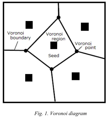
Wang et al. aims to maximize the area covered with a limited number of mobile nodes using Voronoi diagrams. The Voronoi diagram is divided a plurality of points arranged on a plane as shown in Fig. 1 according to which point is the closest. Voronoi diagrams are used in various fields of information processing such as the search of the closest PHS base station. The given point is called seeds. Every seed has its own region called a Voronoi region. In addition, the boundary line of the Voronoi region is called Voronoi boundary, and the intersection of Voronoi boundary is called Voronoi point. As a feature of the Voronoi diagram, the Voronoi boundary is a perpendicular bisector of two seeds, so the Voronoi point is equidistant from the three seeds generating the Voronoi boundary.
Voronoi region and the node in that region is measured. If there is a Voronoi point whose distance is farther than the radius R of the sensing range circle, it means that sensing is not possible in all areas, and this WSN cannot be fully covered. In order to cover the uncovered area, the position of the movable node is determined.
First, a base value b=
(d-R)2 is given to each Voronoi point. Here, d is the distance from the Voronoi point to the nearest node (seed). The mobile node is placed at the position of the Voronoi point where the base value is large. If the distance d between the Voronoi point and the node is largerthan
3
R
, the mobile node is placeed at the position of3
R
from the node on the straight line of the two points. Then, the Voronoi diagram including the mobile node as its generating point is rebuilt and the position where the movable node is placeed again is calculated. This procedure is repeated until the distance between all the Voronoi points and the nearest node is less than or equal to the radius R of the sensing range circle. When all the Voronoi points are within the sensing range of at least one node, the WSN is fully covered.Fig. 1. Voronoi diagram
3 PROBLEM FORMULATION
In this section, we describe the assumptions and the problem formulation.
A. Target WSNs
We target WSNs constructed by a single sink node, static and mobile sensor nodes. A sink node
is denoted by B. Static and mobile sensor nodes have batteries and devices for sensing and radio communication. The capacity of the battery is
denoted by E. The residual battery power of node s
at time t is denoted by s.e(t). The sensing range and communication range are denoted as Rs and Rc, respectively. Both types of sensor nodes sense the environmental data for every duty cycle I (a sink collects the environmental information from all sensor nodes every I minutes). We assume that a mobile sensor node can move to specified destination position, charge its battery by equipped solar panel and send the electric energy to a static sensor node by equipped sending device of wireless charging system. The speed of a mobile node is constant value v. A static sensor node can charge by only its receiving device of wireless charging system. If only the distance between sending and receiving device of wireless charging system is shorter than dc, a static node can charge its battery from a mobile node.
The field which height is Fheight and width is
Fwidth is given. Nstatic static sensor nodes are initially deployed. Then, Nmobile mobile sensor nodes are deployed in order to cover the field completely and charge the battery of static nodes. The position of sensor node s at time t is denotedby
s.pos(t). The destination point of mobile node p at time t is denoted by s.dest(t). A sensor node can know its ownposition and the positions of the other nodes by GPS andwireless communication.
B. Definitions
A sensor node has finite battery and it is not feasible to physically replace the battery upon exhaustion. The battery power is consumed for sensing, moving, wireless communication, and supplying electrinc power. On the other hand, the battery power is charged by solar power genaration and electric power supplied by a mobile node. Consumed power for sensing x[bit] data Sens(x) is expressed by Formula(1).
Sens(x) = xEelec + Esens (1)
Here, Esens and Eelec are constant values that represent the power required by sensing and information processing, respectively.
Consumed powers Trans(x; d) and Recep(x) required to transmit x[bit] for d[m] and receive
x[bit] are expressed by Formulas (2) and (3), respectively [11].
Trans(x,d) = xEelec + xd2eamp (2)
Recep(x) = xEelec (3)
Here, eamp is a constant value that represents the power required by signal amplification.
[m] is expressed by Formula (4) [16].
Move(d) = dEmove (4)
Here, Emove is a constant value that represents the power required to move a node by a distance of 1 [m].
By using the wireless charging system, mobile sensor node p consumes its energy for charging the battery power of static node q. Consumed power
Csend(y) required to send the electric power for y
[sec] is expressed by Formula (5).
Csend (y) = yewc (5)
Here, ewc is a constant value representing the energy consumption by wireless charging system.
The amount of charged energy Crecep(y) by wireless charging system for y [sec] conforms to Formula (6).
Crecep (y) = yzewc (6)
Here, z represents the charging efficiency (0 < z <
1). If z = 1, the energy consumption of a mobile node is equal to the charged energy of a static node. A mobile node can charge its battery by solar power generation. The amount of solar power generated depends on the intensity of solar radiation, which varies according to changing environmental conditions. We denote the intensity of solar radiation at night, during a cloudy day, and during a sunny day as cnight, ccloudy, and csunny, respectively. The amount of solar power generated at the average of solar radiation intensity c([t, t+u]) from time t to t+u is expressed by Formula 7 [8].
Csolar(c[t,t+u]) = esolaruc[t,t+u] (7)
Here, esolar is the coefficient for the amount of energy charged per unit time. c([t, t+u]) conforms Formula (8).
c[t,t+u] = (icnight + jccloudy + kcsunny)
/ (i+j+k) (8)
Here, i, j, and k are the rates of night, cloudy, and sunny time during [t, t + u], respectively.
C. Problem formulation
The inputs for the target problem are target field (Fwidth*Fheight), the positions of a sink node and static nodes, initial battery power of each sensor node, sensing range, constant values Esens, Eelec, eamp, ewc, esolar. The outputs are theposition of each mobile node for each time t and the nodepairs
for battery power supply for each time t. We refer tothis node positions as the node schedule.
Note that the field must always be covered by sensor nodes. Following Formula (9) represents this condition.
pos
Field,
t
T, cover(pos,t)
1 (9)Here, Cover(pos, t) represents the number of nodes covering the point pos at time t.
If node s whose position is s:pos(t) at time t
moves to the s’s destination point s:dest(t), the residual battery amount of s should be larger than the energy consumed for moving. Formula (10) shows this constraint.
t
T, s.energy(t)-Move(|s.dest(t)-s.pos(t)|) + Csolar(c[t,t+|s.dest(t)-s.pos(t)|/v]) >0 (10)Here, T and js:dest(t) � s:pos(t)j represent the WSN termination time and the moving distance, respectively.
If mobile node p charges the battery power of static node q at time t for ut second, the residual battery amount of p should be larger than the energy consumed for charging.
t
T, s.energy(t)- Csend (ut)+ Csola0r(c[t,t+ut]) >0 (11)
Our purpose is to determine the node schedule maximizing WSN operation time T. The objective function is shown in Formula (12).
Maximize(t) (12)
4 PROPOSED METHOD
In this section, we describe the proposed method to solve the target problem explained in Section 3. The proposed method is comprised of two algorithms, i.e., the coverage and movement algorithms.
The coverage algorithm finds uncovered areas and determines the positions of nodes such that the uncovered areas covered filled by a small number of mobile nodes. The movement algorithm periodically determines the movement schedule of the mobile nodes.
4.1 Coverage algorithm
mobile nodes that will cover the uncovered areas. Finally, the mobile nodes are deployed to each position.
To find each uncovered polygon that inscribes an uncovered area, the polygon-finding algorithm finds all uncovered intersections as shown in Fig. 2. An uncovered intersection is an intersection that is not covered by sensor nodes and is made up of two elements, i.e., edges of the target field and sensing range circles of the sensor nodes. Note that an uncovered polygon, whose vertices are uncovered intersections, exists if and only if an uncovered area exists.
Circles are the sensing region of static nodes. Black dots are uncovered intersections.
Uncovered polygons whose vertices are only uncovered intersections are drawn by bold lines.
Fig. 2. Uncovered polygons and intersections
The coverage algorithm minimizes uncovered polygons by placing nodes at appropriate positions in the polygons sequentially until the polygons no longer exist. Here, we denote a set of uncovered polygon vertices found by the polygon-finding algorithm as Q = {q0, q1, q2, ...} , which qi and
qi+1 are adjoined vertices. Two sensor nodes a and
b that construct vertex qi is denoted by qi.s1 and
qi.s2, respectively. Note that qi.s2 and qi+1.s1 represent the same sensor node b. Similarly, qi-1.s2 and qi.s1 represent the same sensor node a. If the distance between qi and qi+2 is within diameter 2Rs of the sensing range circle, the candidate position of a node that covers qi, qi+1, and qi+2 exists. This position is the circumcenter of the triangle whose vertices are qi, qi+1, and qi+2. If no such node position includes these three vertices, the candidate position is the center of the circle that inscribes qi and qi+1. The coverage algorithm places the mobile node at one of these candidate positions such that the area that is newly covered by the mobile node is maximized. Here, if the mobile node placed at the candidate position divides the uncovered polygon into two or more polygons, such a position is eliminated as a candidate. Although one of destination position of optimal
deployment divides the uncovered polygon into two or more polygons, our algorithm puts the node at the position when the destination position no longer divides the uncovered polygon. In order to simplify the problem, our algorithm makes the outer side destination have priority.
For example, uncovered polygon Q is constructed by uncovered intersections q1, q2, q3,
q4, q5, and q6 as shown in Fig. 3 (a). The mobile node is placed at the center of the circle that inscribes q1 and q2, because the area whose size is newly covered by the mobile node is maximized as shown in Fig. 3 (b). Then, the distance between q2 and q4 in Fig. 3 (b) is less than 2Rs, and the mobile node is placed at the circumcenter of the triangle whose vertices are q2, q3, and q4 (Fig. 3 (c)). On the other hand, the mobile node is not placed at a position such that the uncovered polygon becomes divided as shown in Fig. 3 (d).
Fig. 3. A method to cover polygon Q
4.1.1 Coverage algorithm
The output of the coverage algorithm is a set of node positions P. Here, Q is an uncovered polygon.
Q.m is the number of vertices of Q. qi is the i-th element of Q, and dist(qi, qj) is the distance between qi and qj .
1) Find uncovered polygon Q by the polygon-finding algorithm. If no polygon is found, the algorithm terminates.
3) Find i such that dist(qi, qi+2) < 2Rs; otherwise proceed to Step 4. A mobile node is placed at the circumcenter of the triangle whose vertices are qi, qi+1, and qi+2 such that the area that is newly covered is maximized. The coordinate of this mobile node is added to P. Proceed to Step 6. 4) Find i such that dist(qi, qi+1) < 2Rs,
otherwise proceed to Step 5. A mobile node is placed at the center of the circle that inscribes qi and qi+1 such that the area that is newly covered is maximized. The coordinate of this mobile node is added to P. Proceed to Step 6.
5) A mobile node is placed such that the sensing region of the node includes an element of Q and the area that is newly covered is maximized. The coordinate of this mobile node is added to P. Proceed to Step 6.
6) The vertices newly covered by a mobile node are eliminated from Q. The uncovered vertices newly created by a mobile node are added to Q. Return to Step 2.
4.1.2 Polygon-finding Algorithm
The polygon-finding algorithm finds the polygons that are created by the uncovered intersections. The polygon-finding algorithm outputs the uncovered polygon Q. Here, P is a set of uncovered intersections.
1)i = 0. If P = ∅, the algorithm terminates as no polygon is found.
2)If qi.s2 is an edge of the field, proceed to Step 4, else go to Step 3.
3)Investigate the element of P to way that is not covered by qi.s1 in the sensing range circle. The point that is found first is qi+1. Proceed to Step 5.
4)Investigate the element of P to way that is not covered by qi.s1 on the edge of the field. The point that is detected first is qi+1.
5)If qi+1.s1 is not qi.s2, exchange qi+1.s1 with
qi+1.s2.
6)If qi+1 is p0, proceed to Step 7, else i = i + 1 and return to Step 2.
7)All followed points except qi+1 are added to
Q. The algorithm terminates with P = P - Q.
4.2 Movement algorithm
The movement algorithm allows field coverage to be maintained for long periods. We set two modes for each mobile node, i.e., a coverage mode and a free mode. A coverage mode mobile node moves to the candidate position calculated by the coverage algorithm. Note the number of coverage mode nodes is fixed. The other nodes operate in free mode. If the residual battery power of a coverage mode node becomes low, the free mode node moves to the position of the coverage mode node and becomes a coverage mode node. Note that free mode nodes do not perform sensing.
In the movement algorithm, nodes communicate residual battery power and power-generation efficiency information to each other, and the sink node forecasts node s whose residual battery power will be depleted rapidly. If s is a free mode node, s
charges its battery by solar power at its current position. If s is a static node or a coverage mode node, it seeks another mobile node n1 with sufficient battery power. If mobile node n1 is a free mode node, then it moves to the position of node s
and performs wireless charging or changes n1’s
mode to coverage and s’s mode to free: otherwise, s
seeks the nearest free mode node n2. Ecn1 and
Ecn2 are the estimated residual battery power of
nn1 and nn2 when n2 move to the position of n1 and nn1 moves to the position of s (this type of movement is referred to as cascade movement [17]. Ed n1 and Ed n2 are the estimated residual battery power of nn1 and nn2 when n2 moves directly to the position of s. The movement algorithm compares the minimum values of the estimated residual battery power Ecn1 and Ecn2 to
Ed1 and Ed2 by these two movement types and selects the movement type with greater estimated residual battery power.
The movement algorithm runs when a node whose residual battery power is less than L/l exists. Here, the average residual battery power among all nodes is denoted L.
4.2.1. Movement algorithm
1) If node s whose residual battery power is a less than L/l is free mode node, then s’s
battery is charged by solar energy generation and the algorithm terminates, else seek the nearest mobile node n1 whose battery power is greater than L.
battery power and is the nearest node from s.
3) Estimate the residual battery power Ed n1 and Edn2 bymoving n2 to the position of s
directly, and estimate Ec1 and Ec2 by moving n2 to n1’s position and n1 to the position of s (cascade movement).
4) Select the movement of the greater minimum value of Ec1 and Ec2, or Ed1 and Ed2. Mobile nodes are then moved.
5) If node s is a static node, the moved mobile node performs wireless charging, else s and the moved mobile node exchange modes.
5 PERFORMANCE EVALUATION
Here, we describe simulation results of an evaluation of the proposed method.
We performed computer simulations to measure the field coverage time that can be maintained by varying the number of sensor nodes for two patterns of static sensor node deployment. In the first scenario, static sensor nodes are scattered by a helicopter, i.e., they are deployed randomly. The mobile sensor nodes primarily move to fill gaps in field coverage. In the second scenario, static sensor nodes whose batteries have less than one-half charge are deployed in a diamond deployment pattern. In this scenario, the deployment is calculated and efficient, and the WSN is used for a long period. Mobile sensor nodes primarily move to charge static sensor node batteries and repair coverage holes.
5.1 Coverage algorithm evaluation
In this simulation, n static nodes were deployed initially, and the number of mobile sensor nodes required for complete field coverage was measured. We compared the proposed method with Wang's method [7]. In this simulation, the target field is set to 100 * 100 [m2], and the sensing range radius is set to 20 [m], respectively.
5.1.1 Comparison of collapse degree of coverage due to error of node position
When actually placing a node, deviation may occur due to error of position estimation such as GPS etc. In theory, even in the state that the entire coverage is possible, there are cases where it is not possible to cover the whole in practice. Therefore, the shift width of the node position and the number of occurrences of the uncovered area at that time are measured. In this experiment, after using the coverage algorithm and the covering method of Wang et al., respectively, a mobile node is placed at
the position of the node covering all the target area, and then all nodes are randomly distanced within a range of n [m]. The number of polygons generated at uncoated intersection points that can be made by shifting in the direction is measured. The number of fixed nodes is 10, and the initial positions of fixed nodes for both methods are the same. The range of shifting the nodes is within 0.5, 1, 2, and 3 [m], respectively.
Fig. 4. The number of uncovered polygon newly generated by node shift
Fig. 4 shows an average value obtained by performing this experiment ten times for each shiftable range of nodes. We confirmed that the number of polygons is smaller in Wang et al. In the proposed method, the number of polygons increases as the range of shift increases, but the number of polygons by the covering method of Wang et al. does not change so much. As a result, it can be seen that the covering method of Wang et al. has tolerance to node shift. Since the proposed method places the mobile node so that the uncovered intersection and the coverage area border are in contact with each other, there is a high possibility that coverage cannot be achieved even if the node slightly shifts, and the number of polygons tends to increase.
5.1.2 Comparison of the number of nodes required for entire coverage
Fig. 5. The number of nodes required for entire field coverage
Fig. 5 shows the average value of the number of movable nodes added to cover the target area by performing this experiment ten times for each fixed node number. In all cases, we found that the proposed method had about 20% less number of mobile nodes to add. The difference becomes larger as the number of fixed nodes becomes smaller, and we confirmed that the proposed method is effective. The reason for this is considered to be that in the method of Wang et al., the area covered by one mobile node is placed to be large. Since the uncovered region is finely divided as shown in Fig. 3 (d), the number of holes in the coverage may be increased, and the nodes are placed individually for these holes. From the above results, when comparing the proposed method and the covering method of Wang et al., the proposed method has more holes in the coating than the covering method of Wang et al. due to node shift, and can reduce the number of nodes required for the total coverage about 20%. However, in the proposed method, the area of the hole of the coverage caused by the misalignment of the node is very small, and the total coated area hardly changes.
5.1 Evaluation for extending lifetime
In this simulation, we measured the lifetime of the WSN by changing the number of static or mobile sensor nodes. WSN operation was terminated when battery power of at least one node was depleted.
Table 1: Parameters
Parameter Value
Size of target field 100*100 [m2] Sensing radius Rs 20 [m]
Duty cycle I 15 [min]
Data size 256 [bit]
Battery capacity E 8640 [J] Power consumption
coefficient for data processing Eelec
50 [nJ/bit]
Power consumption coefficient for signal amplification eamp
100 [pJ/bit/m2]
Power consumption coefficient for sensing
Esens
0.018 [J/bit]
Power consumption for moving
1680 [mW]
Efficiency of wireless charging z
0.8
5.2.1 Changing the number of mobile nodes
To evaluate the effects of the proposed features, we compared the proposed method with a method whose battery charging mechanism has not been validated (hereafter, simple method). The common parameter settings in our simulations are shown in Table 1. The network topology is a mesh rooted at the sink node. Each sensor node sends data to the upper node that has maximum residual battery power.
Fig. 6. Network lifetime for 15 static nodes
5.2.2 Diamond deployment pattern
Fig. 7. Diamond deployment pattern
WSNs are sometimes required to operate according to planned node deployment. In this simulation, each static sensor node was deployed as the center point of a hexagon inscribed in a circle whose radius is Rs, as shown in Fig. 7. The diamond deployment pattern shown in Fig. 7 is the most efficient deployment [12]. The diamond pattern requires 14 static nodes to cover a 100 *
100 [m2] field.
We added mobile sensor nodes to WSNs constructed with only static sensor nodes that have already consumed one-half and one-quarter if their battery power on average. The durations from initial deployment of the static nodes until one-half and one-quarter battery power was consumed was 189.4 [h] and 298.7 [h], respectively. Here, we describe these two cases (i.e., half and one-quarter battery consumption). For each case, we measured the lifetime extension achieved by adding mobile nodes.
Figures 8 and 9 show the half and one-quarter cases, respectively. As can be seen in both figures, the proposed method extends WSN lifetime linearly relative to the number of mobile nodes.
However, the degree of lifetime extension is gradual around 550–600 [h]. With 30 mobile nodes, Figs. 6 and 8 show 793.2 [h] and 591.5 [h] lifetime extensions. In the one-half case, the WSN lifetime is 591:5 + 189:4 = 780:9. Although no mobile node was used for 189.4 [h], the lifetime of the one-half case was similar to the randomly deployed case. In Fig. 9, the lifetime of 30 mobile nodes is less than 25 mobile nodes. The reason is the deviation of initial energy amount. Our simulations conducted 10 times were not able to eliminate the affect of unfortunate initial parameters. Thus, we confirmed that the proposed method with a diamond deployment pattern can extend WSN lifetime.
Fig. 8. Network lifetime for 1/2 case in diamond deployment pattern
Fig. 9. Network lifetime for 1/4 case in diamond deployment pattern
5.2.3 Without battery charging
with wireless charging function has longer operation time. As a result, using the wireless charging technology is effective when the number of mobile nodes is small. We also confirmed that it can preferentially charge nodes with high power consumption (important on the network).
Fig. 10. Network lifetime without battery charging
6 CONCLUSION
We have proposed a method to extend WSN lifetime using two energy charging systems. The proposed algorithm includes a coverage algorithm and movement algorithm. The coverage algorithm determines the positions of mobile nodes that cover areas not covered by static nodes. The movement algorithm determines the destination of nodes whose batteries need to be charged by mobile nodes. Our simulation results, confirm that the proposed method with a diamond deployment pattern can extend WSN lifetime. As a result of comparison with the existing method, we confirmed that the existing method is more tolerant to the position error of the node, but the proposed method can reduce the number of nodes required to cover the uncovered region by about 20%.
6 REFERENCES
[1] Th.Aramapatzis, J.Lygeros, and S. Manesis, : “A Survey of Applications of Wireless Sensors and Wireless Sensor Networks,” Proceedings of International Symposium on, Mediterrean Conference on Control and Automation (ISIC/MED 2005), pp. 719- 724 (June 2005). [2] A. Mainwaring, D. Culler, J.Polastre, R.
Szewczyk, and J.Anderson;“Wireless sensor networks for habitat monitoring ,” Proceedings of the 1st ACM International Workshop pn Wireless Sensor Networks and Applications, pp.88-97 (2002).
[3] HIDEKI AYANO, HIROSHI NAGASE, HIROMI INABA, : “A Highly Efficient Contactless Electrical Energy Transmission
System,” Electrical Engineering in Japan, Vol 148, No.1, 2004.
[4] Davide Brunelli, Luca Benini, Clemens Moster, and Lothar Thiele: “An Efficient Solar Energy Harvester for Wireless Sensor Nodes,” Proceedings of the conference on Design, automation and test in Europe, pp. 104-109, (2008)
[5] Yang Peng, Zi Li, Wensheng Zhang, and Daiji Qiao, : “Prolonging Sensor Network Lifetime Through Wireless Charging,” IEEE Real-Time Systems Symposium (RTSS), San Diego, CA, November 30 - December 3, 2010.
[6] Xiaole Bai, Ziqiu Yun, Dong Xuan, Ten H. Lai, and Weijia Jia:“Optimal Patterns for Four-Connectivity and Full Coverage in Wireless Sensor Networks,” Mobile Computing, IEEE Transactions on (Volume:9, Issue: 3 ) pp. 435-448, March 2010
[7] You-Chuin Wang, Wen-Chium Peng, and Yu-Chee Tseng, : “Energy-Balanced Dispatch of Mobile Sensor in a Hybrid Wireless Sensor Network,” IEEE Transactions on Parallel and Distributed Systems, vol.21, no. 12, pp. 1836-1850, Dec. 2010
[8] Masaru Eto, Ryo Katsuma, Morihiko Tamai, and Keiichi Yasumoto:“Efficient Coverage of Agricultural Field with Mobile Sensors by Predicting Solar Power Generation,” Proc. of IEEE Int’l. Conf. on The 29th IEEE International Conference on Advanced Information Networking and Applications (AINA), pp. 62–69, 2015.
[9] M. Cardei, J. Wu, M. Liu, and M. Pervaiz: “Maximum network lifetime in wireless sensor networks with adjustable sensing ranges,” Proc. of IEEE Int’l. Conf. on Wireless and Mobile Computing, Networking and Communications (WiMob), 2005.
[10]Jiong Wang, Medidi, S., Medidi, M.: “Energy-Efficient k-Coverage for Wireless Sensor Networks with Variable Sensing Radii ,” Proc. of IEEE Int’l. Conf. on Global
Telecommunications Conference
(GLOBECOM), pp. 1–6, 2009.
[11]Heinzelman, W.R., Chandrakasan, A., Balakrishnan, H. “Energyefficient communication protocol for wireless microsensor networks,” Proc. of the 33rd Hawaii Int’l. Conf. on System Sciences (HICSS 2000), pp.1–10, 2000.
[13]Luo, R.C., and Chen, O.: “Mobile Sensor Node Deployment and Asynchronous Power Management for Wireless Sensor Networks,” IEEE Trans. on Industrial Electronics, No. 59, Vol. 5, pp. 2377–2385, 2011.
[14]Wang, Y. C. and Tseng, Y. C.: “Distributed Deployment Schemes for Mobile Wireless Sensor Networks to Ensure Multi-level Coverage,” IEEE Trans. on Parallel and Distributed Systems, No. 19, Vol. 9, pp. 1280– 1294, 2007.
[15]Ouadou, Mourad, Zytoune, Ouadoudi, and Aboutajdine, Driss:“Wireless charging using mobile robot for lifetime prolongation in sensor networks,” Proc. of IEEE Complex Systems (WCCS), pp. 225–230, 2014.
[16]Rahimi, M., Shah, H., Sukhatme, G.S., Heideman, J., Estrin, D. “Studying the Feasibility of Energy Harvesting in a Mobile Sensor Network,” Proc. of the IEEE Int’l. Conf. on Robotics and Automation (ICRA), pp.19–24, 2003.