Level Control of Conical Tank using Model Free Adaptive Control

IJIRT 101589

230

Level Control of Conical Tank using Model Free Adaptive

Control

Sam Varghese, Rajalakshmy P.

Department of Electronics and Instrumentation

Karunya University, Coimbatore, India

Abstract—A model free adaptive control with estimated pseudo

partial derivative (PPD) is introduced by multi-input fuzzy rules emulated network (MiFREN) for a Conical tank system. The Parameters adaptation scheme ensures a satisfactory settling time. Human knowledge about the controlled plant is rearranged to define the IF-THEN rules directly. Those fixed parameters are designed according to guarantee the convergence related on the controller performance. All adjustable parameters inside MiFREN are tuned by the proposed on-line learning algorithm. The simulation result demonstrate the performance of the proposed controller for the system.

Index Terms—model free, fuzzy, on-line learning, pseudo partial derivative.

I. INTRODUCTION

Model free adaptive control (MFAC) has been continuously developed for several systems with unknown or ill-defined model especially for a class of discrete-time domain. Without any mathematic model of the plant, a linearization concept based on pseudo-partial derivative (PPD) is composed as the equivalent system. Due to the comparison with other adaptive controllers, only real time measured data of the controlled plant is necessary to establish MFAC. Unlike model reference adaptive control based on neural networks, the off-line tuning phase can be excluded because the time-varying PPD can be tuned by real time measurement data only.

In general, the control law has been determined by PPD under some necessary constrains and the resetting technique. It’s clear that the control system performance depends on the accuracy of PPD estimation. The compensation system based on an artificial neural network has been discussed in by the additional of another control effort. By using the on-off controller, the system dynamics can be considered as the unknown system when the switching sequence can be adapted by a feedback controller.

According to the controlled plant, in practice, PPD seems like the system sensitivity which can be understood by human knowledge related on input-output behavior. In this work, this knowledge can be reformulated into IF-THEN rules for an adaptive network called “multi-input fuzzy rule emulated network” (MiFREN). The on-line adaptation is developed to tune all adjustable parameters inside MiFREN. Thus, the time variation of PPD can be directly estimated by MiFREN according to our proposed cost function. Moreover, the resetting algorithm, which is needed for tuning PPD, can

be relaxed in this work because of MiFREN’s property which is directly related on the change of input respectively to the plant’s output. All fixed parameters are designed to guarantee the convergence which can affect the performance of controller.

II. CONICAL TANK

2.1 Modeling and System description

In this level process the tank is conical shape in which the level of liquid is desired to maintain at a constant value .This is achieved by controlling the input flow into the tank. The control variable is the level in a tank and the manipulated variable is the inflow to the tank. Conical tank is non-linear in nature because of its varying cross-sectional area. For industries using non-linear processes the controller design is a challenging task, because majority of the control theory deals with linear process. Many industries use proportional controller (PI) and proportional integral derivative controller because of its simple structure and easy tuning. They are perfect control for linear process. Tuning of the controller is setting the proportional, integral and derivative constant to get the best control of the process. The conical tank is highly non-linear. But stability of the system may be affected.

2.2 Plant Model for simulation purpose

Q - Flow rate of the inlet stream Qo - Flow rate of the outlet stream R - Maximum radius of the conical tank

r - Radius of the conical tank at steady state

H - Maximum height of the conical tank

h - Height of the conical tank at steady state

The mathematical modelling of the system should be obtained using the process parameters.

According to mass balance equation, Accumulation = Input- Output,

So that the tank model becomes,

Where and are parameters defined by,

Here, Q is the inlet flow rate, the manipulated variable. This process model has two types of nonlinear functions: Qh-2, a product of two functions, and h-3/2.These two functions have to be linearized. Linearization is the process by which a nonlinear system is approximated to a linear process model. The most popular technique for obtaining the linear approximation is based on Taylor series expansions of the nonlinear aspects of the process model.

The linearization of f (h, Q) =Qh-2 proceeds as follows,

Ignore the higher order terms,

Under steady state condition, . Now introduce the variables y= (h-hs) and u = (Q-Qs). The approximate linear model is obtained as,

III. CONTROL SYSTEM DESIGN

3.1 Fuzzy Control System

A fuzzy control system is a control system based on fuzzy logic—a mathematical system that analyzes analog input values in terms of logical variables that take on continuous values between 0 and 1, in contrast to classical or digital logic, which operates on discrete values of either 1 or 0 (true or false, respectively).

Fuzzy logic is widely used in machine control. The term "fuzzy" refers to the fact that the logic involved can deal with concepts that cannot be expressed as "true" or "false" but rather as "partially true". Although alternative approaches such as genetic algorithms and neural networks can perform just as well as fuzzy logic in many cases, fuzzy logic has the advantage that the solution to the problem can be cast in terms that human operators can understand, so that their experience can be used in the design of the controller. This makes it easier to mechanize tasks that are already successfully performed by humans.

Fuzzy logic was first proposed by “Lotfi A. Zadeh” of the University of California at Berkeley in a 1965 paper. He elaborated on his ideas in a 1973 paper that introduced the concept of "linguistic variables", which equates to a variable defined as a fuzzy set. Other research followed, with the first industrial application, a cement kiln built in Denmark, coming on line in 1975.

The input variables in a fuzzy control system are in general mapped by sets of membership functions similar to this, known as "fuzzy sets". The process of converting a crisp input value to a fuzzy value is called "fuzzification". A control system may also have various types of switch, or "ON-OFF", inputs along with its analog inputs, and such switch inputs of course will always have a truth value equal to either 1 or 0, but the scheme can deal with them as simplified fuzzy functions that happen to be either one value or another.

3.2 Problem Foundation

In this work, the nonlinear system for a class of discrete time domain can be described by,

where y(k) ϵ R and u(k) ϵ R denote as the time index k system output and input, respectively with the unknown order ny and nu. The non-linear function f(.) is definitely unknown. According to the conventional MFAC algorithms, those following assumptions are stated.

IJIRT 101589

232

Assumption 2: The non-linear system described in the

equation above is generalized Lipschitz. That means the positive constant lmust be defined when,

│Δy(k+1)│ ≤ l│Δu(k)│, when Δy(k+1) = y(k+1) – y(k) and Δu(k) = u(k) – u(k-1).

According to those upper assumptions, the following lemma can be obtained.

Lemma 1: The non-linear system satisfied assumption 1 and 2

with │Δu(k)│≠ 0 for time index k, can be transformed into the equivalent compact form dynamic linearization (CFDL) as, Δy(k+1) = ɸ(k) Δu(k), (2) where ɸ(k) denotes the pseudo partial derivative (PPD). The parameter PPD can be estimated by several learning algorithm such as the modified projection. On the other hand, in this work, PPD is determined by the adaptation network MiFREN which can be operated under the human knowledge according to the controlled plant.

3.3 Control Law

Let the cost function be defined as,

when λ is a designed weighting constant. By using (1), the cost function can be rewritten as,

Differentiating (4) with respect to u(k),

The idea control law can be obtained as,

In practice, the output y(k) can be measured but ɸ(k) cannot be directly determined because of the unknown non-linear system f(.). To realize this control law, ɸ(k) will be estimated

by MiFREN as , thus the control effort can be generated by,

when ρ is a step-size constant. Both ρ and λ are designed parameter which can be given by the following lemma to guarantee the convergence of u(k). Before the proof of control effort boundary, the following assumption is necessary.

Assumption 3: The direction of or sign { } is

unknown but it doesn’t change as sign { }=sign

{ }.

Lemma 2: According to assumption 2 and the MiFREN’s

property, the maximum of must be existed as

and both parameters ρ and λ are designed by following this relation,

thus, the control effort from (8) is bounded.

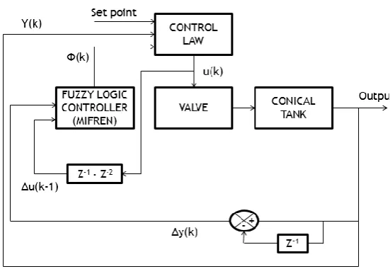
Model Free Adaptive Control

Fig 3.1: Model Free Adaptive Control

The diagram above shows the basic working of the system created. The on-line data from the plant are fed to the Control Law. The Fuzzy Logic Control (MiFREN) provides its output to the Control Law as well using the data from the plant. Finally, the control u(k) is generated from the Control Law and provided as input to the Valve. The Valve in turn controls the Conical tank so as to reach the desired set point.

3.4 MiFREN for pseudo partial derivative

3.4.1 PPD based on MiFREN

MiFREN is an adaptive network which can be operated by human knowledge in the format of IF-THEN rules. The design of IF-THEN rules is also a key of the performance. The knowledge based on the controlled plant is roughly necessary. The relation can be rearranged as,

With this implementation, unlike the conventional algorithms

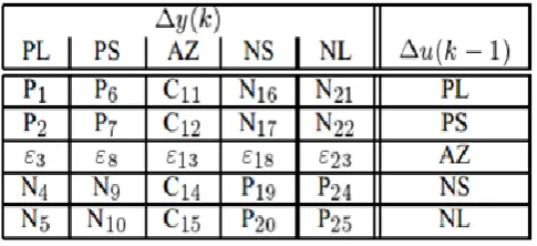
to determine , the sign of is directly determined by those IF-THEN rules. To simplify, those IF-THEN rules can be defined by Table 1.

Table 1: IF-THEN Rules

The linguistic variables PL, PS, AZ, NS and NL denote as Positive Large, Positive Small, Almost Zero, Negative Small and Negative Large, respectively. In this case, the number of IF-THEN rules is 25 and the relation the THEN-part can be given by other linguistic variable. The variables P, C and N stand for Positive, Close to zero and Negative, respectively.

Unlike the conventional technique, when nearly reaches to zero or stays in the range to AZ-membership function, the designed parameter ɛ3 = ɛ8 = ɛ13 = ɛ14 = ɛ23 = ɛ.

The Fuzzy rules were created according to the PPD relation mentioned above. Two input variables were defined: “del-y” and “delprevcntrleffrt”. One output variable was defined: “valve”. All the variables were given 5 membership functions each: NL, NS, ZERO, PS and PL. The Fuzzy rules are:

Fig 3.2: IF-THEN Rules

IJIRT 101589

234

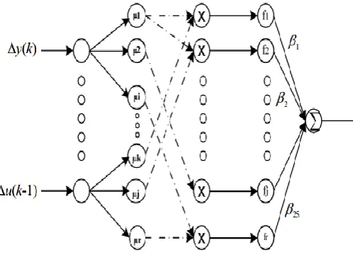
Fig 3.3: The structure of MiFREN

Layer 1: Each input in this layer is sent to the corresponding nodes in the next layer directly. Thus there is no computation in this layer.

Layer 2: This is called the input membership function (MF) layer. Each node in this layer contains a membership function corresponding to one linguistic level (e.g. negative, nearly zero, etc.). The output at the i-th node for the input is denoted by

Layer 3: This layer corresponds to the fuzzy inference. The number of nodes in this layer is rn nodes. The output signal at each node in the layer is calculated as,

Layer 4: This layer may be considered as a defuzzification step. It is called the Linear Consequence (LC) layer. There are also rn nodes in this layer.

Layer 5: The structure of this layer is similar to the output layer of an artificial neural network with unity weight. The output of the MIFREN,

“βi” is a Linear Consequence (LC) parameter for THEN-part linguistic variables. The Function F(.) is the ith rule relation determined by membership functions related on the ith rule. For example, according to Table 1, we have F1(k) = µPL(Δy(k))µPL(Δu(k-1)) at rule # 1, F16(k) = µNS(Δy(k))µPL(Δu(k-1)) at rule # 16 and F25(k) = µNL(Δy(k))µNL(Δu(k-1)) at rule # 25.

3.4.2 Parameters Adaptation

The on-line learning algorithm will be applied in this work for LC parameters. Thus, the estimated PPD can be rewritten by,

when βi(k) denotes the LC parameter for the ith rule at time

index k. To tune this parameter, the cost function can be given as the following,

where γ is defined as a small positive constant. Determining the derivative with respect to βi(k), we obtain,

According to Gradient Search, the tuning law can be defined by,

where, ηB is the learning rate which can be designed as a small positive constant. By using the above two equations, the tuning law can be formulated as,

The designed paramters γ and ηB can effect to the convergence of β.

IV. SIMULATION RESULTS AND DISCUSSIONS

4.1 MATLAB

MATLAB (matrix laboratory) is a multi-paradigm numerical computing environment and fourth-generation programming language. Developed by MathWorks, MATLAB allows matrix manipulations, plotting of functions and data, implementation of algorithms, creation of user interfaces, and interfacing with programs written in other languages, including C, C++, Java, Fortran and Python.

Although MATLAB is intended primarily for numerical computing, an optional toolbox uses the MuPAD symbolic engine, allowing access to symbolic computing capabilities. An additional package, Simulink, adds graphical multi-domain simulation and Model-Based Design for dynamic and embedded systems.

Libraries written in Perl, Java, ActiveX or .NET can be directly called from MATLAB, and many MATLAB libraries (for example XML or SQL support) are implemented as wrappers around Java or ActiveX libraries. Calling MATLAB from Java is more complicated, but can be done with a MATLAB toolbox which is sold separately by MathWorks, or using an undocumented mechanism called JMI (Java-to-MATLAB Interface), (which should not be confused with the unrelated Java Metadata Interface that is also called JMI).

As alternatives to the MuPAD based Symbolic Math Toolbox available from MathWorks, MATLAB can be connected to Maple or Mathematica. Libraries also exist to import and export MathML.

4.2 Fuzzy Control Logic

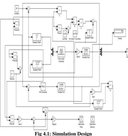
Simulation using Fuzzy is done using MATLAB as shown in the figure below:

Fig 4.1: Simulation Design

The diagram above shows the Simulation design. It includes the Control Law calculation and a part of the Parameters adaptation. A PID controller is used with the system just for comparison with the ‘System response using Fuzzy’. A part of the calculation for parameters adaptation is given to Data Store Write block for transferring the values from here to the subsystem for further calculation.

4.2.1 Modifications within Fuzzy block

The default Fuzzy wizard of the Fuzzy logic block in Simulink was modified to a MiFREN network.

Fig 4.2: Modified Fuzzy Block

So as to implement the MiFREN network within the Fuzzy system, the masked subsystem of the Fuzzy block in Simulink had to be modified. The subsystem shown above was present within the “Fiz Wizard”. Since 25 rules were given to the block, there were 25 lines present. Each output from the rule block was taken, defuzzified separately, demuxed and then used in calculation to obtain the correct value of the weight, βi. Finally, all the β values were summed and given to the output.

4.2.2 Subsystem created for Parameters Adaptation

The system below is a part of the Tuning law for the convergence of β.

Fig 4.3: Subsystem for Parameters Adaptation

IJIRT 101589

236

Repeated iterations as in the equation resulted in a singularity error. Hence, a limited number of iterations were performed so as to implement the equation. A Data Store Memory block from Simulink was used to transfer values from the model to the Fuzzy subsystem.

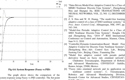
4.2.3 System Response (Fuzzy vs PID)

Fig 4.4: System Response (Fuzzy vs PID)

The graph above shows the comparison of the System response using Fuzzy vs PID controller. The Set-point here given is 50 cm. As it can be seen above, the Fuzzy response has no oscillations compared that of PID controller.

4.3 PERFORMACE ANALYSIS

The response from the system using Fuzzy Logic System showed better results. In comparison to the response from the system using PID controller, the output using MiFREN network had no oscillations with settling time almost equal to that of the system with PID.

V. CONCLUSION AND FUTURE WORK

The MATLAB program was designed and simulated for the Conical Tank system using Fuzzy Logic Controller. The first phase was to develop the Control Law for the generation of PPD (Partial Pseudo Derivative). After implementing the control law within the design, the default Fuzzy logic within the Fuzzy block from Simulink was modified to make it a MiFREN network. The second phase was to create the Parameters adaptation design. In order to proceed with the adaptation, a subsystem was created and added to the MiFREN network. The response from the system

was satisfactory. Also, the system response using PID was shown for comparison. The response using Fuzzy showed no oscillations.

As for the Future work for this project, Neural-Fuzzy network can be used to perfect the response from the system. Also, the number of Fuzzy rules can be increased to obtain better results.

References

[1] “Data-Driven Model-Free Adaptive Control for a Class of MIMO Nonlinear Discrete-Time Systems”, Zhongsheng Hou and Shangtai Jin, IEEE TRANSACTIONS ON NEURAL NETWORKS, VOL. 22, NO. 12, DECEMBER 2011

[2] Z. S. Hou and W. H. Huang, “The model-free learning adaptive control of a class of SISO nonlinear systems,” in Proc. Amer. Control Conf., Albuquerque, NM, 1997, pp. 343–344.

[3] “Model-free Periodic Adaptive Control for a Class of SISO Nonlinear Discrete-Time Systems”, Ronghu Chi and Zhongsheng Hou, “2010 8th _{IEEE International} Conference on Control and Automation, Xlamen, China, June 9-11, 2010

[4] “Controller-Dynamic-Linearization-Based Model Free Adaptive Control for Discrete-Time Nonlinear Systems“, Zhongsheng Hou ; Adv. Control Syst. Lab., Beijing Jiaotong Univ., Beijing, China ; Yuanming Zhu

[5] “Model free adaptive control with pseudo partial derivative based on fuzzy rule emulated network”,

Chidentree Treesatayapun, Department of Robotic and Advanced Manufactory, CINVESTAV -Saltillo, Ramos Arizpe, 25900, Mexico