Improved Speech Recognition Processes Using
Hybrid Genetic Vector Quantization
1
Randeep,
2Priyanka Jaglan
1,2Dept. of ECE, Guru Jambheshwar University of Science and Technology, Hisar, Haryana, India
Abstract
Speech recognition basically means talking to a computer, having it recognize what speakers are saying. Speech is common and
efficient form of communication method for people to interact with
each other. The person would also like to interact with computer via speech. It can be accomplished by speech recognition system
in which computer identifies the word spoken by a speaker into a
microphone. Speech recognition is becoming more complex and a challenging task. The research is focusing on large vocabulary, continuous speech capabilities and speaker independence. This paper reviews methods and technologies available for ASR process
Keywords
Speech Recognition, ASR, Feature Extraction, Speech Models
I. Introdution
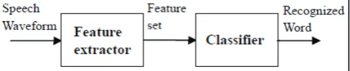
Speech recognition systems have a expansive scope of requests from isolated-word recognition as in term dialing and voice-control of mechanisms to constant usual speech recognition as in auto-dictation or broadcast-news transcription [1]. Most useful speech recognition systems encompass of two modules: the front conclude feature module and back conclude association module. Fig. 1 displays a general scheme of a speech recognition system.
Fig. 1: General Scheme of a Speech Recognition System
The task of ASR is to take an acoustic waveform as an input and produce output as a string of words. Basically, the problem of speech recognition can be stated as follows. When given with acoustic observation X = X1, X2…Xn, the goal is to find out the
corresponding word sequence W = W1, W2…Wm that has the maximum posterior probability P(W|X) expressed using Bayes
theorem as shown in equation (1). The following fig. 2 shows the
overview of ASR system
Where P(W) is the probability of word W uttered and P(X|W) is the probability of aural observation of X after the word W is uttered.
In order to understand speech, the arrangement normally consists of two phases. They are shouted pre-processing and post processing. Pre-processing involves feature extraction and the post-processing period embodies of constructing a speech recognition engine. Speech recognition engine normally consists of vision concerning constructing an aural ideal, lexicon and grammar. After all these
features are given accurately, the recognition engine identifies
the most probable match for the given input, and it returns the understood word.
Fig. 2: Overview of ASR System
A vital task of growing each ASR arrangement is to select the suitable feature extraction method and the recognition approach. The suitable feature extraction and recognition method can produce good accuracy for the given application. Hence, these two main constituents are studied and contrasted established on
its merits and demerits to find out the best method for speech
recognition system. The assorted kinds of feature extraction and
speech recognition ways are clarified in the pursuing section.
A. Feature Extractor
The designs of the front conclude feature extraction module is a relevant aspect for the presentation of the speech recognizer because this module is aimed to remove the discriminative data utilized by the association module to present recognition. Front conclude design has been an span of alert scrutiny in the last
insufficient decades. The two front conclude dominant ways in
speech recognition are established on Mel frequency cepstral
coefficient (MFCC) [2] and Perceptual Linear Forecast (PLP)
[3]. They are the most extensively utilized aural features in present ASR systems. The steps pursued in computing those features are
methodical in fig. 2.
In the case of the speech gesture, the feature extractor will early have to deal alongside the long-term non stationary. For this reason, the speech gesture is normally cut into constructions of concerning 10-30ms and feature extraction is gave on every single piece of the waveform. Secondly, the feature extraction algorithm has to cope alongside the short-term redundancy so that decreased and relevant aural data is extracted. For this patriotic, the representation of the waveform is usually swapped from the temporal area to the frequency area, in that the short-term temporal
periodicity is embodied by higher power benefits at the frequency
corresponding to the period. Thirdly, feature extraction ought to
flat out probable degradations incurred by the gesture after sent
on the contact channel. Finally, feature extraction ought to chart the speech representation into a form that is compatible alongside the association instruments in the remainder of the processing
chain. Codebook generation algorithms
B. Compression Methods
parameters amid Gaussian distributions. These compression methods on set alongside a fully trained HMM set, and tie parameters amid the Gaussian constituents of disparate states.
Later tying, more training can be gave if necessary. An alternative to clustering afterward training is to early delineate a tiny, fixed
set of basis allocations, and next to train a number of interpolation
coefficients, but this option is not discovered here.
Similar parameter tying methods are frequently utilized across training in order to vanquish the data sparsity problem. For example, decision tree tying of HMM [4] states or Gaussian constituents pools the obtainable data and permits a larger parameter estimate. The compression methods debated below can be utilized in conjunction alongside decision tree tying but, unlike decision tree tying, do not use each specialist phonetic knowledge.
Subspace compression and Gaussian tying onset alongside a fully trained HMM set alongside N physical states, every single alongside M Gaussian constituents encompassing of a mean and a variance of dimension D, the dimension of the input feature
vector. There are a finished of NM Gaussian components. For
an uncompressed ideal alongside diagonal covariance matrices,
flouting constituent priors and transition matrices, the finished
number of Gaussian parameters is
Number of Parameters = 2NMD
Many of these Gaussian constituents could be comparable to every single supplementary, and the compression methods seize supremacy of this by tying parameters that are close in aural space. Subspace clustering early undertakings every single Gaussian
constituent onto K tinier subspaces. In finish, the dimensions of
every single of the K tinier subspaces have to add up to D. After K = 1, the method is equivalent to Gaussian tying. After K = D, the method is equivalent to feature-parameter-tying HMMs For each subspace, all of the subspace-Gaussians from all states
of the HMMs are pooled, and clustered to L prototypes, where L << NM. Each original subspace-Gaussian is replaced by its
nearest prototype. There is no restriction on the algorithm used for clustering Gaussians, which can be top-down or bottom-up, using any relevant distance metric. The likelihood of observation
Ot at time t for nth state Sn becomes.
Fig. 1 shows the topology of an HMM after subspace compression has been applied for two subspaces. Subspace compression tends to give better results when there are more subspaces, as this allows for clustering to fewer Gaussians with less distortion
between the dimensions. Compression can be used together with
other approaches, such as Gaussian selection [5], for improved
efficiency.
There are two portions to the models afterward subspace compression. The early is the pool of prototype Gaussians, and the subsequent is the index from the HMM states to the correct
subspace prototypes. In figure 1, the Gaussian pool is plainly the
set of subspace Gaussians, as the index corresponds to the links amid the HMM states and the subspace Gaussians. The size of the Gaussian pool depends on the feature vector dimension, D, and
the number of prototypes, L. The size of the index depends on
the early number of Gaussian constituents in the arrangement and
the number of subspaces, K. The finished number of parameters
in the compressed ideal is
#Parameters = 2LD +NMK
In exercise, the size of the index inclines to be colossal contrasted
to the size of the Gaussian pool, as L can be moderately tiny
lacking discerning degradation in performance.
C. Vector Quantization
Vector quantization (VQ) is a classical quantization method from signal handling which allows the modeling of probability density functions by the distribution of model vectors. It was originally employed for data compression. It functions by dividing a large ready of factors (vectors) into groups having approximately equivalent number of points nearest to them. Each group is symbolized by its centroid point, as in k-means and several other
clustering algorithms [2].
Vector quantization is dependent on the aggressive learning paradigm, so that it is closely pertaining to the self-organizing map model and to sparse programming models utilized in deep studying formulas such as Autoencoder. Vector quantization is
actually used for lossy data compression, lossy data modification,
design recognition, occurrence estimation and clustering. For occurrence evaluation, the area/volume that is closer to a certain centroid than to any additional is actually inversely proportional for the density (due to the density matching property of the formula). The density coordinating property of vector quantization is powerful, especially for identifying the occurrence of large and high-dimensioned data. Since data factors are represented by the index of the nearest centroid, commonly occurring data have low error, and uncommon data high error. This really is why VQ would work for lossy data compression. It may also be used for lossy information correction and density estimate.
Lossy data correction, or forecast, is made use of to recover
data lacking from some dimensions. It is actually completed by locating the nearest group with the data dimensions available, then anticipating the result considering the prices for the missing dimensions, making the assumption that they have the same value as the group's centroid.
D. Genetic Algorithm
Genetic algorithm bascically consists of selection, reproduction, mutation. Genetic algorithm is started by the creation of random initial population and then series of new population is created. At every level genetic algorithm uses individual for the creation of upcoming population. In genetic algorithm every member of
current population is assigned a score on the basis of fitness value
and then raw values are changed in more suitable values. Parents values are called after selection of members on the behalf of
fitness values. In our work best candidate selection and current best
individual is achieved with the help of genetic algorithm [11].
II. Proposed Work
Speech recognition systems typically contain many distributions patterns. A large number of compression and other parameters are associated with speech data. This makes them both slow to decode speech, and large to store. Techniques have been proposed to decrease the number of parameters and hence increase compression of digital media.
Large vocabulary speech recognition is a computationally
expensive task with models requiring a large amount of parameters to obtain good error rates. As we have discussed in this report that there are various techniques available for Automatic Speech recognition (ASR) namely: Vector quantization, Neural Networks, Dynamic Time Warping, Hidden Markov Models and Genetic Algorithms and others.
In speech recognition using neural networks there are several points which are considered
Clustering of vocabulary •
Parallel implementation of neural networks
Improvement in BPTT algorithm
•
Enhancement means to enhance performance of speech recognition
system using Artificial Neural Network technique by clustering of
vocabulary. Speech in neural network requires the huge amount of storage space is not only the consideration but also the data transmission rates for communication of continuous media are also
significantly large. This kind of data transfer rate is not realizable
with today’s technology, or in near the future with reasonably priced hardware.
Our objective is to make the voice recognition more efficient by
solving memory problem to store voice data. For this purpose we shall use the previous implemented speech algorithms and shall compare the new implemented algorithms for more number of speakers and different mode of languages like aggression, sad, happy and angry.
The main advantage of using Vector Quantization in Pattern Recognition is its low computational burden when compared with other techniques such as Dynamic Time Warping and Hidden Markov Models. The main drawback when compared to Dynamic Time Warping and Hidden Markov Models is that it does not take into account the temporal evolution of the signals (speech, signature, etc.) because all the vectors are mixed up in the input
Signal[4]. The neural network have to face many difficulties
during training process due to this large data, so for convenience of neural network training we want to reduce the memory space but data should not be lost. We have used Genetic Algorithm
Concept andvector quantization method (speech compression
technique) for compression.
Fig. 3: Flow Chart Proposed Work flow of GA VQ Based Neural
Network Training
III. Results
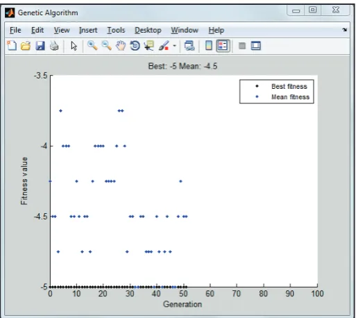
Fig. 4: Best Candidate Selection Using Genetic Algorithm
Fig. 1 shows the best candidate selection by genetic algorithm. Best
fitness values and mean fitness values are obtained. Best fitness
value is the value which is best among the current population or
it is called as the lowest fitness function.
Fig. 5: Current Best individual with Genetic Algorithm
Fig. 5 shows the current best individual with the genetic algorithm.
Average fitness value is the value which is calculated by taking the mean of all fitness values in the entire population. In each
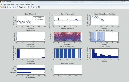
Fig. 6: Genetic Algorithm Output for Speech Recognition
Fig. 6 shows the genetic algorithm output for the speech recognisation. Figure shows the advantages of genetic algorithm in speech recognisation.
Fig. 7: Best Validation Performance Neural Network
Fig. 7 shows the best validation performance neural network for
speech recognisation. Best validation is 0.0016887 at epoch 21.
Speech recognition systems typically contain many distributions patterns. A large number of compression and other parameters are associated with speech data. This makes them both slow to decode speech, and large to store. Techniques have been proposed to decrease the number of parameters and hence increase compression of digital media.
Large vocabulary speech recognition is a computationally
expensive task with models requiring a large amount of parameters
to obtain good error rates. As we have discussed in this report that there are various techniques available for Automatic Speech recognition (ASR) namely:
Vector quantization, Neural Networks, Dynamic Time Warping, Hidden Markov Models and Genetic Algorithms and others. The main advantage of using Vector quantization in Pattern Recognition is its low computational burden when compared with other techniques such as Dynamic Time Warping and Hidden Markov Models. The main drawback when compared to Dynamic Time Warping and Hidden Markov Models is that it does not take into account the temporal evolution of the signals (speech, signature, etc.) because all the vectors are mixed up in the input Signal.
IV. Conclusion
In this work we have discussed mainly about Speech recognition and using genetic algorithms for the same. We have successfully demonstrated that genetic algorithms can be used for the automatic speech recognition in with more than 79.9% success rate. As we concluded in our results that the system we devised using genetic algorithms and neural networks produced less error rates in speaker recognition as oppose to using only one method at a time. Feature extraction is the most important part of speech recognition system. Every speech has different individual characteristics embedded in utterances. These characteristics can be extracted from a wide range of feature extraction techniques proposed and successfully exploited for speech recognition task. But extracted feature should meet some criteria while dealing with the speech signal, previous
methods have focused on ASR using LVQ, MFCC, HMM, and
ANN based approaches. In our future works we would like to improve ASR by utilizing hybrid HMM -VQ based feature
References
[1] Frikha, Mondher, Ahmed Ben Hamida,“A Comparitive
Survey of ANN and Hybrid HMM/ANN Architectures for Robust Speech Recognition.” American Journal of Intelligent
Systems 2, no. 1 (2012): 1-8.
[2] Srinivasan, A.,“Speaker identification and Verification using Vector quantization and Mel frequency Cepstral Coefficients”, Engineering and Technology 4, No. 1, pp. 33-40, 2012.
[3] Huang, Yi-bo, Qiu-yu Zhang, Zhan-ting Yuan,“Perceptual
Speech Hashing Authentication Algorithm Based on Linear Prediction Analysis”, TELKOMNIKA Indonesian Journal of Electrical Engineering 12, No. 4, pp. 3214-3223, 2014.
[4] Suni, Antti Santeri, Daniel Aalto, TuomoRaitio, PaavoAlku, MarttiVainio,“Wavelets for intonation modeling in HMM
speech synthesis”, In 8th ISCA Workshop on Speech
Synthesis, Proceedings, Barcelona, August 31-September
2, 2013.
[5] Rabiner, L. R., R. W. Schafer,“Digital Speech Processing”,
The Froehlich/Kent Encyclopedia of Telecommunications 6
(2011), pp. 237-258.
[6] Haizhou Li Bin Ma, Kong Aik Lee,“Spoken language
recognition: from fundamentals to practice”, Proceedings
of the IEEE 101, No. 5, pp. 1136-1159, 2013.
[7] Seyed Omid Sadjadi, John HL Hansen,“Unsupervised speech
activity detection using voicing measures and perceptual
spectral flux”, Signal Processing Letters, IEEE 20, No. 3, pp. 197-200, 2013.
[8] Emmanuel Vincent Jon Barker, Shinji Watanabe, Jonathan
Le Roux, Francesco Nesta, Marco Matassoni,“The second ‘CHiME’speech separation and recognition challenge:
Datasets, tasks and baselines”, In Acoustics, Speech and
Signal Processing (ICASSP), 2013 IEEE International Conference on, pp. 126-130. IEEE, 2013.
[9] M Anthimopoulos,LauroGianola, Luca Scarnato, Peter Diem,
S. Mougiakkou,“A Food Recognition System for Diabetic
Patients based on an Optimized Bag of Features Model”, 1-1, 2014.
[10] Hongbo Zhu, Tadashi Shibata,“A Real-Time
Motion-Feature-Extraction VLSI Employing Digital-Pixel-Sensor-Based Parallel Architecture”, 1-1, 2014.
[11] Mitchell M,"An Introduction to Genetic Algorithm", MIT
press Cambridge, 2005.
[12] YingjieMeng Liu, WenjunLixin Bai, Wei Chen,“Dynamic
Speech Feature Parameter Extraction Based on Fitting”, In
2014 International Conference on e-Education, e-Business and Information Management (ICEEIM 2014). Atlantis Press, 2014.
[13] KarthikaVijayan Vinay Kumar, K. Sri Rama Murty, “Feature Extraction from Analytic Phase of Speech Signals for