Performance Analysis of Distributed Computer Network over IP Protocol

(1)

International Journal of Applied Information Systems (IJAIS) – ISSN : 2249-0868 Foundation of Computer Science FCS, New York, USA

Volume 3– No.8, August 2012 – www.ijais.org

24

Performance Analysis of Distributed Computer Network

over IP Protocol

Amit Kumar Sahu

M-Tech Scholar Suresh Gyan Vihar University,

Jaipur (India)

Dinesh Goyal

HOD (Computer Science) Suresh Gyan Vihar University,

Jaipur (India)

Naveen Hemrajani

Associate Professor Suresh Gyan Vihar University,

Jaipur (India)

ABSTRACT

Computer Networking is necessary to human beings. Peoples needed to share ideas, research knowledge, and the way of life to their friends. In the modern time, the role of computer networks became dreamy. Analyzing, accessing, sharing and storing of data and information are very easy with help of distributing computer networking. Social networking sites look after human communication in a better manner and create platforms for in agreement individuals to share their thoughts and opinions. There is a massive contribution of computer networking apparatus in the progress which we see today.

This paper explores different properties for the administration for the distributed computer network environment like techniques for measuring and analyzing the performance. This analysis is precious for computer network administrator, who administrating distribute computer network.

Keywords

Networking, Traffic, Distribute computer network, Bandwidth, Delay, Reliability, Jitter.

1. INTRODUCTION

1.1Distributed computing

A field of computer science that discusses distributed systems is called Distributed computing. Multiple autonomous computers are communicates through a computer network in this system. In distributed computing, a problem is divided into many tasks, each of which is solved by one or more computers.

The platform for distributed systems has been the enterprise network linking workgroups, departments, branches, and divisions of an organization. Data is not located in one server, but in many servers. These servers might be at geographically diverse areas, connected by WAN links [1].

There are two main reasons for using distributed systems and distributed computing. First, the very nature of the application may require the use of a communication network that connects several computers. For example, data is produced in one physical location and it is needed in another location. Second, there are many cases in which the use of a single computer would be possible in principle, but the use of a distributed system is beneficial for practical reasons.

Traditionally the server had processed both the client environment and the production environment. In situations where the data could be stored on the pc itself, the processing of the production data could be executed on the local processor. But this moved the

bottleneck away from the production server processors, and to the network bandwidth [1].

1.2Measurements

The measure of computer network performance is commonly given in units of bits per second (bps). This quantity can represent either an actual data rate or a theoretical limit to available network bandwidth. Modern networks support very large numbers of bits per second. Instead of quoting 10,000 bps or 100,000 bps, networkers normally express these quantities in terms of larger quantities like "kilobits," "megabits," and "gigabits."

Measurements are conducted in four stages [2].

 Data collection

 Analysis

 Presentation

 Interpretation

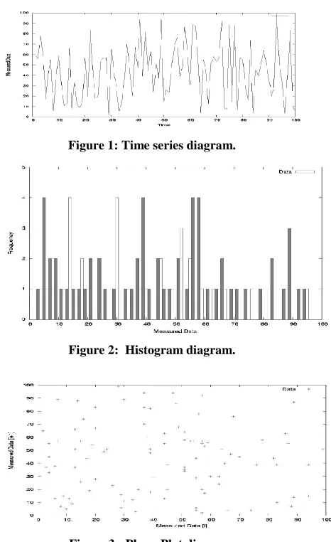
Time series

A time series diagram shows the x-axis for represent the time interval and the y-axis as the measured values of data. Time series diagrams are useful for describing the measured data, and spotting trends. An example of a time series diagram can be found in figure 1.

Histogram

A histogram is a graphical representation. It shows a visual impression of the distribution of data. In another we can say a

histogram is "a representation of a frequency distribution by means of rectangles whose widths represent class intervals and whose areas are proportional to the corresponding frequencies."

Phase plot

(2)

Figure 1: Time series diagram.

Figure 2: Histogram diagram.

Figure 3: Phase Plot diagram.

2. REVIEW of LITERATURE

2.1 Quality of Service

These days, having stable network connections is a must. With the ultimately modern world that we all live in today, a lot of our activities would no longer progress if we do not have a reliable internet connection. Communication, bank transaction, research and even shopping all depend on the worldwide web. With our extensive use of mobile phones, computers, GPS devices, music and video players, entertainment appliances and other gadgets, we certainly need to be aware of the things that we need to do to ensure that our connections are functioning well [3][4].

Quality of Service refers to a broad collection of networking technologies and techniques. The goal of Quality of Service is to provide guarantees on the ability of a network to deliver predictable results. A network monitoring system must typically be deployed as part of Quality of Service, to insure that networks are performing at the desired level [3]. The problem with a distributed computer network is that the routes may have different properties. The main properties for a distributed compute network connections are [3]:

1) Bandwidth 2) Delay 3) Reliability 4) Jitter

2.2Bandwidth

The data rate supported by a network connection or interface is known as bandwidth. Bandwidth most commonly expressed in terms of bits per second (bps). The term comes from the field of electrical engineering, where bandwidth represents the total distance or range between the highest and lowest signals on the communication channel (band)[2][3].

Table 1: Description of Bandwidth provided by various access technologies

Bandwidth is the throughput of the connection that is of interest for the customer. "Throughput is a measure of the amount of data that can be sent over network in a particulate time [4]".

The throughput is determined by the formula:

Eq-1

2.3Reliability

Reliability is term as "An attribute of any system that consistently produces the same results, preferably meeting or exceeding its specifications"[5]. It is also important to do preplanning and/or advanced preparation to provide network reliability. Of course, one way is to have additional spare capacity in the network. However, there can be a failure in the network that can actually take away the spare capacity if the network is not designed properly because of dependency between the logical network and the physical network [4].

The failure rate (λ) has been defined as "The total number of failures within an item population, divided by the total time expended by that population, during a particular measurement interval under stated conditions. It has also been defined mathematically as the probability that a failure per unit time occurs in a specified interval, which is often written in terms of the reliability function, R(t) as

Eq-2

Where t1 and t2 are the beginning and ending of a specified interval of time, and R(t) is the reliability function, i.e. probability of no failure before time t. The failure rate data can be obtained in several ways. The most common methods are [4]:

Historical data about the device or system under consideration.

Government and commercial failure rate data.

Testing.

2.4Delay

The delay of a network specifies how long it takes for a bit of data to travel across the network from one node or endpoint to another. It is typically measured in multiples or fractions of seconds. Delay may differ slightly, depending on the location of the specific pair of communicating nodes. Although only about the total delay of a network is discussed by the users. Thus, engineers usually report

Access Control Technology Bits Bytes

(3)

both the maximum and average delay and they divide the delay into several parts:

Processing delay - time taken by routers to process the packet header

Queuing delay - time spent by the packet in routing queues

Transmission delay - time taken to push the packet's bits onto the link

Propagation delay - time for a signal to reach its destination

2.5Jitter

Amount of variation in latency/response time, in milliseconds is known as Jitter. Reliable connections consistently report back the same latency over and over again. Lots of variation (or 'jitter') is an indication of problems [3]. Jitter shows up as different symptoms, depending on the application you're using. Web browsing is fairly resistant to jitter, but any kind of streaming media (voice, video, music) is quite susceptible to jitter [1]. Jitter is a symptom of other problems. It's an indicator that there might be something else wrong. Often, this 'something else' is bandwidth saturation - or not enough bandwidth to handle the traffic load [5].

3. PROPOSED WORK

In a network environment, authorized users may access data and information stored on other computers on the network. The capability of providing access to data and information on shared storage devices is an important feature of many networks. The state of a network link can be determined by measuring the throughput, the delay, the jitter and the packet loss. These four properties represent the quality of the link. In the following studies I try to measuring these properties in following section.

3.1First Study: Traffic on Network

By monitoring the network traffic for a node, information about the state of that node can be determined. This may provide the network administrator, with enough information to optimize the system performance in distributed computer system network, by removing bottlenecks. The system can represent the node, a subnet, or the whole network.

By using a passive network measurement tool, two nodes are to be monitored for one day. The data gathered from these nodes are to be analyzed, and the state of the nodes is of interest.

3.1.1Resources

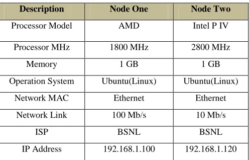
In this experiment, the resources located in table 2 have been utilized.

Table 2: Resources configuration for study one

Description Node One Node Two

Processor Model AMD Intel P IV

Processor MHz 1800 MHz 2800 MHz

Memory 1 GB 1 GB

Operation System Ubuntu(Linux) Ubuntu(Linux) Network MAC Ethernet Ethernet

Network Link 100 Mb/s 10 Mb/s

ISP BSNL BSNL

IP Address 192.168.1.100 192.168.1.120

3.1.2Tools

To perform the passive measurements, a good program for the measurements conducted in this experiment, called tcpstat. tcpstat is a highly configurable program that measures some data, and may generate some statistics if wanted. Examples of the data that can be gathered are: bits per second, bytes since last measurement, ARP packets since last measurement, TCP packets since last measurement, ICMP packets since last measurement, etc. The following command was executed on both nodes.

tcpstat -i eth0 \ -o "%S %A %C %V %I %T %U %a %d %b %p %n %N %l \n"

3.2Second Study: Throughput

By performing active measurements from one node to another node with equal link speed, the state of the connection can be determined. If the link speed is not as expected, countermeasures can be taken to locate and remove the bottleneck.

By using an active measurement tool, the connections between two nodes are to be benchmarked and analyzed. The test should provide enough information to see trends in the network, and determine if the node manage to utilize the available bandwidth. To remove uncertainties in the results, benchmarking should be executed from one node, to two other nodes.

3.2.1Resources

In this experiment, the resources are located in table 3 has been utilized.

Table 3: Resources configuration for study two

Description Node One Node Two Node Three

Processor Model

AMD Intel P IV Intel P IV

Processor MHz

1800 MHz 2800 MHz 2800 MHz

Memory 1 GB 1 GB 512 MB Operation

System

Ubuntu(Linux Based)

Ubuntu(Linux Based) Network

MAC

Ethernet Ethernet Ethernet

Network Link

100 Mb/s 100 Mb/s 100 Mb/s

ISP BSNL BSNL BSNL

IP Address 192.168.1.100 192.168.1.120 192.168.1.124

3.2.2Tools

The tool chosen to test the throughput is netperf. To execute the experiment, a server node and a client node has to be installed on each of the nodes.

For the experiment, the server program was installed on Node Two and three, and the client software was installed on Node One. This setup was chosen, so that the process of benchmarking could be controlled from Node One. This minimizes the probability for interference from each measurement.

3.3Third Study: Packet Loss, Delay and Jitter

(4)

this requires that the clocks are perfectly synchronized, an alternative method is mostly used. This is to measure the delay in form of the round trip time.

The round trip time is measured as the time it takes for one packet to be sent from a node to a destination node, until another packet is received from the destination node.

The previous cases showed methods for measuring the throughput for the link. In this last case study, the delay of a network link is to be measured, and based on those measurements; the jitter and packet loss is to be determined.

The round trip time, from one node to three other nodes are to be measured for one week. This should provide enough information to make reasonable decisions about the link state.

3.3.1Resources

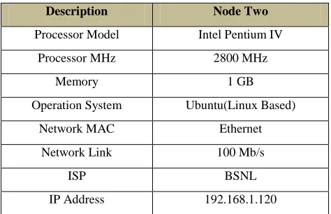
The resources utilized in this study are described in table 4.

Table 4: Resources configuration for study three

Description Node Two

Processor Model Intel Pentium IV Processor MHz 2800 MHz

Memory 1 GB

Operation System Ubuntu(Linux Based) Network MAC Ethernet

Network Link 100 Mb/s

ISP BSNL

IP Address 192.168.1.120

In addition, the link and processing power of three remote nodes has been utilized. As the active measurements does not require any installation or configuration of the destination nodes, the hardware configuration of Node Three and four are not know. The hardware configuration of Node Two can be found in table 4 (Node Two).

3.3.2Tools

The tool used to measure the data, is a modified Perl script that utilized the ping command which is available for most operating systems. The Perl script is a part of the pinger measurement package, which is used to measure round trip times from links all around the world.

The modified Perl script together with other scripts is available in the appendix.

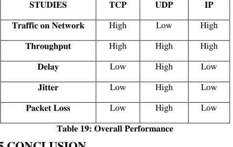
3.4Fourth Study: Overall Performance

The overall performance of a distributed computer network is shown in table 19(SECTION 4.4) using protocols Such as TCP, UDP & IP.

4. RESULTS

4.1First Study: Traffic on Network

The data collected from the two nodes by tcpstat program, consists of many lines, where each line represents one measurement. A sample from the measured data is located beneath.

Output 1

- 10 sample measurements from the tcpstat-node2.log file:

1115157729 0 0 0 117 116 1 687.73 546.39 128742.40 23.40 117 80464 0.01

1115157734 0 0 0 138 136 2 668.99 556.25 147712.00 27.60 138 92320 0.01

1115157739 0 0 0 130 122 8 674.28 540.56 140249.60 26.00 130 87656 0.01

1115157744 0 0 0 118 117 1 708.32 556.59 133731.20 23.60 118 83582 0.01

1115157749 0 0 0 126 124 2 674.03 543.12 135884.80 25.20 126 84928 0.01

1115157754 0 0 0 135 133 2 640.15 552.20 138272.00 27.00 135 86420 0.01

1115157759 0 0 0 125 121 4 701.07 545.80 140214.40 25.00 125 87634 0.01

1115157764 0 0 0 125 123 2 675.81 557.62 135161.60 25.00 125 84476 0.01

1115157769 2 0 0 120 118 2 650.70 541.93 127017.60 24.40 122 79386 0.01

1115157774 1 0 0 123 121 2 723.53 572.89 143548.80 24.80 124 89718 0.01

A description of the columns can be found in table 5.

Table 5: Description of the raw data

Column Description

Column 01 Column 02 Column 03 Column 04 Column 05 Column 06 Column 07 Column 08 Column 09

Column 10 Column 11 Column 12 Column 13 Column 14

Timestamp in UNIX time. The number of ARP packets.

The number of ICMP and ICMPv6 packets. The number of IPv6 packets.

The number of IPv4 packets. The number of TCP packets. The number of UDP packets. The average packet size.

The standard deviation of the size of each packet.

The number of bits per second. The number of packets per second. The number of packets.

The number of bytes.

The network "load" over the last minute, like in uptime.

4.1.1 Analysis and Presentation

The tcpstat program extracts some data from the host node, but it also provides some data that are processed from the measured data. These values are based on the data that has been measured since last measurement. The following values are processed by tcpstat itself, and can be viewed in the raw data log:

 The average/mean packet size.

 The standard deviation of the size of each packet.

 The number of bits per second.

 The number of packets per second.

Node One

(5)

network protocols. And it shows the load of the CPU usage, on the node.

General statistical data from the measurements of Node One can be viewed in table 6.

Table 6: Statistics for Node One

Description Bits per second Packets per

second

Minimum value Maximum value Mean value Median value Standard deviation

value

147.20 58,299,084. 80

1.266,042.45 7,160.00 6,114,076.61

0.40 28,406.80

474.57 7.40 2,555.20

The tcpstat program also measures how many transport layer packets that has passed through the system since the last measurement. Statistical data from these measurements can be viewed in table 7.

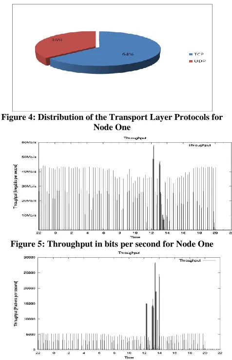
The distribution of the transport layer protocols can be viewed in the pie chart in figure 4. The transport layer protocols are TCP and UDP; these protocols are encapsulated within the IP protocol. The two first figures show the throughput, in megabits per second, for Node One. Figure 5 shows the measurement in a time series diagram and figure 6 shows the distribution of the measurements, in a histogram diagram.

Table 7: Statistics of Node One's Transport Layer Protocols

Description TCP UDP

Minimum value Maximum value Mean value Median value Standard deviation value

Sum packages Distribution of packages

0 142.022 1,507.92 9.00 10,417.22 26,056.907

63. 93%

0 75.583 850.85 14.00 7,052.29 14,702.654

36. 07%

The next two figures show the throughput, in packets per second, for Node One. Figure 7 shows the measurements in a time series diagram, while figure 8 shows the distribution of the measurements in a histogram diagram. Only the distribution from 0-50 packets per second is shown, as this represents 95.76% of the total measurements.

Figure 9 shows the CPU load of Node One at the time the measurement was conducted.

Figure 4: Distribution of the Transport Layer Protocols for Node One

Figure 5: Throughput in bits per second for Node One

Figure 6: Distribution of the throughput (bps) for Node One

Figure 7: Throughput in packets per second for Node One

(6)

Figure 9: CPU usage for Node One

Node Two

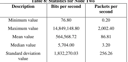
As with Node One, the same analysis and presentations has been done for Node Two. The general statistical data from the measurements of Node Two can be viewed in table 8.

Table 8: Statistics for Node Two

Description Bits per second Packets per

second

Minimum value Maximum value Mean value Median value Standard deviation

value

76.80 14,849,148.80

564,568.72 5,704.00 1,832,270.03

0.20 2,002.40

86.81 3.20 256.26

The statistical data from the transport layer packets can be viewed in table 9.

Table 9: Statistics of Node Two's Transport Layer Protocols

Description TCP UDP

Minimum value Maximum value Mean value Median value Standard deviation value

Sum packages Distribution of packages

0 10.011 429.33 7. 00 1,279.95 7,418.787

99.20%

1 2.777

3.46 2.00 28.26 59.86500

0.80% The distribution of the transport layer protocols can be viewed in the pie chart in figure 10.

Figure (figure 11) shows the CPU load of Node Two at the time the measurement was conducted.

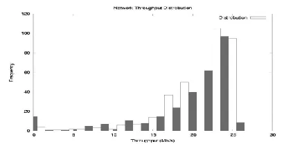
The two next figures show the throughput, in megabits per second, for Node Two. Figure 12 shows the measurement in a time series diagram and figure 13 shows the distribution of the measurements, in a histogram diagram.

The two last figures show the throughput, in packets per second, for Node Two. Figure 14 shows the measurements in a time series diagram, while figure 15 shows the distribution of the measurements in a histogram diagram.

Figure 10: Distribution of the Transport Layer Protocols for Node Two

Figure 11: CPU usage for Node Two

Figure 12: Throughput in bits per second for Node Two

Figure 13: Distribution of the throughput (bps) for Node Two

(7)

Figure 15: Distribution of the throughput (pps) for Node Two

1.1. Second Study: Throughput

The data measured between the two nodes by the netperf program, consists of many lines, where each line represents one measurement. A sample from the measured data is located beneath.

Output 2

- 10 sample measurements from the netperf-128.39.74.16.log file:

1114651931 87380 16384 16384 10.01 41.11 1114652771 87380 16384 16384 10.00 40.63 1114653732 87380 16384 16384 10.00 41.26 1114654632 87380 16384 16384 10.01 40.93 1114655532 87380 16384 16384 10.01 40.97 1114656371 87380 16384 16384 10.01 40.95 1114657332 87380 16384 16384 10.01 40.55 1114658232 87380 16384 16384 10.01 40.69 1114659132 87380 16384 16384 10.00 41.46 1114659971 87380 16384 16384 10.01 40.83 A description of the columns can be found in table 10.

Column 01 Column 02 Column 03 Column 04 Column 05 Column 06

Timestamp in UNIX time.

The buffer socket size for the receiving host. The buffer socket size for the sending host. The send size for the message.

Elapsed time, in seconds.

The throughput expressed in 106 bits per second.

1.1.1. Analysis and Presentation

The throughput of the measurements is included in the data logs, and is shown in the last column as megabits per second.

Node One to Node Two

Statistical data from the measurements between Node One and Node Two can be viewed in table 11.

A summary of the distribution of the throughput data, can be viewed in table 12. A time series graph and a histogram graph of the data are presented in figure 16 and in figure 17.

Description Value

Minimum value 0.00 Mb/s

Maximum value 25.70 Mb/s Mean value 20.20 Mb/s Median value 22.10 Mb/s

Table 11: Statistical data between Node One and Node Two

Throughput in Frequency in Percentage

00 Mb/s - 05 Mb/s 22 3% 05 Mb/s - 10 Mb/s 19 3% 10 Mb/s - 15 Mb/s 34 5% 15 Mb/s - 20 Mb/s 140 21% 20 Mb/s - 25 Mb/s 353 53% 25 Mb/s - 30 Mb/s 104 15%

Table 12: Throughput Distribution between Node One and Node Two

Figure 16: The figure shows a Throughput between Node One and Node Two

Figure 17: The figure shows the distribution of the throughput between Node One and Node Two

Node One to Node Three

Statistical data from the measurements between Node One and Node Three can be viewed in table 13.

Minimum value 0.00 Mb/s Maximum value 42.50 Mb/s

Mean value 35.40 Mb/s Median value 39.30 Mb/s

Table 13: Statistical data between Node One and Node Three

(8)

Throughput in Frequency in Percentage

00 Mb/s - 05 Mb/s 16 2% 05 Mb/s - 10 Mb/s 0 0% 10 Mb/s - 15 Mb/s 1 0% 15 Mb/s - 20 Mb/s 12 2% 20 Mb/s - 25 Mb/s 40 6% 25 Mb/s - 30 Mb/s 62 9% 30 Mb/s - 35 Mb/s 102 15% 35 Mb/s - 40 Mb/s 138 21% 40 Mb/s - 45 Mb/s 301 45% 45 Mb/s - 50 Mb/s 0 0%

Table 14: Throughput distribution between Node One and Node Three

A time series graph and a histogram graph of the data are presented in figure 18 and in figure 19.

Figure 18: The figure shows a Throughput between Node One and Node Three

Figure 19: The figure shows the distribution of the throughput between Node One

and Node Three.

1.2. Third Study: Packet Loss, Delay and

Jitter

The data collected from the three nodes by the pinger script, consists of 2.000 lines, where each line represents one measurement. A sample from the measured data is located beneath.

Output 3

- 10 sample measurements from the icmp-node4-100b-timeseries.txt file:

...

1114615202 100 10 10 185.8 187.7 190.7 - \

186.1 188.1 187.9 186.6 187.9 190.7 185.8 187.4 186.7 190.7 1114615502 100 10 10 185.7 187.3 192.0 - \

186.0 188.0 192.0 185.7 188.1 187.8 185.9 186.7 187.3 185.8 1114615802 100 10 10 185.7 189.2 203.0 - \

191.0 185.8 186.6 185.7 187.8 185.8 189.1 189.0 203.0 188.3 1114616102 100 10 10 185.8 190.1 213.3 - \

190.4 186.3 185.9 188.4 213.3 188.2 185.9 189.1 187.9 185.8 1114616402 100 10 10 185.6 188.1 192.1 - \

185.8 190.1 189.2 190.8 185.7 185.6 185.8 190.6 192.1 186.0 1114616702 100 10 10 185.7 189.6 198.8 - \

186.6 189.0 191.1 188.3 185.7 198.8 191.4 186.0 192.4 187.4 1114617002 100 10 10 185.5 189.5 199.7 - \

186.8 193.0 187.9 185.6 185.5 199.7 185.8 187.9 194.9 188.6 1114617302 100 10 10 186.0 190.7 199.6 - \

187.5 187.7 186.1 186.0 199.6 199.4 190.3 187.8 195.4 188.1 1114617602 100 10 10 185.6 189.3 200.4 - \

187.7 186.2 187.9 187.3 187.8 200.4 187.7 188.2 194.7 185.6 1114617903 100 10 10 185.7 189.1 207.9 - \

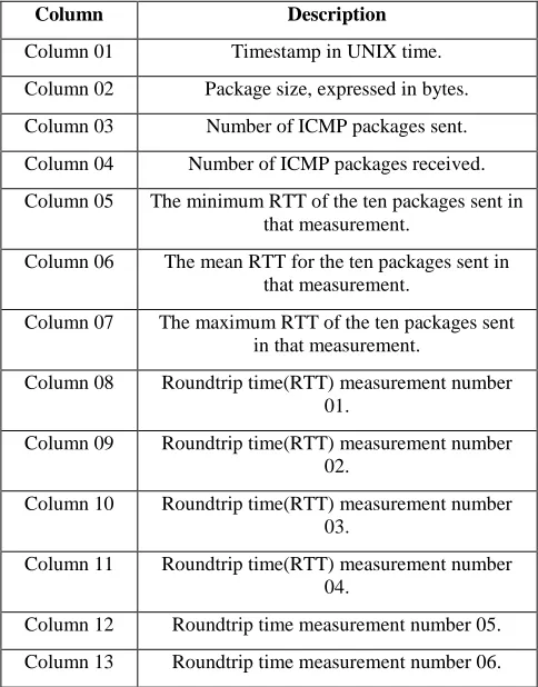
185.9 188.0 186.1 189.6 189.8 186.1 186.0 186.3 185.7 207.9 A description of the columns can be found in table 15.

Column 01 Timestamp in UNIX time. Column 02 Package size, expressed in bytes. Column 03 Number of ICMP packages sent. Column 04 Number of ICMP packages received. Column 05 The minimum RTT of the ten packages sent in

that measurement.

Column 06 The mean RTT for the ten packages sent in that measurement.

Column 07 The maximum RTT of the ten packages sent in that measurement.

Column 08 Roundtrip time(RTT) measurement number 01.

(9)

Column 14 Roundtrip time measurement number 07. Column 15 Roundtrip time measurement number 08. Column 16 Roundtrip time measurement number 09. Column 17 Roundtrip time measurement number 10.

1.2.1. Analysis and Presentation

The pinger script extracts data gathered from the active measurements, it also provides some processed data based on the measured data. The following values are processed from the ten round trip time values measured for that measurement:

 The minimum RTT of the ten packages sent in that measurement

 The mean RTT for the ten packages sent in that measurement.

 The maximum RTT of the ten packages sent in that measurement.

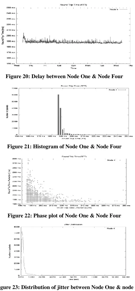
Node One to Node Four

Statistical data from the measurements between Node One and Node Three can be viewed in table 16.

Minimum value 184.70 ms Maximum value 310.30 ms Mean value 188.50 ms Median value 187.60 ms Standard deviation value 37.40 ms

Table 16: Statistical data between Node One and node four

A summary of the distribution of the round trip time data can be viewed in table 17.

Round Trip Time in Frequency in Percentage

-> 0ms 0 0%

185 ms 22 0.10%

186 ms 6041 31.20%

187 ms 2716 14.00%

188 ms 4015 20.80%

189 ms 2683 13.90%

190 ms 813 4.20%

191 ms 954 4.90%

192 ms -> 2107 10.90%

Table 17: Round Trip Time between Node 1 and Node Four

A summary of the distribution of the jitter can be viewed in table 18:

Jitter in Frequency in Percentage

0 ms 1430 7.10%

1 ms 7295 36.20%

2 ms 6178 30.70%

3 ms 1548 7.70%

4 ms 970 4.80%

5 ms -> 2738 13.60%

Table 18: Jitter between Node One and Node Four

The packet loss rate between Node One and node four, was 809/20160, as there were 809 error, and a total of 20160 packets. To present the measured and analyzed data, the following four figures are used:

Figure 20: Delay between Node One & Node Four

Figure 21: Histogram of Node One & Node Four

Figure 22: Phase plot of Node One & Node Four

Figure 23: Distribution of jitter between Node One & node four

1.3. Fourth Study: Overall Performance

(10)

STUDIES TCP UDP IP

Traffic on Network High Low High

Throughput High High High

Delay Low High Low

Jitter Low High Low

Packet Loss Low High Low

Table 19: Overall Performance

5.CONCLUSION

This paper explores different properties for the administration for the distributed computer network environment like techniques for measuring and analyzing the performance. This analysis is precious for computer network administrator, who administrating distribute computer network.

This paper includes some simple methods for analyzing and presenting the measured data, these data analysis is very useful for administrator, who maintains the distributed computer network. The three studies were expressing the functionality of the tools used to measure the four properties in quality of service.

The objective of first study is to make use of passive throughput measurement tools, to monitor the traffic on two different nodes for a particular time. In first case study the tcpstat tool successfully measured the data on nodes and provides all required information for analysis.

The objective of second study is to make use of active throughput measurement tools, to benchmark the distributed network connection between two different nodes for a particular time. The netperf tool successfully measured the throughput. In this study, the results did not match the results that predicated earlier. The mismatch generated due to limited hardware recourses.

The objective of third study is to make use of active delay measurement tools. The round trip time measurement used to find the delay and the jitter of a connection. The packet loss data can be used to figure out.

Important properties of the quality of network connection are bandwidth, delay and reliability.

6. REFERENCES

[1] William Stallings. Local networks. ACM, 1984.

[2] Mahbub Hassan and Raj Jain. High Performance TCP/IP Networking. Pearson Prentice Hall, 2004.

[3] Andrew S. Tanenbaum. Computer Networks, Fourth Edition. Prentice Hall, 2003.

[4] Lionel M. Ni Xipeng Xiao. Internet qos - a big picture. IEEE, 1999.

[5] B. Kleiner P.A. Tukey J.M. Chambers, W.S. Cleveland. Graphical Methods for Data Analysis. Duxbury Press, 1983. [6] Fred Halsall. Data Communications, Computer Networks and

Open Systems, Fourth Edition. Addison-Wesley, 1996. [7] Kevin Hamilton Kennedy Clark. Cisco LAN Switching (CCIE

Professional Development). Cisco Press, 1999.

[8] Matt Bishop. Computer Security, Art and Science. Addison-Wesley, 2002.

[9] W. Richard Stevens. The Protocols (TCP/IP Illustrated, Volume 1). Addison Wesley, 1993.

[10] Sergio Verdú. Wireless bandwidth in the making. IEEE, 2000.

[11] Annabel Z. Dodd. The Essential Guide to Telecommunications, Second Edition. Prentice Hall PTR, 1999.