Abstract— This paper proposes an experimental-based approach
to estimate the kinematic parameters and develop a cascade controller of a Cartesian robot. The aim is to satisfy the position accuracy in the trajectory execution, guaranteeing a high dynamics. The proposed procedure consists of a set of experimental tests executed on a reference trajectory, varying the velocity and acceleration in a specific range. The model is based on the Least-Square-Estimation and the Genetic Algorithms. Once the kinematic parameters have been calculated and evaluated, the controller has been built using an iterative procedure to estimate the PID gains of the position, velocity and current loops. Finally, the overall system has been validated through a set of reference trajectories, comparing the observed results with the predicted values. The RMSE index of torque has shown a congruence between the obtained results with a maximum value lower than 8.0 Nm.
Index Term— Cartesian robot, Dynamics, Cascade control,
Parameters-based model, Genetic algorithm.
I. INTRODUCTION
IN robotics applications, position accuracy and high dynamics have to be satisfied, even if these features may be conflicting [1-6]. One of the main challenge is to implement a flexible, robust and reliable control system. The development of an effective dynamic model is the successful factor to achieve a robust controller. Robot dynamics concerns with the relationship between the forces acting on a robot and the accelerations of its parts. Dynamic models may be classified in two main approaches [5]: the direct model - starting from the joint loads and knowing the joint positions-velocities, it allows to obtain the joint accelerations, and the inverse model - given the joint accelerations-velocities-positions, it defines the corresponding resultant loads acting on the joints.
The model definition is based on the use of Lagrange or Newton-Euler formulations. The advanced model-based or forces-torques control algorithms have been derived from an appropriate model selection [6]. For an optimal regulation, it is required to correctly detect and recognize the dynamic factors [3]. Nevertheless, the parameters of a robot are not always known in advance, so it is needed to apply effective procedures able of tuning the dynamic model. Usually, a conventional robot implementation procedure is composed by a set of sequential stages starting from modelling, experimental campaign and kinematic parameter optimization to fine-model tuning phase [7]. Data collection and signal processing are the critical activities to verify if the developed model reflects the
real behavior of the robot. In order to estimate the dynamic parameters, a number of techniques may be used [8, 9]. Least-Squares-Estimation (LSE) and Maximum Likelihood Estimation (MLE) approaches are most common and applied methodologies [10]. Other algorithms (e.g. Genetic-Algorithms (GAs), adaptive deep-learning techniques, data-driven methodologies) may be preferred with the intensification of data-driven methods in 4.0 era [7-11]. The mentioned methods are used to identify the optimum parameter levels of the unknown factors in the white-box configuration setting.
In this work, Authors have developed an experimental-based approach to define the appropriate kinematic model parameters of a Cartesian robot with 3 degrees of freedom (DOFs). Two techniques have been selected and evaluated: Least-Square and Genetic algorithms. In particular, the study presents the problem formulation and working principles, defining the selected algorithms used to estimate the kinematic parameters. The proposed procedure consists of executing a set of experimental tests on X-axis and Y-axis, varying the velocity and acceleration in a specific range. Then, a cascade control is presented and validated through simulations and tests, executing a number of reference trajectories.
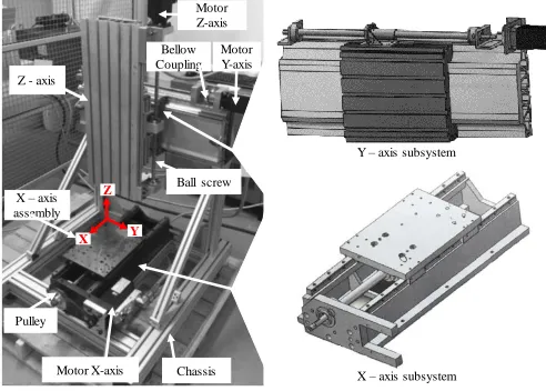
II. PROBLEM STATEMENT AND DYNAMIC MODEL This study focuses on a Cartesian robot made of modular aluminum profiles. The robot configuration presents three linear translations along the X-Y-Z axes. Figure 1 shows the reference system of the Cartesian scheme (red color). X-axis is independent while Y and Z-axes are coupled. The structure has a vertical cross configuration. The motors M1, M2, M3 provide the linear movement through endless screws, directly connected to compliant joints (Y-axis, Z-axis) or toothed belt (X-axis).
Table I summarizes the main features of each individual axis: stroke, maximum speed and acceleration.
Experimental Identification of the Dynamics
Model for Cartesian Robot
F. Aggogeri, N. Pellegrini*, F. Piaggesi and R. Adamini, Università degli Studi di Brescia, Italy
TABLEI
MAX STROKE,VELOCITY AND ACCELERATION OF THE CARTESIAN DEVICE
Symbol X-Axis Y-Axis Z-Axis
Stroke
[mm] 250.0 240.0 240.0
Velocity
[𝑚𝑚
s ]
80.0 230.0 230.0
Acceleration
[𝑚𝑚
s2]
5000.0 5000.0 5000.0
190804-5252-IJMME-IJENS © August 2019 IJENS
A. Dynamic model definition
The definition of the Cartesian dynamic model may be obtained using the Euler-Lagrange or the Newton-Euler equations. The mathematical formulation in joint-space, expressed from Lagrange equation [12], is stated by eq. (1):
𝑀(𝑞)𝑞̈ + 𝐶(𝑞, 𝑞̇)𝑞̇ + 𝜏𝑓= 𝜏 (1)
Where 𝑞(𝑡) = [𝑞1(𝑡), 𝑞2(𝑡), … , 𝑞𝑛(𝑡)]𝑇∈ ℝ𝑛is a vector of
joint (1,…,n) position. Joint velocity vector is expressed by
𝑞̇(𝑡) ∈ ℝ𝑛, and joint acceleration vector is stated by 𝑞̈(𝑡) ∈ ℝ𝑛.
The other terms correspond to the inertia matrix: 𝑀(𝑞) ∈
ℝ𝑛×𝑛
, while 𝐶(𝑞, 𝑞̇) regards Coriolis, Centrifugal and Gravitational terms, while 𝜏𝑓(𝑡) ∈ ℝ𝑛 and 𝜏(𝑡) ∈ ℝ𝑛 indicate
the friction forces and the joint torque vector, respectively. Figure 2 describes the input-output relation of each elements regarding X-axis and Y-axis.
B. Kinematic parameter estimation techniques
Authors selected two techniques to estimate the kinematic parameters of the dynamic model: “Least Squares Estimation” and “Genetic Algorithm”, processed in Matlab software. The
LSE method is an approach that uses the regression analysis to approximate the solution of overdetermined system [13]. It is a well-known method in robotics [14], and it allows the assessment of the inertial parameters obtained from the joint torques and position. The main limitation is the noise sensitivity [15]. This drawback affects the accuracy degradation in determining the kinematic parameters. To overcome this constraint, it is essential to use an identification trajectory that avoids the excitation of the robot’s dynamics. An alternative solution is the introduction of the noise filters to the sampled signals. The Genetic Algorithms (GAs) are stochastic global search formulations. GAs apply the evolutionary principle to general optimization formulations, allocating multi-search-points to working spaces and associating each search-point with appropriateness indicator according to the error of constraints-and-objective functions [16]. GAs are used in several applications from robotics to industrial and manufacturing environment [15, 17].
C. Identification of the reference trajectory
A reference trajectory has been identified and designed to evaluate the selected techniques in dynamic model development. Each axis performed a forward and backward movement with a speed equal to 20% of the maximum speed, and with an acceleration equal to 20% of the maximum permitted. Then, the same movement was executed with the same speed and acceleration increased from 40% to 80%. The procedure has been reiterated, increasing the speed to 40% and 80% of the permitted range. The scope was to excite the device dynamics, covering the maximum ranges of the possible scenarios during the robot usage. In particular, the experimental test duration (X-axis, Y-axis) was lower than 300.0 s or at least equal to 25 complete forward and reverse cycles. The torque, velocity and acceleration values have been collected and used by the algorithms in kinematic parameter estimation.
D. Kinematic parameters estimation
A preliminary analysis has been performed to evaluate the LSE algorithm applied to X-axis. By solving equations 2 and 3, the following parameters were estimated: J the equivalent inertia, c1, the coefficient of dynamic friction and c0, the coefficient of static friction.
𝑥 = Φ†𝐶
(2)
𝑥 = [ 𝐽𝑒𝑞
𝐶1
𝐶0
] , Φ = [
𝜃̈1 𝜃̇1 𝑠𝑖𝑔𝑛(𝜃̇1)
⋮ ⋮ ⋮
𝜃̈𝑡 𝜃̇𝑡 𝑠𝑖𝑔𝑛(𝜃̇𝑡)
] , 𝐶 = [
𝐶1
⋮ 𝐶𝑡
] (3)
where 𝒙 is the unknown-parameters-vector and 𝚽 is the known-values matrix (acceleration, velocity and sign of velocity). Using the column with the velocity sign, the formula has been linearized. 𝑪 is the vector of the acquired torques at each sampling time.
The GA technique has been used to identify the parameters of Y-axis. The parameters identified were: 𝑱 that is equivalent inertia, 𝒄𝟎 and𝒄𝟏, that are static and dynamic frictions, 𝒄𝒑 is a
parameter that associates the torque to the position of the axis,
Fig. 1. The Cartesian robot and X-Y Axes subsystems Bellow
Coupling Z - axis
Y – axis subsystem
X – axis assembly
Ball screw
Pulley
Chassis Motor X-axis
Motor Z-axis
Motor Y-axis
Y Z
X
X – axis subsystem
a)
b)
𝑫 is a term that includes all residues. The results are shown in Table 2.
The RMSE index has been adopted and calculated to quantify the robustness of the proposed procedure. It quantifies the error between the predicted and observed values of the torque observed on 𝑇 times. It is equal to the square root of the mean of the squares of the deviations on period T [17-21], as stated by equation (4):
𝑅𝑀𝑆𝐸 = √(∑𝑇𝑡=1(𝑦̂𝑡−𝑦𝑡)2
𝑇 ) (4)
III. THE CASCADE CONTROL LOOP
The device control has to determinate the force and torque resultants that the actuators need to provide in executing of the required trajectory. The use of a feedback loop control permits to minimize the difference between the expected values and the actual observations collected by the robot sensors.
In this way, a cascade control may be applied when the dynamics is divided in a slow part, concerning with the external loops, and a fast part, assigned to the internal loops. Each loop has the corresponding PID controller.
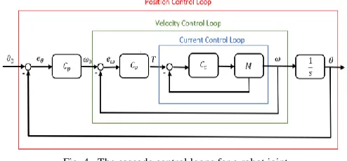
The selected configuration is based on the result of the fast dynamics of the inner loop that provides the fastest attenuation of the disturbance, minimizing potential effects on the primary output [22-25]. Three-nested PIDs have been used for position, speed and current, as shown in Figure 4. The position loop was composed by the proportional gain, P, while the speed and current loops had the proportional and integral gains, PI.
The closure of the loops was executed by the actuator, with a frequency higher than the commercial RP-1 controller. The position and speed loops had a frequency of 2.0k Hz, the current loop had a frequency of 8.0k Hz, while the frequency of the RP-1 controller was 500 Hz. The current loop was the most inner and fastest loop, with a sampling rate of 8.0 kHz.
Ad-hoc tuning phase was performed to establish the current loop gains, by setting the position and velocity values gains as described in Table 3. Three main scenarios has been considered and compared. This approach is modular and valid for additional cases.
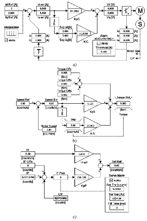
The current loop gains have been defined when the obtained torque value differed from the expected torque parameter of 5% - 10%. At first, a proportional gain was set equal to 0.02 while the integral gain was equal to zero. Then, the proportional gain has been increased by 50% every time, until the current loop was unstable. The PID gains were progressively reduced by 10%, until the oscillation disappeared. This operation has been repeated for the other PID gains. Figure 5(a) describes the scheme of the current loop.
The velocity loop on the drive was controlled by a PI scheme with proportional and integral actions. It was the second inner loop, with a sampling rate of 2.0 kHz. The velocity loop has been tuned executing the proposed procedure with the motor free to rotate. Then, the motor has been connected to the robot, the proportional and integral gains have been refined with an iterative procedure. In this phase, a velocity square wave with the reference value changing from 0% to 10% of the maximum value of the speed parameter was used. Figure 5(b) shows the scheme of the velocity loop.
The position loop on the drive was managed by a P controller, the proportional gain. It was the third loop, with a sampling rate of 2.0 kHz. The motor has been connected to the robot and the proportional gain “KpP” was increased up to
unstable condition of “Epos” position loop feedback [26]. Figure 5(c) shows the control scheme of the position loop. TABLEII
KINEMATIC PARAMETER ESTIMATION
Symbol Description X-Axis Y-Axis
ET Estimation
Technique Least Square
Genetic Algorithm
J [kgm2] Equivalent
Inertia 0.000089 0.000100
c0 [Nm] Coefficient of static friction 0.2198 0.3230
c1[
kgm2
s ]
Coefficient of
dynamic friction 0.000312 0.000500
cp [Nm]
Parameter that correlate the Torque
and Axis position
- 0.000500
D [Nm] Residuals term - 0.006200
RMSE [Nm] Root Mean Square
Error 7.993 3.799
Fig. 4. The cascade control loops for a robot joint
TABLEIII
PIDGAINS ESTIMATION FOR CASCADE CONTROL
Scenario Loop Gain Value
1 Position FwF 1.00
1 KpP 150.00
1 Velocity KpS 0.12
1 KiS 20.00
2 Position FwF 0.50
2 KpP 170.00
2 Velocity KpS 0.17
2 KiS 15.00
3 Position FwF 1.00
3 KpP 200.00
3 Velocity KpS 0.30
190804-5252-IJMME-IJENS © August 2019 IJENS A validation campaign has been executed to verify if the
estimated parameters were correctly aligned with the parameters obtained by the experimental tests. Figure 6 shows a comparison between the PID gain scenarios for X-axis defined in Table 3.
Figure 6(a) states the reference trajectory used to validate the gain parameters while Figure 6(b) highlights the deviations between Scenario 1 and Scenario 3 related to velocity [rad/s]. The oscillating case is the configuration with the highest value of integral gain (blue curve). The optimal parameter setting is Scenario 3 (black color), that shows the fastest response without perturbations at 10.0 s and 27.0 s – 30.0 s (critical periods). Figure 6(c) presents the torque analysis. The optimal parameter configuration is shown by Scenario 3, that minimizes the perturbations in critical periods.
IV. EXPERIMENTAL CAMPAIGN VALIDATION
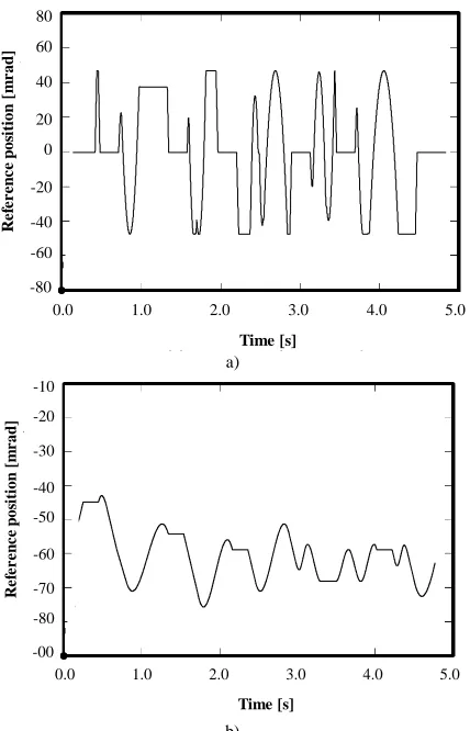
The validation of the overall system has been verified executing a set of trajectories and comparing the measured torques with the estimated values. Figure 7 describes an example related to a reference trajectory executed on X-Y-axes, respectively. The aim was to reproduce a standard robot task in working space and conditions.
The results show that the RMSE error between the predicted torques and the measured torques is lower than 8.0 Nm, confirming the robustness of the proposed approach.
In particular, Figure 8 (a-b) presents a comparison between the observed and estimated values of acceleration and torque related to Y-axis using the GA techniques. The RMSE index, calculated on the validation model, has a value equal to 4.78 Nm. In the same way, Figure 8 (c-d) shows the comparison between the accelerations and torques applying the LSE estimated parameters.
The value of RMSE is equal to 7.99 Nm. This deviation is due to the torque signal noise.
a)
b)
c)
Fig. 5. The current loop (a), velocity loop (b) and position loop (c).
a)
b)
c)
Fig. 6. The predefined reference trajectory (a), X-axis velocity comparison between scenarios 1-3 (b) and X-axis torque comparison between scenarios
1-3 (c) -1.0
-2.0
-3.0
-4.0
-5.0
-6.0
-7.0
-8.0
-9.0
C
u
r
r
e
n
t p
os
iti
on
[r
ad
]
Time [s]
0.0 10.0 20.0 30.0 40.0 50.0
-70 -60 -50 -40 -30 -20 -10 0
1
1529 4357 7185 99113 127141 155169 183197 211225 239253 267281 295309 323337 351 365379 393407 421435 449463 477491 505519 533547 561575 589603 617631 645659 673687
Position
Serie1
80
60
40
20
0
-20
-40
-60
-80
C
u
r
r
e
n
t v
e
loc
ity
[r
ad
/s
]
Time [s]
0.0 10.0 20.0 30.0 40.0 50.0
-60 -40 -20 0 20 40 60
Differenza Vel
Serie1 Serie2 Serie3
Scenario 1 Scenario 2 Scenario 3
4.0
3.0
2.0
1.0
0.0
-1.0
-2.0
-3.0
-4.0
T
or
q
u
e
[N
m
]
Time [s]
0.0 10.0 20.0 30.0 40.0 50.0
-3 -2 -1 0 1 2 3 4
Differenza coppie PID
Serie1 Serie2 Serie3
This result may be considered acceptable since the noise generated by the static friction has not been evaluated in the preliminary test.
V. CONCLUSION
One of the most critical task of a robot is to satisfy the required trajectory accuracy guaranteeing a high dynamics. In this study, an experimental-based approach to estimate the kinematic parameters of a Cartesian robot is presented. The proposed procedure consisted on a set of experimental tests executed on a defined trajectory. The aim is to excite the device dynamics, covering the maximum ranges of the possible scenarios during the robot usage. The dynamic model focuses on the Least-Square-Estimation and the Genetic Algorithms. Based on the calculated kinematic parameters, the cascade controller has been developed by a sequential procedure to estimate the PID gains of the position, velocity and current loops. Finally, the controlled Cartesian robot performance has been confirmed through a set of predefined reference trajectories, comparing the observed results with the expected values. For a practical implementation, the RMSE index has shown a congruence of the obtained results with a maximum value lower than 8.0 Nm, equal to 4.78 Nm and 7.99 Nm for GAs and LSE, respectively. Further works could investigate the torque signal noise monitoring, the extension of kinematic parameter identification techniques (in addition to LSE and GAs) and the inclusion of vertical axis in the robot dynamic model.
a)
b)
c)
d)
Fig. 8. The comparison between the observed and estimated accelerations (a) and torque (b) (Y-axis – Genetic Algorithm) – accelerations (c) and
2.0 1.5 1.0 0.5 0 -0.5 -1.0 -1.5 -2.0 A c c e le r ati on [r ad /s 2] Time [s]
0.0 1.0 2.0 3.0 4.0 5.0
-2000 -1500 -1000 -500 0 500 1000 1500 2000 Acc. Estimated Acc. Measured
2.0 1.5 1.0 0.5 0 -0.5 -1.0 -1.5 -2.0 T or q u e [N m ] Time [s]
0.0 1.0 2.0 3.0 4.0 5.0
Torque Estimated Torque Measured
-1.5 -1 -0.5 0 0.5 1 1.5 4.0 3.0 2.0 1.0 0 -1.0 -2.0 -3.0 -4.0 A c c e le r ati on [r ad /s 2] Time [s]
0.0 1.0 2.0 3.0 4.0 5.0
Acc. Estimated -5000 -4000 -3000 -2000 -1000 0 1000 2000 3000 4000
5000 Acc. Measured
2.0 1.5 1.0 0.5 0 -0.5 -1.0 -1.5 -2.0 T or q u e [N m ] Time [s]
0.0 1.0 2.0 3.0 4.0 5.0
-1.5 -1 -0.5 0 0.5 1 1.5
Torque Estimated Torque Measured a)
b)
Fig. 7. The reference position for the trajectory on Y-axis (a), and X-axis (b). 80 60 40 20 0 -20 -40 -60 -80 R e fe r e n c e p os iti on [ m r ad ] Time [s]
0.0 1.0 2.0 3.0 4.0 5.0
-60 -40 -20 0 20 40 60 AXE:IV(2) -10 -20 -30 -40 -50 -60 -70 -80 -00 R e fe r e n c e p os iti on [m r ad ] Time [s]
0.0 1.0 2.0 3.0 4.0 5.0
190804-5252-IJMME-IJENS © August 2019 IJENS REFERENCES
[1] W. P. Risk, G. S. Kino, and H. J. Shaw, “Fiber-optic frequency shifter using a surface acoustic wave incident at an oblique angle,” Opt. Lett., vol. 11, no. 2, pp. 115–117, Feb. 1986.
[2] D. B. Payne and J. R. Stern, “Wavelength-switched pas- sively coupled single-mode optical network,” in Proc. IOOC-ECOC, Boston, MA, USA, 1985, pp. 585–590.
[3] A. Beiranvand, A. Kalhor, M. Tale Masouleh, “An Exprrimental Modelling and Identification of Free Drive Dynamics with Considering Variable Friction”, International Conference on Robotics and Mechatronics (IcRoM 2018), october 23-25 2018, Tehran, Iran.
[4] Roy B, Asada H, “Nonlinear feedback control of a gravity-assisted under actuated manipulator with application to aircraft assembly”, IEEE Trans Robot 2009, 25:1125-33.
[5] G. Legnagni, Robotica Industriale, Casa Editrice Ambrosiana, (2003) [6] Wu J, Wang J, You Z, “An overview of dynamic parameter identification
of robots”, Robot Comput Integr Manuf 2010;26:414-9.
[7] Swevers J, Verdonck W, Schutter J. “Dynamic model identification for industrial robots”, IEE Control System Magazine, 2007;27(5):58-71 [8] Gautier M, Halil W, Restrepo P, “Identification of the dynamic parameters
of a close loop robot”, International conference on robotics and automation, p. 3045-50.
[9] M. Sayahkarajy and Z. Mohamed, “Mixed Sensitivity H 2 / H ∞ Control of a Flexible-Link Robotic Arm,” Int. J. Mech. Mechatronics Eng. IJMME-IJENS, vol:14, no. 1, pp. 21–27, 2014.
[10]Jin J, Gans N, “Parameter identification for industrial robots with a fast and robust trajectory design approach”, Robotic and Computer-Integrated Manufacturing, 31 (2015) 21-29.
[11] F. Salem, A. Michel, A. Ziad, “Mechatronics engineering implementation of multilevel control of a complex hybrid robot,” Int. J. Mech. Mechatronics Eng. IJMME-IJENS, vol: 18, no.2, pp. 53-63, 2018. [12]A. Jaritz MW Spong. “Parameter identification of industrial robot” [13]B. Siciliano, L. Sciavicco, L. Villani, G. Oriolo, Robotica. “Modellistica,
pianifcazione e controllo”, McGraw-Hill, 2008
[14] Gautier M, Khalil W. “Direct calculation of minimum inertial parameters of serial robots”. IEEE Transaction on Robotics and Automation 1990; 6(3): 368-73
[15] K. Fujita, N. Hirokawa, S. Akagi, S. Kitamura, H. Yokohata, “Multi-objective optimal design of automotive engine using genetic algorithm”, 1998 ASME Design Engineering Technical Conferences, September 13 -16, 1998, Atlanta, Georgia
[16] G. Shin, Y. Song, T. Lee, H. Choi (2007), “Genetic Algorithm for Identification of Time Delay Systems from Step Responses”, in: International Journal of Control, Automation, and Systems, Vol 5, no. 1, pp. 79-85
[17] J.-S. Chiou, M.-T. Liu, “Using fuzzy logic controller and evolutionary genetic algorithm for automotive active suspension system”, International Journal of Automotive Technology, Springer, 12/2009, 10:703
[18] K. Kozlowski “Modelling and identification in robotics”. New York: Springer-Verlag; (1998).
[19] K. Kelley, K. Lai, “Accuracy in Parameter Estimation for the Root Mean Square Error of Approximation: Sample Size Planning for Narrow Confidence Intervals”, Multivariate Behavioral Research, 46:132, (2011). [20] V. Parra Vega, S. Arimoto, Y.H. Liu, G. Hirzinger, P. Akella, Dynamic sliding PID control for tracking of robot manipulators: theory and experiments, IEEE Trans. Robot. Autom. 19 (6) (2003) 967–976. [21] H. Taghirad, Parallel Robots Mechanics And Control, Taylor & Francis,
CRC Press, 2013.
[22] O. Arrieta, R. Vilanova, P. Balaguer (2008), Procedure for Cascade Control Systems Design, in: "Int. J. of Computers Communications & Control" vol. III, No. 3, pp. 235-248
[23]C.C. Cheah, S. Kawamura, S. Arimoto, Feedback Control For Robotic Manipulator With an Uncertain Jacobian Matrix, Adv. Robot Kinematics: Motion Man Machin J. Robot. Syst. 16 (2) (1999) 119–134
[24] S. Radhakrishnan, W. Gueaieb, Genetic algorithm based direction finder on the manifold for singularity free paths, 2016 IEEE International Symposium on Robotics and Intelligent Sensors (IRIS) (2016) 151–156, [25] Yang, G.J. , Delgado, R. , Choi, B.W. , 2016. A practical joint-space
trajectory generation method based on convolution in real-time control. Int. J. Adv. Robot. Syst. 13 .
[26] Lu, B. , Wu, X. , Figueroa, H. , Monti, A. , 2007. A low-cost real-time hard- ware-in-the-loop testing approach of power electronics controls. IEEE Trans. Ind. Electron. 54, 919–931.
Francesco Aggogeri is an Associate Professor of
Applied Mechanics at University of Brescia. His main research interests include Applied Mechanics, Robotics, Mechatronic Devices, Rehabilitation Engineering and Vibration control. He is the author of a number of papers (ISI-Scopus) and peer-review conference proceedings papers. Francesco Aggogeri is responsible of national and international research projects. He is the unit coordinator of PROGRAMS (H2020 project) and he has served as responsible of IntegMicro FP7 project) and Copernico (EU-FP7 project).
Nicola Pellegrini is an Assistant Professor of Applied
Mechanics at University of Brescia. He has been involved in projects related to integrated mechatronic systems, Product development, Motion planning and Soft computing simulation. He is author of a number of papers published in international journals and conferences. He has collaborated to National and European research programs and projects funded by private companies.
Filippo Piaggesi received the B.S. degree in
Automation engineering from University of Brescia, Italy, in 2016 and the M.S. degree in automation engineering from University of Brescia, Italy, in 2018. He is currently collaborating with Mechanical and Industrial department of University of Brescia. His research interest focuses on the development of Cartesian Robot dynamic models and the application of algorithms for the estimation of dynamic parameters.
Riccardo Adamini is currently a Full Professor of