e-ISSN: 2278-067X, p-ISSN: 2278-800X, www.ijerd.com Volume 7, Issue 4 (May 2013), PP. 47-54
Data Classification with Genetic Programming (Gp) – A
Case Study
N.Prasanna Kumari,
Assistant Professor, Dept of CSE AITAM Tekkali, Andhra Pradesh, INDIA.
Abstract:- Classification is one of the most researched questions in data mining. A wide range of real problems have been stated as classification problems, for example credit scoring, bankruptcy prediction, medical diagnosis, pattern recognition, text categorization, software quality assessment, and many more. The use of evolutionary algorithms for training classifiers has been studied in the past few decades. Genetic programming is a technique to automatically discover computer programs using principles of evolution. Genetic operations like crossover, mutation, reproduction are carried out on population to get the best fitting results. In this GP is used for developing a classification model for a data set and also used for function generation to study its automatic code generation capability.
Keywords:- Classification, data mining, Genetic Programming;
I. INTRODUCTION
Classification is the data mining problem of attempting to predict the category of categorical, numerical or mixed data by building a model based on some predictor variables. Classification is much easier to understand. First, we define a set of groups by their characteristics. Then we analyze each case and put it into the group it belongs. Classification can be used to understand the existing data and to predict how new instances will behave. For example, we can make a classification model for a Haberman’s survival data to find out hidden patterns and predictions. First we define two patient groups: one is for the patients who survive for 5years or longer; the other group is the patients who will die within 5 years[1-5].
The genetic algorithm is a probabilistic search algorithm that iteratively transforms a set (called a population) of mathematical objects (typically fixed-length binary character strings), each with an associated fitness value, into a new population of offspring objects using the Darwinian principle of natural selection and using operations that are patterned after naturally occurring genetic operations, such as crossover (sexual recombination) and mutation[1-5].
Genetic programming (GP) is a branch of genetic algorithms. GP applies the approach of the genetic algorithm to the space of possible computer programs. GP is a technique to automatically discover computer programs using principles of Darwinian evolution. In this thesis GP is used as a problem-solving tool for solving few mathematical equations, further it used as classifier. It is a systematic method for getting computers to automatically solve a problem starting from a high-level statement of what needs to be done. IT is a domain-independent method that genetically breeds a population of computer programs to solve a problem. It iteratively transforms a population of computer programs into a new generation of programs by applying analogs of naturally occurring genetic operations[1-5].
The present work is mainly concentrated on data classification using genetic programming, which gives a mathematical model to classify a two class modeled data to produce nearest genetic programming classifier expression, which gives a best data classification percentage.
A. Scope of Study
•Study about Genetic programming and Genetic Algorithm.
•Study Genetic Algorithm for generating a polynomial equivalent to the given polynomial. •Study about the Classification problem of Data Mining.
•Study how we can use Genetic Programming for solving the Classification problem. •Select any data set on which the GP has to be applied.
B. Objectives of the Study
•The purpose of the software is to classify a data set.
II. BACKGROUNDINFORMATION A. Classification
Data classification is the categorization of data for its most effective and efficient use. In a basic approach to storing computer data, data can be classified according to its critical value or how often it needs to be accessed, with the most critical or often-used data stored on the fastest media while other data can be stored on slower (and less expensive) media[6-13]. Classification Examples
Classifying credit card transactions as legitimate or fraudulent.
Classifying secondary structures of protein as alpha-helix, beta-sheet, or random coil. Categorizing news stories as finance, weather, entertainment, sports, etc.
B. Classification Methods Decision Tree Induction Neural Networks Bayesian Classification
Association-based Classification K-Nearest Neighbor
Case-Based Reasoning Genetic Algorithms Fuzzy Sets
i. Bayesian Classification
Is based on the so-called Bayesian theorem and is particularly suited when the dimensionality of the inputs is high [14].
Fig 1 Distribution of two different colored objects to explain Bayesian Classification
The objects can be classified as either GREEN or RED shown in Fig 1. Our task is to classify new cases as they arrive, i.e., decide to which class label they belong, based on the currently existing objects. Since there are twice as many GREEN objects as RED, it is reasonable to believe that a new case (which hasn’t been observed yet) is twice as likely to have membership GREEN rather than RED[6-14].
In the Bayesian analysis, this belief is known as the prior probability. Prior probabilities are based on previous experience, in this case the percentage of GREEN and RED objects, and often used to predict outcomes before they actually happen.
Prior Probability for GREEN ∞ Number of GREEN objects Total number of objects Prior Probability for RED ∞ Number of RED objects Total number of objects Likelihood of X given GREEN ∞ 40/60
Likelihood of X given RED ∞ 20/60
ii. Decision Tree Induction
A decision tree is a flow chart like structure in which the internal nodes represent tests on an attribute, each branch represents the outcome of the test, and each leaf node represents a class label. The attribute with the maximum value of information gain is selected as the root node. Decision tree generation consists of two phases[6-14].
Tree construction:
At start, all the training examples are at the root.
Partition examples recursively based on selected attributes. Tree pruning:
iii. Neural Networks
Neural networks are a form of multiprocessor computer system, with Simple processing elements
A high degree of interconnection Simple scalar messages
Adaptive interaction between elements
A typical neural network is composed of input units X1, X2, ... corresponding to independent variables (in our
case, highway or intersection variables), a hidden layer known as the first layer, and an output layer (second layer) whose output units Y1, ... correspond to dependent variables (expected number of accidents per time
period). In between are hidden units H1, H2, ... corresponding to intermediate variables. These interact by means
of weight matrices W(1) and W(2) with adjustable weights [6-14]
III. GENETICALGORITHMANDPROGRAMMING
Genetic Programming is a technique to automatically discover computer programs using principles of Darwinian evolution. In this thesis GP is used as a problem-solving tool for solving few mathematical equations, further it used as classifier. Genetic Programming (GP) is a systematic method for getting computers to automatically solve a problem starting from a high-level statement of what needs to be done[15-22].
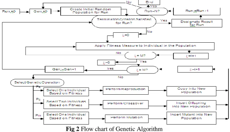
Fig 2 Flow chart of Genetic Algorithm
IT is a domain-independent method that genetically breeds a population of computer programs to solve a problem. It iteratively transforms a population of computer programs into a new generation of programs by applying analogs of naturally occurring genetic operations.
A. Genetic Algorithm
The genetic algorithm is a probabilistic search algorithm that iteratively transforms a set (called a population) of mathematical objects (typically fixed-length binary character strings), each with an associated fitness value, into a new population of offspring objects using the Darwinian principle of natural selection and using operations that are patterned after naturally occurring genetic operations, such as crossover (sexual recombination) and mutation[15-23].
i. Description: A typical genetic algorithm requires two things to be defined:
A genetic representation of the solution domain. A fitness function to evaluate the solution domain.
Once we have the genetic representation and the fitness function defined, GA proceeds to initialize a population of solutions randomly, then improve it through repetitive application of mutation, crossover, inversion and selection operators [15-24].
ii. Initialization
space). Occasionally, the solutions may be "seeded" in areas where optimal solutions are likely to be found[15-24].
iii. Selection
During each successive generation, a proportion of the existing population is selected to breed a new generation. Individual solutions are selected through a fitness-based process, where fitter solutions (as measured by a fitness function) are typically more likely to be selected. Certain selection methods rate the fitness of each solution and preferentially select the best solutions. Other methods rate only a random sample of the population, as this process may be very time-consuming.
Most functions are stochastic and designed so that a small proportion of less fit solutions are selected. This helps keep the diversity of the population large, preventing premature convergence on poor solutions. Popular and well-studied selection methods include roulette wheel selection and tournament selection[15-24].
iv. Reproduction
The next step is to generate a second generation population of solutions from those selected through genetic operators: crossover (also called recombination), and/or mutation. For each new solution to be produced, a pair of "parent" solutions is selected for breeding from the pool selected previously. By producing a "child" solution using the above methods of crossover and mutation, a new solution is created which typically shares many of the characteristics of its "parents". New parents are selected for each child, and the process continues until a new population of solutions of appropriate size is generated [15-24].
These processes ultimately result in the next generation population of chromosomes that is different from the initial generation. Generally the average fitness will have increased by this procedure for the population, since only the best organisms from the first generation are selected for breeding, along with a small proportion of less fit solutions, for reasons already mentioned above.
v. Termination
This generational process is repeated until a termination condition has been reached. Common terminating conditions are
A solution is found that satisfies minimum criteria Fixed number of generations reached
Allocated budget (computation time/money) reached
The highest ranking solution's fitness is reaching or has reached a plateau such that successive iterations no longer produce better results
Manual inspection
Combinations of the above
vi. Applications of Genetic Algorithm
Distributed computer network topologies.
Code-breaking, using the GA to search large solution spaces of ciphers for the one correct decryption.
File allocation for a distributed system. Finding hardware bugs.
Software engineering
Learning Robot behavior using Genetic Algorithms
B. Genetic Programming
Genetic programming is a branch of genetic algorithms. GP applies the approach of the genetic algorithm to the space of possible computer programs. The main difference between genetic programming and genetic algorithms is the representation of the solution. Genetic programming creates computer programs in the lisp or scheme computer languages as the solution. Genetic algorithms create a string of numbers that represent the solution[15-24]. Compared with genetic algorithms (GAs), GP has the following characteristics:
While the standard genetic algorithms (GAs) use strings to represent solutions, the forms evolved by genetic programming are tree-like computer programs. The standard GA bit strings use a fixed length representation while the GP tree-like programs can vary in length.
While GAs need a very complex encoding and decoding process, GP eliminates this process by directly using terminals and functions and accordingly GP is easier to use.
The term genetic programming comes from the notion that computer programs can be represented by a tree-structured genome. Computer programming languages, such as Lisp, can be represented by formal grammars which are tree based, thus it is actually relatively straight forward to represent program code directly as trees. These trees are randomly constructed from a set of primitive functions and terminals[15-24].
i. Why Genetic Programming is used
No analytical knowledge is needed and we can still get accurate results.
Every component of the resulting GP rule-base is relevant in some way for the solution of the problem. Thus we do not encode null operations that will expend computational resources at runtime.
This approach does scale with the problem size. Some other approaches to the cart centering problem use a GA that encodes NxN matrices of parameters. These solutions work bad as the problem grows in size (i.e. as N increases).
With GP we do not impose restrictions on how the structure of solutions should be. Also we do not bind the complexity or the number of rules of the computed solution.
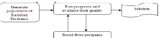
ii. Main Loop of Genetic Programming
Fig 3 Main loop of genetic programming
Genetic programming starts by creating a random population of syntactic trees. A new generation or population is evolved from this initial random population[15-24]. The members of the new population (or generation) are the members of the initial population that satisfied the fitness of the problem in question. After selection, the genetic operations are implemented on the new population which gives rise to another new population. Again fitness criteria are applied on the new population and genetic operations will be applied on those that have satisfied the fitness. This is an iterative process which is performed until the desired solution is obtained. Figure 3 shows the idea.
iii. Uses of Genetic Programming
GP-based techniques are distribution free, i.e no prior knowledge is needed about statistical distribution of data.
Expresses relation between the attributes mathematically.
Automatic code generator.
The source code for one classification problem can be easily mapped for another problem.IV. CASESTUDY
i. Fitness Measure
GP is guided by the fitness function to search for the most efficient computer program to solve a given problem. A simple measure of fitness has been adopted for the pattern classification problem.
Fitness = Number of samples classified correctly Number of samples used for training during evolution
ii. Creation of Training Sets
valid training set for a two-class problem, still it results in a highly skewed training set as there are more representative samples for one category than for the other. Our experimental results show that this skew ness leads to misclassification of input feature vectors. To overcome the skew ness, one possible option is to use a subset of the data belonging to other classes (whose desired output is -1), so that the number of samples belonging to a class will be the same as the number of samples belonging to other classes. Although a balanced training set is created in this manner, it will lead to poor learning as the data for the other classes are not representative. The training set should be as representative as possible for proper learning of underlying data relationships. So, an interleaved data format for the training set is used to evaluate the fitness function.
iii. Interleaved Data Format
In the interleaved data format, the samples belonging to the true class are alternately placed between samples belonging to other classes, i.e., they are repeated. The table below illustrates the format of the training set for class 1 in a five-class problem. The desired output of the GPCE is 1 for the samples of the true-class, and is -1 for the other classes [25]. The number of samples in the training set is increased, and hence the time taken for evaluating fitness also increases. The training time is proportional to the size of the training set. Hence, the training time for evolving the GPCE of class 1 with the skewed data set is proportional to n1+N1, and for the
interleaved data format, it is proportional to (n-1)n1+N1. Interleaved data format training set of GPCE-1 in a
five-class problem
Class#1, n1(+1), n2(-1), n1(+1), n3(-1), n1(+1), n4 (-1), n1 (+1), 5 (-1)
iv. Data Set Description for Data Classification
Haberman’s Survival Data Set
In this thesis, GP is applied to Haberman’s survival data set. Dataset contains cases from study conducted on the survival of patients who had undergone surgery for breast cancer [8] [9].
Table 1 Haberman`s Survival Data Set
v. Data Set Information:
The dataset contains cases from a study that was conducted between 1958 and 1970 at the University of Chicago's Billings Hospital on the survival of patients who had undergone surgery for breast cancer.
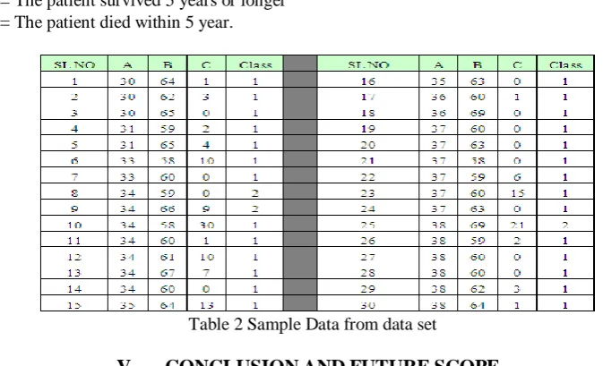
vi. Attribute Information:
Age of patient at time of operation (numerical) Patient's year of operation (year - 1900, numerical) Number of positive auxiliary nodes detected (numerical) Survival status (class attribute)
1 = The patient survived 5 years or longer 2 = The patient died within 5 year.
Table 2 Sample Data from data set
V. CONCLUSIONANDFUTURESCOPE
works reviewed, and serves as a guideline to categorize and sort relevant literature. In this study we classify the data for the Haberman’s data set. In this we consider single category classification; This can be enhanced further for Multi category classification problems as a class problem should be solved as n-two class problems
REFERENCES
[1]. R. Aler, D. Borrajo, and P. Isasi, “Using Genetic Programming to learn and improve control knowledge,” Artif. Intell., vol. 141, no. 1–2, pp.29–56, Oct. 2002.
[2]. H. Forrest, J. R. Koza, Y. Jessen, and M.William, “Automatic synthesis,placement and routing of an amplifier circuit by means of genetic programming,”in Lecture Notes in Computer Science, vol. 1801,Evolvable Systems: From Biology to Hardware, Proc. 3rd Int. Conf.(ICES), pp. 1–10, 2001. [3]. J. K. Kishore, L. M. Patnaik, V. Mani, and V. K. Agrawal, “Application of genetic programming for
multicategory pattern classification,” IEEE Trans. Evol. Comput., vol. 4, pp. 242–258, Sept. 2000. [4]. P. J. Rauss, J. M. Daida, and S. Chaudhary, “Classification of spectral imagery using genetic
programming,” in Proc. Genetic Evolutionary Computation Conf., pp. 733–726, 2000.
[5]. D. Agnelli, A. Bollini, and L. Lombardi, “Image classification: an evolutionary approach,” Pattern Recognit. Lett., vol. 23, pp. 303–309, 2002.
[6]. T.-S. Lim, W.-Y. Loh, and Y.-S. Shih, “A comparison of prediction accuracy, complexity and training time of thirty-three old and new classification algorithms,” Mach. Learning J., vol. 40, pp. 203–228, 2000.
[7]. D. E. Goldberg, Genetic Algorithm in Search, Optimization and Machine Learning. Reading, MA: Addison-Wesley, 1989.
[8]. J. Eggermont, J. N. Kok, and W. A. Kosters. Genetic programming for data classification: partitioning the search space. In Proceedings of the 2004 ACM symposium on Applied computing, SAC ’04, pages 1001–1005, New York, NY, USA,2004.
[9]. A. S. Kumar, S. Chowdhury, and K. L. Mazumder, “Combination of neural and statistical approaches for classifying space-borne multispectral data,” in Proc. ICAPRDT, Calcutta, India, pp. 87–91, 1999. [10]. T M Khoshgoftaar and E B Allen A practical classification rule for software quality models IEEE
Transactions on Reliability, 49(2),2000.
[11]. Tsakonas, A, A comparison of classification accuracy of four genetic programming-evolved intelligent structures, Information Sciences, pp. 691-724, . 2006
[12]. T. K. Ho and M. Basu. Complexity measures of supervised classification problems. IEEE Trans. Pattern Anal. Mach. Intell., 24:289–300, 2002.
[13]. I. De Falco, A. Della Cioppa, and E. Tarantino, “Discovering interesting classification rules with genetic programming,” Appl. Soft Comput., vol. 23, pp. 1–13, 2002.
[14]. A. I. Esparcia-Alcazar and K. Sharman, “Evolving recurrent neural network architectures by genetic programming,” in Proc. 2nd Annu. Conf. Genetic Programming, pp. 89–94, 1997.
[15]. G. Dounias, A. Tsakonas, J. Jantzen, H. Axer, B. Bjerregaard, and D. Keyserlingk, “Genetic programming for the generation of crisp and fuzzy rule bases in classification and diagnosis of medical data,” in Proc. 1st Int. NAISO Congr. Neuro Fuzzy Technologies, Canada, 2002.
[16]. C. C. Bojarczuk, H. S. Lopes, and A. A. Freitas, “Genetic Programming for knowledge discovery in chest pain diagnosis,” IEEE Eng.Med. Mag., vol. 19, no. 4, pp. 38–44, 2000.
[17]. T. Loveard and V. Ciesielski, “Representing classification problems in genetic programming,” in Proc. Congr. Evolutionary Computation pp. 1070–1077, 2001.
[18]. B.-C. Chien, J. Y. Lin, and T.-P. Hong, “Learning discriminant functions with fuzzy attributes for classification using genetic programming,” Expert Syst. Applicat., vol. 23, pp. 31–37, 2002.
[19]. R. R. F. Mendes, F. B.Voznika, A. A. Freitas, and J. C. Nievola, “Discovering fuzzy classification rules with genetic programming and co-evolution,” in Lecture Notes in Artificial Intelligence, vol. 2168, Proc. 5th Eur. Conf. PKDD, pp. 314–325, 2001.
[20]. C. Fonlupt, “Solving the ocean color problem using a genetic programming approach,” Appl. Soft Comput., vol. 1, pp. 63–72, June 2001.
[21]. Poli, R, Langdon, W B and McPhee, N F. A Field Guide to Genetic Programming. 2008
[22]. G. Folino, C. Pizzuti, and G. Spezzano. Gp ensembles for large-scale data classification. IEEE Trans. Evolutionary Computation, 10(5), pp.604--616, 2006.
[23]. R. Poli, “Genetic Programming for image analysis,” in Proc. 1st Int. Conf. Genetic Programming, Stanford, CA, July 1996, pp. 363–368.