Cutting Process Modeling With An Absolutely
Rigid Tool Without Vibrations
George Korendyasev
Abstract: The physical processes that occur during metal cutting are very complex. Plastic strain and deletion of the processed materia l is accompanied by a significant increase in temperature and vibration, which makes it difficult to study the cutting process. This article gives and describes the ratios that underlie finite element modeling of metal cutting. It considers the case of rectangular orthographic cutting with the formation of flow chips, as the most generic type of processing. The obtained ratios can be applied to simulate most types of metalworking (turning, milling, dril ling, etc.) in order to study the process of plastic strain of the metal, study the dynamics of the cutting process, evaluate stresses in the cutting tool and the workpiece, and forecast residual potentials in the processed surface, cutting tool design, etc. Formulas that describe the main processes occurring w hen cutting metals have been derived: plastic strain of the material, fracture, thermal processes and friction between the chips, tool and workpiece. The formulas are obtained on the basis of fundamental relations: mass conservation, energy conservation, impulse law, balance equat ions, thermal conductivity; equations relating stresses and strains of the body. Great attention has been givento the model of the processed material. The behavior of a vis cous elastoplastic material is considered. The correctness of the obtained ratios is confirmed by comparison with the results of field experiments conducted by other authors. The analysis of the existing methods of finite element cutting modeling is carried out: the Lagrangian formulation, Euler formula tion and the Arbitrary Lagrangian-Eulerian (ALE) formulation. Criteria for the selection of methods are given depending on the current problem.
Index Terms: finite element method, fracture, mathematical model, plastic strain, processing, rectangular free cutting, thermomechanical model
—————————— ——————————
1.
INTRODUCTION
SIMULATION is increasingly used with new tools and processed materials, increasing productivity and precision requirements for metalworking in the development of metal-cutting machines and tools.
1.1 Tools of simulation modeling
Among diverse group of tools of simulation modeling an important place is occupied by the finite element method [1].
1.1.1 Finite element method
This method is widely used due to its versatility, visibility and information content. With regard to modeling the cutting process, FEM allows you to solve a variety of problems. Among these tasks, we should mention the tasks of
modeling the process of plastic strain,
studying the dynamics of the cutting process,
assessing stresses in a cutting tool and a workpiece,
forecasting residual potentials in a processed surface,
and many others.
Therefore, the study of the cutting process using finite element modeling is an urgent task.
1.1.2 Rectangular free cutting
This type of cutting is the most explored. It goes with the formation of continuous flow chips [2], [3]. The mathematical dependences obtained for the process of rectangular free cutting can be extended to the vast majority of known metalworking methods (turning, drawing, special cases of milling, drilling, reaming, and many others).
1.2 Relevance of the study
Modeling metal cutting is not an easy work. Difficulties in modeling are primarily associated with the extreme complexity of the physical processes that accompany blade processing, namely friction, plastic flow, and metal fracture under conditions that are not usually encountered in testing materials. The
modeling of the cutting process, as such has been the subject of many serious works [4], [5], [6], [7], [8], [9].
1.3 The aim of the study
The aim of this work is to generalize and supplement existing approaches to the cutting process modeling.
1.4 The novelty of the work
The novelty of the work is in the adaptation of fundamental physical relations to finite element modeling of the cutting process.
2
A
REVIEW
OF
FE
MODELING
METHODS
OF
PLASTIC
STRAIN
OF
CONTINUOUS
MEDIA
There are currently several approaches for describing the motion of a deformable continuous medium. These include the Lagrangian formulation, Eulerian formulation approaches and the Arbitrary Lagrangian-Eulerian (ALE) formulation [10], [11], [12].
2.1 Lagrangian approach
In the Lagrangian approach, material particles are rigidly connected to grid nodes. The material particles are associated with unknown ones that are found in the process of problem solving. Unknown, first of all, are shifts and speeds of material particles, stresses and strains in them.
During cutting in the workpiece there are relative displacements, the magnitude of which exceeds the size of the finite elements. Therefore, if the decision doesn’t exclude these excessively deformable elements, then the behavior of the material is described inappropriately. Using the function of excessively deformed element deletion from the mesh, the application of adaptive grids allows implementing numerical modeling of the strain process from the beginning of generation until the complete separation of the chips. Applying the Lagrangian approach to solving cutting modeling problems requires the mandatory application of chip separation criteria. There are a significant number of numerical chip separation algorithms. These algorithms can be divided into two main categories. ————————————————
1976 2.1.1 First group of chip separation algorithms —
algorithms based on geometric assumptions
The essence of these algorithms is as follows. A separating line is marked on the workpiece along the proposed path of the tip of the blade tool. Chip separation begins at the moment when the node located on the tip of the tool approaches the node E lying on the separating line by the value Dc equal to the specified value (Fig. 1).
Fig. 1. Geometrical criterion of chip separation
Due to the fact that the Dc value is selected exclusively from geometry, this type of algorithm cannot reflect the real physics of the chip separation process. This algorithm was used mainly in early works on FE- modeling of the cutting process [13].
2.1.2 The second group — algorithms based on physical criteria for the deletion of the workpiece material
The critical values of stresses, strains, and also strain energy can serve as these criteria. As a rule, these values can be learned from the results of field tests of materials. These algorithms reliably describe the physical processes occurring in the area of chip formation.
2.2 Euler approach
The Euler approach is most convenient for solving problems associated with superplasticity or with the movement of gas or liquid media. Using the Euler approach, material particles are not connected to the grid nodes, which allows the material to flow through the Unknown mesh, which, first of all, are the velocity of the medium, stress and strain, are connected with the grid nodes. This allows you to use rarer grids, which significantly reduces the time to solve the problem. The cutting process is modeled as stationary. The Euler approach doesn’t require the use of chip separation criteria, i.e. cutting is modeled as a process of plastic strain, and, therefore, the stress-strain state in the cutting zone is described incorrectly. Disadvantages of the Euler approach include the need to determine the boundaries and shape of the primary chip. The thickness of the chip, as well as the area of its contact with the tool remains constant during the simulation. The Euler approach is not applicable for modeling an unsteady cutting process, such as, for example, cutting under conditions of self-vibration.
2.3 Arbitrary Lagrangian-Eulerian Formulation (ALE) Discrepancy between the Lagrangian and Euler approaches is that in the first case, each individual part of a continuous medium is moving, and in the second case, a continuous
medium is moving for each point in space. From the point of view of the finite element formulation of the problem, the divergence of the Lagrangian and Euler approaches is clearly visible in the behavior of the grid nodes. If the grid is an Euler grid, then the coordinates of its nodes are fixed, that is, the nodes coincide with space points. If the grid is a Lagrangian grid, then the nodes move together with the parts of the medium that is deformed. In the Euler grid, material points penetrate with the boundaries of an element. In the Lagrangian grid, nodal trajectories coincide with the material trajectories of the points of the medium and there is no exchange of material between the elements. The Lagrangian-Euler approach, or Arbitrary Lagrangian-Eulerian Formulation (ALE), combines the features of both of these approaches. The main idea of this approach is to set the nodes to move in such a way as to combine the advantages of the finite element grids of Lagrangian and Euler. In this case, the movement of grid nodes can be programmed arbitrarily and in the general case is not associated with the movement of the medium.
2.4 Methods for integrating dynamics equations
There are two methods for integrating dynamics equations implemented in existing finite element applications: explicit and implicit.
2.4.1 Implicit methods
Implicit methods use the Newmark’s scheme for calculation.
The calculation is reduced to a series of solutions to quasistatic problems with time-dependent loads. In this case, the time step can be quite large, since at each step a solution of the system of equations is performed and balancing iterations are carried out associated with matrix operations. With a linear stiffness matrix, integration is unconditionally stable. For high-speed processes (usually occurring a few milliseconds) and with very large strains, there should be small steps in order to track the change in load and the behavior of the system. Inertial loads in this case are large and are determined by the acceleration of the system. For a more accurate calculation, it will effectively introduce accelerations (and speeds) into the number of nodal degrees of freedom and calculate them directly, rather than differentiating movements twice. The convergence criteria established by default are tuned to quasistatic tasks, so their selection is very time-consuming (and sometimes impossible). Thus, with a small step, solving high-speed strain problems may require significant computer resources.
2.4.2 Explicit methods
t t t c c c tool
chip q c c
q
this vector. Due to petite step size (in practice 10-7-10-8 s), explicit methods are usually used only for calculating short-term non-stationary processes. Explicit methods of integrating dynamics equations are used for modeling dynamic processes during metal cutting.
4 METHODOLOGY
The following fundamental physical ratios are used in mathematical modeling of the cutting process:
Mass conservation;
Energy conservation;
Impulse law;
Balance equations;
Thermal conductivity;
Equations connecting stresses and body strains.
5 RESULTS
The mass conservation is expressed by the following equation
ρJ = ρ0 (1)
where — J = det(∂xi/∂Xi) is Jacobian, numerically equal to the relative change in volume at a given moment in time.
ρ,ρ0 — current and initial material density.
The energy conservation in the absence of thermal conductivity and heat sources can be written in the form of an equation
ρw interior
=εσ (2)
where w interior — specific strain capacity, σ — strain, ε— strain speed.
When calculating isothermal and adiabatic processes, this equation is used only to determine the energy balance of the system as a whole.
The impulse law (equation of motion) can be written as
ρui = ρfi + σij,j (3)
Where fi — force per unit mass; σij,j — components of the Cauchy stress tensor σij.
From the equilibrium condition it follows:
F = fload + fcontact - I (4)
where fload — reduced volumetric and external forces that act on the body; fcontac — force grids reduced to FE nodes at the contact boundary of the body; I — internal forces.
The boundary conditions are mathematically expressed in:
forces on the body border σij ∙·ni = P(τ); in movements on the body border u = U;
forces at the contact border (σ+
- σ-)n = 0 while u+= u-, where σ+ — tensile stress, σ- — compressive stress. Based on these fundamental equations, the numerical calculation of the displacements of the nodes of a solid body can be performed using the procedure of explicit integration of the equation of motion in time based on the finite element method. The solution of the contact problem and the determination of normal forces on the contact surface fcontact are carried out in several stages using the selected friction model. Normal forces on the contact surface are calculated as fn
contact. Then, using the adopted friction model, contact stresses are calculated as τn and σn:
σn = fa(f n
contact) (5)
τn= fmax(σn, σs) (6)
where σs — stress of the plastic flow of the processed material in the cutting layer of the chip.
The last stage determines the tangential forces on the contact surface fτcontact = f(τn). The possibility of material flow on the cutter surface of the chip is determined in accordance with the
equilibrium equation at the contact boundary:
(7)
Further, the current time τ increases by the integration step Δτ and the calculations are repeated.
The maximum integration step is expressed by the equation
Δτ = L/c (8)
where L — FE characteristic’s size, c = √ (E/ρ) — longitudinal wave velocity in the product material.
The calculation of the temperature field in the cutting zone is based on the integration of the Fourier differential thermal conductivity taking into account the boundary and initial conditions.
where Q = η σij εij — capacity of volumetric heat sources. Border conditions:
set temperature at the body boundary T=Ts;
predetermined heat flow at the boundary — λ(∂T/∂xi)ni = qs, where qs = τnu.
The heat flow is distributed between the chips, the workpiece and the tool in proportion to their thermodynamic properties [14]:
(10 )
Moreover, the heat exchange between the chips and the tool must be considered. A certain thermal resistance takes place between the chips and the front surface of the tool, depending on the normal component of the contact stress σN and the roughness of the contact surface Ra (Fig. 2).
Fig. 2. The dependence of contact thermal resistance on the roughness of the contacting surfaces
With this in mind, the following condition must be met in the nodes on the contact boundary:
qiAcR = Tchip - Ttool
(11 )
where Ac— FE contact surface area; qi — value of heat flow between chips and tool; R — contact resistance. The heat transfer process is carried out on the free surfaces of the workpiece, chip and tools, which is mathematically expressed by the Newton-Richmann law.
qi = -h(T0 – Ti)
(12 )
where h — heat transfer coefficient, T0 — ambient temperature, Ti — temperature of a node located on a free boundary.
Initial conditions:
T|τ = τ0 = T0
0 | | 0 | | , 0 I f if v I f if v contact k contact kQ (9)
x T x T C i i
v
1978 (13
)
For the correct solution of the problem, it is important to choose the correct model of behavior of the processed material at high strain rates.
This model in the generic case has the following form:
σs = σs(q, ε, T)
(14 )
where σs — plastic stress; q — hardening parameter; ε — plastic strain rate, T — temperature.
The complexity of the strain mechanisms does not allow creating a simple and universal model of the processed material. Empirical and semi-empirical equations are currently the most widely used. As shown by numerous studies [15], [16[, [17], etc. the behavior of the processed material during cutting is best described by the Johnson-Cook equation [18]:
(15 )
where A — yield point; B and n are coefficients representing the effect of hardening. The second factor reflects the effect of the loading rate. ε — strain rate, ε0 — strain rate in static tests. C — strain rate sensitivity coefficient. The third factor is the factor corresponding to the phenomenon of thermal tempering. T — current temperature, T0 — temperature at which static tests were carried out, Tmelt — melting point of this material, m — exponent characterizing the features of softening of the material with increasing temperature. The coefficients A, B, C, n, m are determined using tests, the methodology of which is also described in [19]. The values of these constants for some materials are also given there.
The elastic strain of the tool and the workpiece are expressed by the generalized Hooke law.
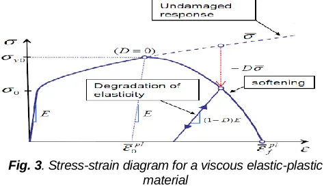
Deletion of the processed material is an integral part of the cutting process. The nature of the deletion of the processed material largely determines the cutting forces, the type of chips obtained, the accuracy of processing, etc. The fracture criterion for viscous materials is usually formulated either as a limiting value of plastic strain or as a limiting value of the energy of plastic strain (the area under the stress – strain curve (Fig. 3)).
Fig. 3. Stress-strain diagram for a viscous elastic-plastic material
The diagram (Fig. 3) shows the behavior of a viscous elastic-plastic material under tension up to complete failure. At stresses from 0 to σ0, the material is strained elastically; in the stress interval from σ0 to σy0, the material is hardened. Failure begins at the σy0 point. When passing through this point, the voltage is described by the formula:
σ = (1-D)
(16 )
D — is a value ranging from 0 to 1, which displays the degree of damage accumulation. At D = 1, the material is deleted, and the element is removed from the grid,
is the stress that would have occurred at this point in the absence of fracture, as a result of further hardening. For brittle materials, the elongation at break is very small, while the value of σв can be significant. Therefore, when choosing the value of plastic strain as the criterion for the fracture of brittle material, a significant error will occur, while the application of the criterion in stresses will provide an exact solution to the problem. For brittle materials, the condition can be selected as a criterion for failure:σ σв
(17 )
The fracture process can be implemented in various ways, but the most common is the modeling of fracture by removing elements, provided that the criterion of fracture is met. In those FEs where the fracture criteria are met, the Cauchy stress tensor is set equal to zero, and these elements are removed from the grid. The physical fracture criterion does not always provide numerical stability of the calculation. Restructuring of the FE grid through a given time step is used to increase the numerical stability. The process of friction between the front surface of the tool to be processed and the chips and the back surface of the tool and the workpiece is the most complex and poorly studied physical process, which manifests itself in the processing of metals by cutting. To describe the friction process between the tool, chips and the workpiece, different models are currently used [20], [21], [23], [24]. The most widely used is the Coulomb friction model:
τ σ
(18 )
where τ — contact shear stress, σ — normal contact stress, μ — Coulomb friction coefficient. This approach becomes possible if we use the concept of the average coefficient of friction μs on the contact surface of the chip and tool, which generally characterizes the processes that occur in this area. The simplicity of the mathematical dependence, the visibility of this indicator and the results of forecasting integral indicators (for example, cutting forces) that are sufficiently consistent with the experiment have provided widespread use of the average coefficient of friction, both in analytical and finite element models of the cutting process.
6 THE
DISCUSSION
OF
THE
RESULTS
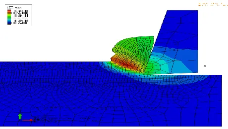
In the present work we obtained the ratios that describe the basic physical processes that occur during the metal processing by cutting. The study showed that simplified models of physical processes give the greatest accuracy. So, the most correct description of the friction process between the cutter and the chips is the Coulomb friction model, and the behavior of the processed material with large deformations and fractures is most accurately described using the Johnson-Cook model, which applies empirical coefficients. Based on the obtained ratios, a finite element model of the rectangular cutting process was formed, in which plastic strains, friction, and also temperature effects were considered. Fig. 4 shows the temperature distribution in the cutting area.
Fig. 4. Temperature distribution in the cutting area
7 CONCLUSION
The obtained ratios describe almost the entire complex of physical phenomena occurring during metal cutting. The described models are built under the assumption of processing with an absolutely rigid tool without vibrations. An introduction to the model of tool vibrations would allow us to study the nature of the occurrence of vibrations during metal cutting. This is possible with modern FE applications such as Abaqus and Ansys. Cutting process modeling using the above ratios showed a good correlation with the results of experimental studies conducted by other authors. In terms of assessing cutting forces and temperatures in the cutting area, the error didn’t exceed 15 percent.
REFERENCES
[1] L. Segerlind, Application of the finite element method.
Moscow: Mir, 1979,
http://pnu.edu.ru/media/filer_public/2013/04/10/6-13_segerlind_1979.pdf
[2] P. Yascheritsyn, Theory of cutting. Minsk: Novoe Znanie, 2005, ISBN 985-475-195-3.
[3] F. Ducobu et al., ―Experimental contribution to the study of the Ti6Al4V chip formation in orthogonal cutting on a milling machine,‖ International Journal of Material Forming, vol. 8, no. 3, pp. 455-468, 2015, https://doi.org/10.1007/s12289-014-1189-4
[4] Yu. Vinogradov, ―Cutting process modeling by the finite element method‖, dissertation. Tula state University, Tula, Russia, 2004, https://lib-bkm.ru/13739
[5] D. Kryvoruchko, Basics of 3D modeling of processes of machining by finite element method: tutorial. Sumy: SSU publishing house, 2009, ISBN 978-966-657-273-1
[6] V. Kalhori, ―Modelling and simulation of mechanical cutting,‖ PhD dissertation, Luleå tekniska universitet,
2001,
http://www.diva-portal.org/smash/record.jsf?pid=diva2%3A998954&dswid =-2130
[7] M. Bashistakumar and B. Pushkal, ―Finite element analysis of orthogonal cutting forces in machining AISI 1020 steel by using a carbide tip tool,‖ Journal of Engineering Sciences, vol. 5, no. 2, pp. A1-A10, 2018, doi: 10.21272/jes.2018.5(2).a1
[8] W. Niu et al., Modeling of orthogonal cutting process of A2024-T351 with an improved SPH method. The International Journal of Advanced Manufacturing Technology, vol. 95, no. 1-4, pp. 905-919, 2018, https://doi.org/10.1007/s00170-017-1253-6
[9] B. Takabi and B.L. Tai, ―Finite Element Modeling of Orthogonal Machining of Brittle Materials Using an Embedded Cohesive Element Mesh,‖ Journal of Manufacturing and Materials Processing, vol. 3, no. 2(36), pp. 1-14, 2019, https://doi.org/10.3390/jmmp3020036 [10]T. Belytschko et al., Nonlinear Finite Element for Continua
and Structures, New York, USA: John Wiley & Sons Ltd, 2000, https://www.twirpx.com/file/1528311/
[11]F. Ducobu et al., ―Finite element modelling of 3D orthogonal cutting experimental tests with the Coupled Eulerian-Lagrangian (CEL) formulation,‖Finite Elements in Analysis and Design, no. 134, pp. 27-40, 2017,
https://doi.org/10.1016/j.finel.2017.05.010
[12]M. Watremez et al., ―Finite element modelling of orthogonal cutting: sensitivity analysis of material and contact parameters,‖ International Journal of Simulation and Process Modelling, vol. 7, no. 4, pp. 262-274, 2012,
https://doi.org/10.1504/IJSPM.2012.049820
[13]P.L.B. Oxley, ―Mechanics of machining: an analytical approach to assessing machinability,‖ Journal of Applied Mechanics, vol. 57, no. 1, pp. 253, 1990, https://doi.org/10.1115/1.2888318
[14]A Vereshchaka and V. Kushner, Cutting of metals: tutorial, Moscow: Vysshaya shkola, 2009, ISBN 978-5-06-004415-7
[15]F. Ducobu et al., ―On the importance of the choice of the parameters of the Johnson-Cook constitutive model and their influence on the results of a Ti6Al4V orthogonal cutting model.‖ International Journal of Mechanical Sciences, 122, pp. 143-155, 2017, https://doi.org/10.1016/j.ijmecsci.2017.01.004
[16]J. Shi, and C.R. Liu, ―The influence of material models on finite element simulation of machining,‖ Journal of Manufacturing Science and Engineering, vol. 126, no. 4, pp. 849-857, 2004, https://doi.org/10.1115/1.1813473 [17]A. Shrot and M. Bäker, ―Determination of Johnson–Cook
parameters from machining simulations,‖ Computational Materials Science, vol. 52, no. 1, pp. 298-304, 2012,
https://doi.org/10.1016/j.commatsci.2011.07.035
[18]G.R. Johnson, ―A constitutive model and data for materials subjected to large strains, high strain rates, and high temperatures,‖ Proc. 7th
Inf. Sympo. Ballistics, pp. 541-547, 1983, https://edoc.pub/a-constitutive-model-and- data-for-metals-subjected-to-large-strains-high-strain- rates-and-high-temperatures-g-johnson-w-cookpdf-pdf-free.html
[19]R. Kesharwani, ―High temperature behavior of copper,‖ Master thesis, National Institute of Technology
Rourkela-769008, Orissa, India, 2010,
http://ethesis.nitrkl.ac.in/2054/
[20]T. Özel and E. Zeren, ―Finite element modeling of stresses induced by high speed machining with round edge cutting tools,‖ Proceedings of IMECE, vol. 5, pp. 1-9, 2005,
https://pdfs.semanticscholar.org/d0ea/c8b2c741467c1856 efbd9220cd8c6d09066c.pdf
[21]T. Özel and T. Altan, ―Determination of workpiece flow stress and friction at the chip–tool contact for high-speed cutting.‖ International Journal of Machine Tools and Manufacture, vol. 40, no. 1, 133-152, 2000, https://doi.org/10.1016/S0890-6955(99)00051-6
1980 Effects of damage criteria and particle density.‖ Journal of
Manufacturing Processes, no. 30, pp. 523-531, 2017, https://doi.org/10.1016/j.jmapro.2017.10.020
[23]A. Malakizadi et al., ―Influence of friction models on FE simulation results of orthogonal cutting process,‖ The International Journal of Advanced Manufacturing Technology, vol. 88, no. 9-12, pp. 3217-3232, 2017, https://doi.org/10.1007/s00170-016-9023-4