EFFECT OF GOVERNMENT EXPENDITURE ON ECONOMIC GROWTH IN RWANDA (2005-2015)

(1)

Licensed under Creative Common Page 108

http://ijecm.co.uk/

ISSN 2348 0386

EFFECT OF GOVERNMENT EXPENDITURE ON

ECONOMIC GROWTH IN RWANDA (2005-2015)

Amos Ochieng

Jomo Kenyatta University of Agriculture and Technology, Kigali, Rwanda

amosochieng88@gmail.com

Jaya Shukla

Lecturer, Jomo Kenyatta University of Agriculture and Technology, Kigali, Rwanda

js.jayashukla@gmail.com

John Paul Okello

Lecturer, KIM University, Kigali, Rwanda

okellojohn85@yahoo.com

Joseph Oduor

Director, Kampala University College, JUBA, South Sudan

joekoduor@yahoo.com

Abstract

(2)

causality. The impulse response and VDA results revealed that expenditure on agriculture, education and health had positive effects on GDP, sports and culture expenditure had mixed reactions and Physical infrastructure expenditure had negative effects. The study recommended that agriculture and social sector expenditures to be increased while infrastructure expenditure be streamlined.

Keywords: Minecofin, Government Expenditure, Expenditure Growth, Economic Growth, Stationarity, Granger causality, Vector Auto Regression (VAR)

INTRODUCTION

After the genocide of 1994 which brought the Rwandan economy to grassroots, the government

embarked on reviving the economy through adopting measures that stimulates economic

growth in various sectors of the economy. This called for expansion of government expenditure

in various sectors of the economy in order to achieve a steady economic growth. Over the years

government expenditure has grew more rapidly than the growth rate of GDP. This raises

concern among policy makers and requires an investigation as to why GDP is growing at a

slower rate despite the government effort to expand its expenditure in order to stimulate rapid

economic growth. Given this fiscal scenario, there is need to study the impact of government

expenditure on economic growth in order to explain the wide range difference between

government expenditure growth rate and GDP growth rate.

The relationship between Government expenditure and economic growth is a key area

of study. The question is whether government expenditure increases the long run steady growth

rate. Generally, government expenditure on physical infrastructure and human capital speeds

up growth though the sources of such finances can slow down growth (Landau, 1983;

Devarajan, 1993; Cashin, 1995; Kneller, 1999).This is due to the negative impact of taxes for

example on investment. High taxes discourage investments and this slows down economic

growth (Musgrave and Musgrave, 1989).Government expenditure can increase output directly

or indirectly through different ways as examined by Lin (1994).These ways include provision of

public goods, social services like health and education and through promotion of exports by

offering subsidies.

Government expenditure can impact positively or negatively depending on its form.

According to Barro (1990), expenditure on investment and productive activities including

(3)

government consumption expenditure e.g. wages and salaries and public debt servicing is

expected to be growth-retarding.

Government expenditure can contribute to economic growth directly or indirectly (Barro

& Sala-i-Martin, 1992).According to Barro, direct effect is where government expenditure results

to increase in physical and human capital stock reflecting higher flows of government funds, for

example expenditure on education, health and physical infrastructure. An indirect effect can be

seen on its impact on marginal productivity of production factors. For example expenditure on

research and development improves the productivity of capital, labor. Similarly expenditure on

security lowers production cost of firms inform of security expenses for the employees and

assets.

There is growing evidence that suggest that in developing countries, externalities

associated with infrastructure expenditure may be important in enhancing growth (Landau,

1985). Indeed, it has been found that infrastructure may have an impact on human capital as

well. According to(Meltzer, 1992) (2007), government expenditure on infrastructure affects

growth not only through its direct impact on investment and the productivity of factors in the

private sector, but also through health and education outcomes. Government expenditure that

facilitates access to clean water and sanitation helps to improve health and thereby labor

productivity. These expenditures can be in the form of provision of electricity, which is essential

for the functioning of hospitals and the delivery of health services, and better transportation

networks, which contribute to easier access to health care, particularly in rural areas. In

addition, there is evidence of direct linkages between infrastructure and education. Education

allows for more training and greater access to learning technologies. Enrollment rates and the

quality of education tend to improve with better transportation networks, particularly in rural

areas. Greater access to sanitation and clean water in schools tend to raise attendance rates.

According to Kosimbei (2013) and Maingi (2010), there are two major traditional

approaches that analyses the effect of government expenditure on economic growth. They

include the Keynesian approach and the monetarist approach. Keynesians believe that the key

to both a healthy economy and correcting recessions and depressions is doing whatever it takes

to entice consumers to continue spending. According to Keynes, during recession, households

save more than they consume. This is due to the fear of loss of job in the near future. This trend

worsens the economy more since reduced consumption makes businesses to close down and

hence investment falls. To break the cycle, Keynesian economists think that the government

should increase its spending to compensate for the slowdown in aggregate demand.

Government spending would help to boost productivity and therefore protect jobs, which in turn

(4)

According to Monetarist approach led by Friedman, sustained money growth in excess of the

growth of output produces inflation (Branson, 1989).To reduce inflation, the growth in the money

supply needs to be controlled and thus the need to control or reduce government expenditure

(Brunner and Meltzer, 1992). This theory further argues that tax financed government

expenditure crowds out private investment (Ahmed, 1999). This is because when government

expenditure is tax-financed, any extra expenditure calls for more taxation. A higher tax burden

reduces the disposable income for individuals, which results to a reduction in consumption,

lower savings and hence lower investment. On the other hand, higher tax burden on

corporations and businesses result to decreased profits and thus reduces expansion and

development aspects. If the government decides to borrow from money or capital market to

finance its expenditure, it has a future obligation to repay the loan and its interest, which places

a burden on the future generation. These factors result to crowding out of private investment in

the course of funding government expenditure (Ahmed, 1999).

The modern approach states that labor force must be provided with more resources i.e.

physical capital, human capital and technology for increased productivity to be achieved. This

implies that the only way a government can affect economic growth, at least in the long-run, is

via its impact on investment in capital, education and research and development. The approach

makes improved education the key to achieving economic growth.

Trend in government expenditure and economic growth in Rwanda

The trend in government expenditure and economic growth in Rwanda is shown in the figure 1.

Figure 1: Trends in government expenditure and GDP growth

Source: GDP and Public expenditure reports, NISR, 2016 and Minecofin 0

10 20 30 40 50 60

2004 2006 2008 2010 2012 2014 2016

PE

R

CE

N

TA

GE

YEAR

GDPGR(%)

(5)

From figure 1 above initially there was a sharp increase in government expenditure from 2005 to

2007.This was accompanied by a fall in the GDP growth rate. In 2007/2008 financial year

government expenditure growth rate declined and then rose up in the following financial year,

2008/2009.This period saw a rise and a fall in GDP growth rate within the two years.

Followed was a downward trend in expenditure growth rate for the next 3years which

was accompanied by an increasing trend in GDP growth rate. There was a rapid increase and a

fall in government expenditure growth rate from 2011 to 2013 accompanied by a slight increase

and a fall in GDP growth rate. The last financial year was accompanied by a fall in government

expenditure growth rate and a rise in GDP.

Generally the expenditure growth rate is greater than the GDP growth rate evidenced by

the gap in the figure 1 above. There was a fluctuation in government expenditure growth rate

during the period of study though there was an increasing expansion of government expenditure

every year. The GDP growth rate is generally accompanied by a steady decline, a minimal rise

and fall, steady increase overtime and then a minimal rise and fall. Expenditure growth rate was

highest in 2011/2012 which was accompanied by a rise in GDP growth in line with the

Keynesian theory that there a positive relationship between government expenditure and

economic growth. The GDP growth rate was highest in 2008 though there was a decline in

expenditure growth in the same year.

Trend in composition of government expenditure in selected sectors in Rwanda

In order to explain the growth in the overall government expenditure, we consider its breakdown

into different categories. Government expenditure can be broadly classified in terms of purpose

as development expenditure and recurrent expenditure. Capital expenditure refers to the

amount spent in the acquisition of fixed (productive) assets (whose useful life extends beyond

the accounting or fiscal year), as well as expenditure incurred in the upgrade/improvement of

existing fixed assets such as lands , building, roads, machines and equipment, etc., including

intangible assets. Expenditure in research also falls within this component of government

expenditure. Capital expenditure is usually seen as expenditure creating future benefits, as

there could be some lags between when it is incurred and when it takes effect on the economy.

They are more discretionary and are made of new programs that are yet to reach their stage of

completion (Ag’enor, 2007).

Recurrent expenditure refers to expenditure of recurrent expenses that are less

discretionary and are made on ongoing programs or activities. It constitutes of wages and

salaries, administration, transfers payment, debt repayment and welfare services. Recurrent

(6)

work, save and invest (Ag’enor, 2007). Various ministries in Rwanda incur expenditures from

government budget allocations which vary from one ministry to another every financial year

(figure 2). This study will concentrate on 5 sectors namely, agriculture, sports and culture,

health, education and infrastructure.

Figure 2: Distribution of public spending in selected sectors in Rwanda

Source: public expenditure data reports from Minecofin

From the figure 2 above, the Rwandan government invested greater percentage of the budget

on education and infrastructure sectors. Expenditure on education rose initially, decreased from

2007 and then started to rise again from 2009 reaching maximum in 2011 before exhibiting a

downward trend for the remaining period. Infrastructure expenditure increased upto 2008 and

started to fall before rising again after 2009 reaching a maximum in 2013 before dropping.

Health expenditure remained fairly constant up to 2007, dropped and then started to rise again

after 2008 until 2010 beyond which it exhibited a rise and fall every year for the rest of the

period. Agriculture expenditure had an increasing trend up to 2010 after which showed a steady

trend for the rest of the period. Sports and culture had a fairly constant trend with expenditure

taking less than 2%of the total budget execution within the study period.

Statement of the problem

The causes of much of the variations in economic growth rate and expenditure growth rate in

Rwanda are not well understood. Particularly, the effect of government expenditure on

economic growth has not been explored well. Several studies have been carried out on

government expenditure and economic growth in several countries and they give different 0 5 10 15 20 25 30

2004 2006 2008 2010 2012 2014 2016

b u d ge t al lo cation to sec to

rs as a

(7)

findings. (Landau, 1983; Diamond, 1984; Barro, 1990; Davarajanet al. 1993; Kweka, 1995;

Colombier, 2000; Maingi, (2008),Njuguna, (2009).From these studies, the effect of government

expenditure on economic growth appear unconvincing. Despite this uncertainty, theory tells us

that government expenditure has a positive effect on economic growth (Keynes, 1936;

Solow-Swan, 1956; Musgrave and Musgrave, 1989; Barro, 1990; Barro and Salai-i-Martin, 1992, and

1995).

In Rwanda, government expenditure has been rising rapidly for the last ten years as a

move by the government to stimulate economic growth. The impact of these increases in

government expenditure on economic growth appears to be minimal as shown by a steady but

slow economic growth rate. The government of Rwanda spends substantial amounts of money

annually on physical infrastructure, agriculture and social sectors such as education, health

care, sports and culture, public order and national security, defense and general administration

as evidenced by budget execution. From theory, when there is an increase in government

expenditure in these sectors, it is expected that the economy will exhibit a rapid positive

economic growth rate, but this does not seem to happen in Rwanda. This could be due to

non-growth-enhancing expenditures that crowd-out outlays that are meant to boost economic growth

(Colomber, 2000). Therefore, the issue of which government expenditure can foster permanent

movements in economic growth in Rwanda becomes important and needs to be investigated.

General objective of the study

The general objective of this study was to analyze the effect of government expenditure on

economic growth in Rwanda for the period between 2005 and 2015.

Specific objectives of the study

i. To examine the effect of physical infrastructure expenditure on economic growth

ii. To determine the effect of agriculture expenditure on economic growth

iii. To establish the effect of social sector expenditure on economic growth

Research hypotheses

A hypothesis is an explanation for certain behavior, patterns, phenomenon or events that have

occurred or will occur (Gay, 1996).The research was guided by the following working

hypotheses:

i. Physical infrastructure has a significant effect on economic growth.

ii. Agriculture has a significant effect on economic growth.

(8)

Licensed under Creative Common Page 115 Justification of the study

The study from the onset was important since it enabled completion of my Master’s degree

program in economics of JKUAT. Since 2005, Rwanda has gone through substantial structural

changes in various sectors of the economy. The study attempted to provide an empirical

analysis of the impact of government expenditure components on economic growth. This was

important to policy makers since they were able to identify the main drivers of expenditure

growth and be able to identify which component of government expenditure to be targeted for

any fiscal action in line with both short run and long run growth objectives of the country.

Furthermore the study analyzed both theoretical and empirical literature on government

expenditure and economic growth. This opened the way for further studies.

Scope of the study

The study was limited to the period between 2005 and 2015 since this period there was mass

increase in government spending and the data was readily available. Economic growth can be

affected by both fiscal and monetary policies. This study concentrated on fiscal policy effects

particularly government expenditure leaving out government revenue as another form of fiscal

policy. Government expenditure was categorized in terms of actual budget execution to various

ministries. The study was limited to the following sectors, physical infrastructure, agriculture and

social sectors specifically education, health and sports and culture.

LITERATURE REVIEW

Theoretical review Wagner’s theory

This theory was put forward by German political economist, AdolphWagner (1835-1917). He

argued that government growth is a function of increased industrialization and economic

development. Wagner stated that during the industrialization process, as the real income per

capita of a nation increases, the share of public expenditures in total expenditures increases.

The law cited that "The advent of modern industrial society will result in increasing political

pressure for social progress and increased allowance for social consideration by industry."

Wagner (1893) designed three focal bases for the increased in state expenditure. Firstly,

during industrialization process, public sector activity will replace private sector activity. State

functions like administrative and protective functions will increase. Secondly, governments

needed to provide cultural and welfare services like education, public health, old age pension or

retirement insurance, food subsidy, natural disaster aid, environmental protection programs and

(9)

and large firms that tend to monopolize. Governments will have to offset these effects by

providing social and merit goods through budgetary means.

In his Finanzwissenschaft (1883) and Grundlegung der politischen Wissenschaft (1893),

Adolf Wagner pointed out that public spending is an endogenous factor, which is determined by

the growth of national income. Hence, it is national income that causes public expenditure. This

theory is relevant in Rwanda since the increased GDP of Rwanda overtime accelerated by

industrialization has attracted more government expenditure in order to expand provision of

public goods and other essential state services. Some of the flaws of this theory is that it

concentrated on the demand side of the government expenditure while overlooking the supply

side and it also dwelt on industrialization as the only driving force for increased public spending.

Peacock and Wiseman’s political constraint model

Peacock and Wiseman (1890-1935) in their analysis of time path pattern of government

expenditure established the displacement effect.it is based on political theory of government

expenditure determination that government likes to spend more money and citizens do not like

to pay taxes. The model assumes that there is some tolerable level of taxation that act as a

constraint on government behavior. As the economy grows, tax revenue would rise and hence a

rise in government spending in line with GNP (Peacock & Wiseman 1961).

During period of social upheaval such as war, famine or some large-scale social

disaster, the gradual upward trend in government expenditure would be distorted (displaced

upward). In order to finance the increase in government expenditure, the government may be

forced to raise taxation level, a policy which would be regarded as acceptable to the electorate

during period of crises. This is called the displacement effect (Peacock & Wiseman, 1961).

There will be a new level of "tax tolerance". Individuals will now accept new taxation levels,

previously thought to be intolerable. Furthermore, the public expect the state to heal up the

economy and adjust to the new social ideas, or otherwise, there will be the inspection effect.

The net result of these two effects is occasional short- term jumps in government expenditure

within a rising long-term trend (Peacock and Wiseman, 1961).

This theory is relevant in Rwanda since after the genocide of 1994, there was a rapid

rise in government expenditure to heal the country from the effects of war. The theory has some

weaknesses such as; it explains the economic upheaval as the cause of increased government

expenditure yet in Rwanda public expenditure has been rising overtime yet there is peace, its

long since war of 1994 and yet the public spending keeps on rising; the theory also considers

(10)

as domestic and foreign borrowing, foreign aid and income from sale of goods and services

(Brown et al, 1996).

Keynesian theory

This theory was put forward by economist; John Maynard Keynes (1883-1946).He argued that

government intervention was necessary in the short run to save the economy from depression.

He argued that in the long run we are all dead. Increasing saving during depression will not help

but instead spending saves the economy. Increased spending raises the purchasing power of

people and hence consumption increases. Producers expand their production and hence

employment is created. He further said that expansion of government expenditure should be

done with a lot of care since too much of it could lead to inflation.

The flaws of Keynes theory are: The theory tended to give rise to the phenomenon

known as stop-go. That is, in periods of high unemployment, the government would expand

aggregate demand. This would reduce the unemployment but at the same time tend to create

inflationary pressure so that eventually the government would have to reduce aggregate

demand again. Thus, all go period tended to be followed by stop period and it became difficult to

achieve long term economic growth. A second limitation of the Keynesian model is that it fails to

take adequately into account the problem of inflation. Third, it tends to understate the influence

of money on the real variables in the economy. A change in the money supply, only affects

national income through its effects on the rate of interest.

Monetarist theory

This theory stresses the primary importance of money supply in determining nominal GDP and

the price level (Ahmed, 1999). Friedman (1956) argued convincingly that the high rates of

inflation were due to rapid increases in the money supply. The key to good policy was therefore

to control the supply of money. The foundations of the model were: There is a close relationship

between the changes in the money supply and changes in national income in the long-run,

without government interference the economy will tend towards its „natural‟ rate of

unemployment, velocity of circulation of money is predictable, money changes will only affect

real national income indirectly and the economy is in equilibrium at full employment Monetarists

disliked big government and tended to trust free markets. They did not like government

expenditure and believed that fiscal policy was not helpful in bringing about economic growth.

Where it could be beneficial, monetary policy could do better. Excessive government

expenditure only interferes in the workings of free markets and could lead to bloated

(11)

comings of the model include the following. First, the monetary theory does not offer a complete

explanation of the complex phenomenon of changes in the making of which the non-monetary

factors also significantly matter.

Rostow’s Theory

This theory takes government expenditure as a prerequisite of economic development, its level

being directly related to the stage of development that a country has reached. In the early stage

of economic growth and development, public investment as a proportion of the total investment

of the economy is found to be high. The public sector provides social infrastructure overheads

such as roads, transport infrastructure, sanitation services, law and order, health, education and

other investments in human capital, which are all necessary to gear up the economy for takeoff

into the middle stages of economic and social development (Musgrave and Musgrave, 1989). In

the middle stages of growth, the government continues to supply investment goods, but this

time public investment is complementary to the growth in private investment. During the two

stages of development, markets failures exist, which can frustrate the push towards maturity,

hence increase in government involvement in order to deal with these market failures. In the

mass consumption stage, income maintenance programs and policies designed to redistribute

welfare grows significantly relative to other items of government expenditure, and also relative

to GNP (Musgrave and Musgrave, 1989).

Empirical review

Harerimana (2016) conducted a study on the analysis of government spending on agriculture

sector and its effect on economic growth in Rwanda using General Method of Moments and

OLS. The results indicated that there is a long run relationship between agriculture expenditure

and economic growth and that there is a positive significant effect of agriculture sector on

economic growth in Rwanda.

Edward (2012) examined the interrelationships between public spending composition

and Uganda’s development goals including economic growth and poverty reduction using

dynamic computable general equilibrium model. The results demonstrated that public spending

composition on productive sectors such as agriculture, energy, water, health and

complementary infrastructure such as roads has positive impact on economic growth and

poverty reduction while unproductive sectors such as public administration and security had a

negative impact on economic growth and poverty reduction.

Albala and Mamatzakis (2001) using time series data covering 1960-1995 to estimate a

(12)

and significant correlation between public infrastructure and economic growth. The study

reported that public investment crowds out private investment. One major weakness of the

study was that it omitted impact of important variables such as education, health care and public

order and security.

Fasoranti (2012) while conducting a study on the effect of government expenditure on

infrastructure on the growth of Nigerian economy found out that expenditure on healthservices,

transport and communication imparted negatively on growth. Moreover, expenditure on

agriculture and security had no impact on the growth of the economy while expenditure on

education, environment and housing and on water resources had a positive impact on economic

growth.

Olopade and Olapade (2010) assess how fiscal and monetary policies influence

economic growth and development. The essence of their study was to determine the

components of government expenditure that enhance growth and development, identify those

that do not and recommend those that should be cut or reduced to the barest minimum. The

study employs an analytic framework based on economic models, statistical methods

encompassing trends analysis and simple regression. They found no significant relationship

between most of the components of expenditure and economic growth.

Maingi (2010), while studying the impact of government expenditure on economic growth

in Kenya found out that in the long run expenditure on economic affairs, defense, education,

government investment, general administration and services and physical infrastructure have

positive impacts on economic growth. In the short run health care, public order and national

security have positive impact on economic growth, whereas, public debt servicing had negative

impact on economic growth.

Kosimbei (2013) while conducting research on the impact of government expenditure

components on economic growth in Kenya found out that public expenditure component like

education, transport and communication and public order and security are the major drivers of

economic growth. The study found out that Public expenditure on health impacted negatively on

economic growth.

Naftally (2014)while conducting research on the effect of government expenditure on

economic growth in East Africa using the disaggregated model found out that expenditure on

health, defense, agriculture and openness were positively related to economic growth while

expenditure on education, terms of trade and population growth had a negative impact on

economic growth. However the study concentrated majorly on 3 countries namely Kenya,

(13)

Abbas and Abdul (2016) conducted a research on the impact of government expenditure on

agricultural sector and economic growth in Pakistan over the period 1983 to 2011using time

series data. They used null hypothesis that agriculture expenditure does not have impact on

economic growth which they finally rejected. Study found a positive relationship between

agricultural output and economic growth. An increase in agricultural output leads to a positive

economic growth. They recommended that the government should increase expenditure on

agriculture sector.

Mustapha (2015), while analyzing empirically the impact of education expenditure on

economic growth in Nigeria using granger causality analysis found out that there is no causality

between Real Growth Rate of gross domestic product and Total government expenditure on

education but there is bi-directional causality between Recurrent Expenditure on Education and

Total government expenditure on education. He further found out that while Primary School

Enrolment does not Granger cause Total government expenditure on education, the latter does

Granger cause the former. No causality between Recurrent Expenditure on Education and Real

Growth Rate of gross domestic product and also no causality between Primary school

enrolment and Real Growth Rate of gross domestic product.

Mekdad et.al (2014) examined the effect of public spending on economic growth in

Algeria for the period 1974-2012. Their study used Ordinary Least Square and Johansen

Co-integration test and causality tests, their results showed that public spending on education

affects economic growth positively.

Figure 3: Conceptual framework

Physical infrastructure sector expenditure

 Budget allocation to physical infrastructure

Agriculture sector expenditure

 Budget allocation to agriculture

Social sector expenditure

 Budget allocation to education sector

 Budget allocation to health sector

 Budget allocation to sports and culture sector

Economic growth

 GDP Growth Rate

(14)

Licensed under Creative Common Page 121 Critical review of literature

The question of whether or not public expenditure stimulates economic growth has dominated

theoretical and empirical debate for a long time. One viewpoint believes that government

involvement in economic activity is growth enhancing, but an opposing view holds that

government operations are inherently inefficient, bureaucratic and therefore stifles rather than

promotes growth, while some studies still are of the view that public expenditure is

indeterminate of economic growth (Najkamp & Poot, 2002). In the empirical literature, results

are equally mixed. It is evident that most of the empirical literatures focuses on developed

countries, even so all of them have not come up with similar relationship between public

expenditure and economic growth, and some sharply contradict others (Jerono, 2002).

The methodologies used in those literatures reviewed might not be very applicable in

Rwanda due to divergence in geographical region, political difference and level of economic

growth between the studied countries and Rwanda. In Rwanda studies on public expenditure

impact on economic growth have not been carried out. Studies that have been carried out in the

neighboring developing countries like Kenya and Nigeria and the East Africa as a

disaggregated model have reported divergent results as to the impact of public expenditure on

economic growth (Jerono, 2002). Finally with a lot of contention, the underlying argument is that

public expenditure is capable of enhancing economic growth in short and in the long run in both

developing and developed countries.

Summary of the literature

From the review of the studies, the effect of public spending on economic growth is fundamental

in any economy. There are divergent results on these studies depending on the variables of

public spending used, the methodology and the location. Public spending is fundamental for a

countries growth and therefore there is need to inquire more about the effect of such public

expenditures on economic growth. Moreover with the increasing and ever changing world i.e.

from less developed to developing nations and increasing need for industrialization ,there is

need for changes in the allocation of public funds to various sectors to achieve economic

growth. In summary public spending is one of the fiscal policy tools of achieving economic

growth and requires deeper investigation.

Research gap

Most of the literature on government expenditure and economic growth gives different results on

the relationship and effects of government expenditure and economic growth depending on the

(15)

of the studies were carried out on developed countries and less on developing countries as

evidenced from the theoretical literature. The few studies done in developing countries did not

look at Rwanda in isolation. This study therefore sought to add knowledge about government

expenditure and economic growth on developing countries by looking at Rwanda. This is a gap

that existed and needed to be filled. The relationship between government expenditure and

economic growth has been giving different results from the previous literature depending on

how the government expenditure is categorized. Studies by Devaragan (1993) grouped

government expenditure into productive and non-productive categories while Stephen Gitahi

(2014) categorized government expenditure in terms of development and recurrent expenditure.

Only Maingi (2010) looked at government expenditure in terms of annual budget allocation to

various Ministries as a percentage of GDP. He found out that expenditure on education, health,

defense, economic affairs and infrastructure had a positive impact on economic growth while

public debt servicing had a negative impact on economic growth.

METHODOLOGY

Research Design

A research design is the overall strategy of integrating the various components of the study in

coherent and logical manner in order to effectively address the research problem. (Labaree,

2009). The study utilized quantitative research design because it involves systematic empirical

investigation of observable phenomena via statistical or numerical data. This study aims at

establishing the impact of public expenditure components on economic growth in Rwanda.

Measurement of various variables of public expenditure and economic growth is crucial in this

research since it shows connection between empirical observation and mathematical

expression of quantitative relationships.

There are basically three dimensions of quantitative research design, descriptive

research which seeks to describe the current status of a variable or a phenomenon,

correlational design which explores the relationship between variables using statistical analysis

and experimental design which involve use of scientific method to establish a cause-effect

relationship. Since the study seeks to investigate the impact of government expenditure on

economic growth, descriptive and correlational quantitative research design is justified.

Descriptive studies are aimed at finding out “what is,” so observational and survey methods are

frequently used to collect descriptive data (Borg & Gall, 1989). Descriptive research is unique in

the number of variables employed. Like other types of research, descriptive research can

include multiple variables for analysis, yet unlike other methods, it requires only one variable

(16)

correlations between multiple variables by using tests such as Pearson's Product Moment

correlation, regression, or multiple regression analysis which suited this research because the

study used multi-variate time series data. The study employed an econometric model to study

the relationship between the variables under study. VAR model was employed to assess the

effects of government expenditure components on economic growth. Similar method was used

by other researchers like Albala (2001) in Chile, Fasoranti (2012) in Nigeria, Maingi (2010) in

Kenya, (Sharabati et al., 2010) in Jordan.

Data collection and procedure

The study used time series secondary data. This was enhanced by easy accessibility of

secondary data from government’s data base and also to be consistent with the previous

researchers who also used secondary data such as Fasoranti (2012) and Kosimbei (2013)

Government expenditure was classified in terms of budget execution in selected sectors in

Rwanda. These are agriculture, health, sports and culture, education and physical

infrastructure. Quarterly data on these variables was obtained from Ministry of Finance and

Economic Planning (Minecofin) for the period 2005 to 2015. Economic growth was in terms of

GDP output within the study period. The data was obtained from National Institute of Statistics

of Rwanda annual report data base.

Several previous researches on government expenditure and economic growth utilized

time series secondary data though the time frame and geographical location was different from

one research to another as shown in the empirical review. This study is therefore consistent with

the previous researches.

Data Analysis Approach

The study addresses three objectives. The analysis of effects requires testing for the

relationships first between the variables under study. This was achieved by carrying out

multivariate cointegration test and granger causality test. To analyze the effects of government

expenditure components on economic growth, the researcher utilized vector autoregresion

model and subsequently the impulse response analysis and variance decomposition analysis.

Definition and measurement of variables

Economic Growth (GDP)

This is the percentage rate of increase in gross domestic product. It captures the change in

value of goods and services produced in a given economy for a specified period of time. It was

(17)

Licensed under Creative Common Page 124 Education expenditure

This is the share of expenditure in education to total government expenditure. It includes the

expenditure the government incurs to fund basic up to higher education, by paying teachers and

lecturers, construction of learning infrastructure such as classrooms, lecture halls, offices and

purchase of learning equipment. It also includes expenses on scholarships whether local or

abroad. (Fasoranti, 2012)

Health expenditure

This is the share of public expenditure on health to total government expenditure. It includes the

amount the government spends in construction of hospitals building structures, equipping the

hospital institution with equipment and drugs, training of doctors and nurses and paying their

salaries. (Maingi & Kosimbei, 2013)

Infrastructure expenditure

This is the share of public funds over the total government expenditure directed to activities

such as, construction of air and seaports, construction of highways, fiber optic cable connection

lay outs. (Buhari, 2000)

Agriculture expenditure

This is the share of public funds over the total government expenditure that is spent on activities

such as providing fertilizer for farmers, research and extension services, veterinary services,

educational workshops, paying salaries for employees etc. (Gideon and Njenga, 2013)

Sports and culture expenditure

This is the share of public expenditure over the total expenditure that is spent on activities such

as maintaining tourism sites, cultural functions such as genocide memorial, sports matches,

salaries for employees in the sports and culture ministry etc. (Kosimbei, 2013)

Model Specification

The study was based on Keynesian theory. Keynesian theory states that public expenditure

determines economic growth. During recession a policy of budgetary expansion should be

undertaken to increase the aggregate demand in the economy thus boosting the Gross

Domestic Product (GDP), the employment rises, income and profits of the firms increase, and

this would result in the firm’s hiring more workers to produce the goods and services needed by

(18)

Y = f (GE)....(3.1) The Keynesian modeled economic growth as a function of public expenditure.

Y = f (GE)……………..(3.2) Jerono (2009) defined total public expenditure as a function of summation of all individual

government expenditure in all components.

GE = f (government expenditure in all components) ……… (3.3)

In this study combining the two models will yield a richer econometric model that will facilitate

estimation. The government expenditure (GE) is defined as the five components; this modification will help us investigate the impact of government expenditure on economic growth

in Rwanda.

GE= f [(ei, eg,ed,eh, es), Ut]………... (3.4)

And because,

Y= f (GE) according to the Keynesian, Hence

Y = f [(ei, eg, ed, eh, es), Ut]………. ………... (3.5)

Y



0 



1 ei





2 eg





3 ed





4 eh





5 es



ut

……….…….. ………... (3.6) Where;

Y = gross domestic product

ei= infrastructure expenditure

eg = agriculture expenditure

ed= education expenditure

eh= health expenditure

es = sports and culture expenditure

Ut =Error term (causes of economic growth not explained by variables in the model)

Time Series property of the data

In view of the fact that this study will use time series data and inherently it might exhibit some

strong trends, the non-random disposition of the series might undermine the use of some of

econometrics tests such as F and t tests. This is because they can cause rejection of a

hypothesis which would have otherwise not been rejected. This study intends to conduct

stationarity and cointegration tests to mitigate such situations.

In empirical analysis, non-stationarity of time series data is a perennial problem. To

avoid estimating and getting spurious results, the study conducted test for stationarity. To apply

(19)

variables is required ( (Verbeek, 2004), 2004). According to (Brooks, 2008) Brooks (2008), a

stationary series can be defined as one with a constant mean, constant variance and constant

auto-covariance for each given lag. The study used Augmented Dickey Fuller method to test for

stationarity and establish the order of integration. The (ADF) test for stationarity in a series of

say GDP, involves estimating the equations.

Δ𝐺𝐷𝑃=𝛼0+ 𝛽𝑡+𝜃𝑦𝑡−1+ m𝑖=1ρΔGE−i+et (This is for levels)

ΔΔ𝐺𝐷𝑃=𝛼0+ 𝛽𝑡+𝜃Δ𝑦𝑡−1+ m𝑖=1ρΔΔGE−i+et (This is for first differences).There are cases where ADF does not have a drift and a trend but the example has both a drift (intercept) and a trend.

Where 𝛼0 is a drift, m is the number of lags and e is the error term and t is trend. The null hypothesis will be

HO: (𝛼0,) = (𝛼0, 0, 1) (Not stationary) The alternative hypothesis

H1: (𝛼0,) ≠ (𝛼0, 0, 1) (Stationary). If the test reveals that null hypothesis should be rejected then the variable will be said to be stationary.

Testing for Cointegration

The researcher used Johansen Cointegration test method. Cointegration is a technique used to

test for existence of long-term relationship (co-movement) between variables in a non-stationary

series. Before testing for cointegration, it is important to determine the order of integration of the

individual time series. A variable Xt is integrated of order d (1d) if it becomes stationary for the

first time after being differenced d times (Hjalmarsson and Ӧsterholm, 2007). Cointegration also

asserts that 1(1) can be estimated using OLS method and produce non spurious results.

Granger Causality Test

Granger (1969) proposed a time-series data based approach in order to determine causality.

Granger causality shows whether the past values of say X can be able to predict current or

future values of Y. Granger causality test is used to test the causal direction. It is also used to

test for exogeneity and enables the researcher to decide whether to estimate the model using

simultaneous or single equation. Granger causality test has been chosen in this paper for its

favorable response to both large and small samples as evidenced by (Gall, 1989, Salemi, 1982,

Geweke et al., 1983). In this study, it was predicted that the components of government

expenditure affected economic growth. On the same breath the economic growth (GDP levels)

could as well influence the government expenditure and this can lead to our model suffering

from simultaneous bias. Just in case the study estimates the model and gets a statistically

(20)

to conduct the causality test to know the direction of causation. To establish whether it is

government expenditure causing GDP growth or whether it is the GDP leading to growth in

government expenditure or if there is a case of bi-directional causation (a feedback system).

The researcher carried out a pairwise granger causality test of GDP and GE components with

different lags by running the data on E-views software which attracted rejection or acceptance of

null hypothesis. If it is significant then the study conclude that either GDP granger causes GE

(unidirectional), that is a long term relationship between GE and GDP exist whereby the past

values of GDP can be used to predict current or future values of GE. If both granger causes

each other that is GE granger causes GDP and GDP intern granger causes GE then a

conclusion that there is bi-directional relationship is made.

FINDINGS AND DISCUSSION

Unit root test

Quarterly values of all the variables under consideration were used in this study. The period was

from 2005Q1 to 2014Q4.This period was selected because of reliability and availability of data.

In availability of quarterly data that leads to use of disaggregated annual data cause some

estimation and forecasting biases(Gichondo & Kimenyi, 2012).

When time series data is non stationary and used for analysis it may give spurious

results because estimates obtained from such data will possess non constant mean and

variance. Because this study used time series data, it was important to establish the stationarity

of the data or what order they are integrated to make sure that the results obtained are not

spurious. In this regard Augmented Dickey Fuller (ADF) was used to test for unit roots. The unit

roots results of the variable in the model are reported in table 1 and table 2.

Table 1: Stationarity test (at level) results

Variable At level ADF Critical values at probability Agriculture

expenditure

Intercept and trend

-4.117322 1% -4.211868 5% -3.529758 10% -3.196411

0.0127

Infrastructure expenditure

,, -2.068879 1% -4.211868 5% -3.529758 10% -3.196411

0.5464

Education expenditure

,, -3.120828 1% -4.211868 5% -3.529758 10% -3.196411

(21)

Licensed under Creative Common Page 128 Health

expenditure

,, -2.337312 1% -4.211868 5% -3.529758 10% -3.196411

0.4050

Sports and culture expenditure

,, -3.679703 1% -4.211868 5% -3.529758 10% -3.196411

0.0358

Source: constructed from the study data collected; Computed as per attached appendix 1

From the table above, agriculture and sports and culture are stationary at 5% and 10%.This is

because the test critical value is less than the ADF value and the probability is less than

0.05.the null hypothesis of presence of unit root is rejected. Infrastructure, health and education

are not stationery at all significance levels. The test critical value is greater than the ADF value

and the probability is greater than 0.05 hence we cannot reject null hypothesis.

Therefore most of the variables are not stationary at level and this necessitated testing

for stationarity at 1st difference and the results were as shown in the next page.

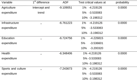
Table 2: Stationarity test (at 1st difference) results

Variable 1st difference ADF Test critical values at probability Agriculture

expenditure

Intercept and trend

-9.109051 1% -4.219126 5% -3.533083 10% -3.198312

0.0000

Infrastructure expenditure

,, -6.761223 1% -4.219126 5% -3.533083 10% -3.198312

0.0000

Education expenditure

,, -6.724756 1% -4.226815 5% -3.536601 10% -3.200320

0.0000

Health expenditure

,, -6.348406 1% -4.219126 5% -3.533083 10% -3.198312

0.0000

Sports and culture expenditure

,, -7.243673 1% -4.219126 5% -3.533083 10% -3.198312

0.0000

Source: constructed from the study data collected; Computed as per attached appendix 1

(22)

From the above table, all the variables are stationary since the ADF values are greater than the

corresponding critical values and the probability is less than 0.05 for all variables. Therefore the

data becomes stationary at first difference integrated of order 1 that is I(1).

Cointegration test

Because the variables are not stationary at level as evident from the unit root test results but are

integrated of order one, thus the linear combination of one or more of these variables might

exhibit a long run relationship. In order to capture the extent of cointegration among the

variables, the multivariate cointegration methodology proposed by (Johansen 1990) was

utilized. The results are shown in table 3 below.

Table 3: Johansen cointegration results

Hypothesized

No of CEs

Trace

statistics

Critical

value 0.05

p-value Maximum

Eigen

statistics

Critical

value0.05

p-value

None* 99.44733 95.75366 0.0272 42.49552 40.07757 0.0262 At most 1 56.95181 69.81889 0.3407 24.59660 33.87687 0.4128 At most 2 32.35521 47.85613 0.5925 14.00401 27.58434 0.8223 At most 3 18.35120 29.79707 0.5402 10.69113 21.13162 0.6780 At most 4 7.660073 15.49471 0.5024 7.483600 14.26460 0.4336 At most 5 0.176473 3.841466 0.6744 0.176473 3.841466 0.6744

*denotes rejection of the hypothesis at the 0.05 significance level

Source: constructed from the data collected; Computed as per attached appendix 2

From the above table, both trace statistics and maximum Eigen value test revealed one

cointegrating equation at 5% level of significance. The null hypothesis of no cointegration

among the variables was rejected at none since the p value was less than 0.05 in both tests.

This result therefore confirmed that there is a long run relationship between government

expenditure variables that is expenditure on education, infrastructure, agriculture, health and

sports and culture and economic growth.

Nevertheless, the cointegration result did not point the direction of the long-run

relationship between variables. Since there was evidence of cointegration, this confirmed the

existence of causality from GDP growth rate to government expenditure, or vice versa, or both.

Therefore, the next step was to carry out Granger-causality tests to determine the direction of

(23)

Licensed under Creative Common Page 130 VAR diagnostic tests

Prior to carrying out causality test, diagnostic tests were carried out in order to determine the

appropriate VAR model free from spurious VAR estimation results. The diagnostic tests carried

out included normality (Jarque-Bera test), autoregressive conditional heteroscedasticity(ARCH

LM test), and serial correlation (Breusch-Godfrey serial correlation LM test).The results are

presented in table 4 below.

Table 4: Diagnostic tests

Test F-statistics p-value

Normality: Jarque-Bera statistic 2.234339 0.327205

Serial correlation: Breusch-Godfrey serial correlation LM test 0.004138 0.9491 Autoregressive conditional heteroscedasticity: ARCH LM test 0.176053 0.6773

Source: constructed from the study data; Computed as per attached appendix 4

In normality test, null hypothesis of presence of normality was not rejected since the p-value is

greater than 5%.This confirmed that the data is normally distributed. For serial correlation test,

the null hypothesis of no serial correlation between the variables was not rejected since the

p-value is greater than 5% as shown in the table. Lastly the null hypothesis of no

heteroscedasticity was not rejected too because the p-value is greater than 5% as shown in the

table.

Therefore the diagnostic tests indicate that the residuals are normally distributed,

homoscedastic and serially uncorrelated.

Granger causality test

Granger causality is a technique for searching the direction of causation between variables after

the existence of cointegration (Kalyoncu & Yucel 2006). Cointegration results indicated a long run

relationship between the variables but did not indicate the direction of causation. Granger

causality test with various lags was carried out using pairwise granger causality criterion (table 5).

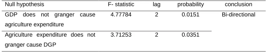
Table 5: Granger causality test

Null hypothesis F- statistic lag probability conclusion GDP does not granger cause

agriculture expenditure

4.77784 2 0.0151 Bi-directional

Agriculture expenditure does not granger cause DGP

(24)

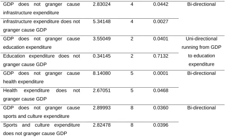
Licensed under Creative Common Page 131 GDP does not granger cause

infrastructure expenditure

infrastructure expenditure does not granger cause GDP

5.34148 4 0.0027

GDP does not granger cause education expenditure

3.55049 2 0.0401 Uni-directional running from GDP

to education expenditure Education expenditure does not

granger cause GDP

0.34145 2 0.7132

GDP does not granger cause health expenditure

Health expenditure does not granger cause GDP

2.67051 5 0.0468

GDP does not granger cause sports and culture expenditure

Sports and culture expenditure does not granger cause GDP

2.82478 8 0.0396

The granger causality test results revealed that there was bi-directional causality between

government expenditure on agriculture, infrastructure, health and sports and culture and

economic growth. The p- values for these variables are less than 5% hence the null hypothesis

was rejected. This means that these set of variables predicted each other and hence could be

on either side of the equation, (either as dependent or as an independent variable). These

results are consistent with the results of Maingi (2010).Education expenditure had a

unidirectional causality on economic growth.GDP granger causes education expenditure. These

findings confirm the use of VAR model given that there was directional causality between

economic growth and government expenditure components under the study.

From these results, there was a feedback effect between government expenditure

components and GDP growth rate, which supported the Wagner’s hypothesis that states that

increase in GDP causes growth in the government expenditure, and the Keynesian hypothesis

that states that increase in government expenditure causes GDP to increase. This suggests that

allocation of government resources should be designed carefully in order to spur economic

growth of the country.

Impulse response function

The impulse response function traced the effects of one standard deviation shock on a variable

on its own and on the other variables. The vertical axis shows the deviation from the baseline

(25)

level of the target variable in response to a one standard deviation shock of the independent

variable (Kigabo, et al.2015).

The specific objectives of this study were to analyze the effects of government

expenditure on various sectors on economic growth. The results were depicted by the following

response functions of GDP and the various government sectors

The effect of agriculture expenditure on GDP

The effect of a one standard deviation shock to agriculture expenditure on GDP is shown in the

figure 4 below.

Figure 4: effect of agriculture expenditure on GDP

There were fluctuations on the effects of agriculture expenditure on GDP throughout the study

period though the variations were positive (blue line trend) showing that agriculture expenditure

was significant in stimulating economic growth. There was a positive effect on GDP incase of a

one standard deviation shock in agriculture expenditure. This could be due to the fact that

increased agriculture expenditure improves the total agricultural output which increases

aggregate domestic consumption and export earnings which adds to the GDP.Improved

methods of farming through provision of quality seeds to farmers, fertilizer provision and

bringing more land under agriculture could have necessitated this outcome. The results are

similar to those of Abbas & Abdul (2016). They also found a positive relationship between

agriculture expenditure and economic growth in Pakistan.

-80,000 -40,000 0 40,000 80,000 120,000

1 2 3 4 5 6 7 8 9 10

(26)

Licensed under Creative Common Page 133 The effect of infrastructure expenditure on GDP

The effect of a one standard deviation shock to infrastructure expenditure on GDP is shown in

the figure 5 below.

Figure 5: effect of infrastructure expenditure on GDP

The effects of infrastructure on economic growth remained fairly stable on the negative side

throughout the study period exhibiting a decreasing trend initially and increasing trend from the

5th financial year as shown by the blue line below the base line in the above figure. This shows

that infrastructure expenditure had a negative effect on GDP within the study period. A one

standard deviation shock of infrastructure expenditure impacted negatively on economic growth.

This could be due to high expenditure on salaries and wages incurred on foreign firms given the

tenders initially since Rwanda had shortage of skilled manpower on construction of roads and

communication networking initially. This led to high capital outflow which could have impacted

negatively on economic growth. The steady rise in the effects can be explained by the fact that

Rwanda has improved her manpower and this has reduced the capital outflow though still not

enough to foster positive effects.

Effect of education expenditure on GDP

The effect of a one standard deviation shock to education expenditure on GDP is shown in the

figure 6 below.

-80,000 -40,000 0 40,000 80,000 120,000

1 2 3 4 5 6 7 8 9 10

(27)

Figure 6: effect of education expenditure on GDP

The effects of education expenditure on GDP remained positive for the entire period as shown

by the blue line in the above figure. A one standard deviation shock of education expenditure

had a positive effect on GDP. Education expenditure contributed greatly to economic growth

within the study period.

There were fluctuations on the effects but they generally exhibited an increasing trend

with time depicted by increased gap between the baseline and the blue line.

This trend could be attributed to the increased skilled labour force (human capital) with

time needed in the industries leading to increased efficiency in production hence increased total

output. This could have been achieved by carrying out awareness programmes on education,

expansion of learning institutions right from primary to university, provision of appropriate

physical infrastructure in schools, provision of high skilled manpower which ultimately increases

the marginal productivity of labour, introducing fee guidelines in the learning institutions and

finally increased number of government sponsored students to higher learning institutions. All

these factors led to increased enrolment rate in the learning institutions creating a pool of

skilled manpower required in both public and private sectors leading to increased GDP. The

results are consistent with those of Mekdad (2014) who also found a positive relationship

between education expenditure and economic growth in Algeria.

Effect of health expenditure on GDP

The effect of a one standard deviation shock to health expenditure on GDP is shown in the

figure 7 in the next page.

-80,000 -40,000 0 40,000 80,000 120,000

1 2 3 4 5 6 7 8 9 10

(28)

Figure 7: effect of health expenditure on GDP

The effects of a one standard deviation shock of health expenditure on GDP had an increasing

trend up to the fifth financial year, a decreasing trend after up to eighth financial year then a rise

and fall in the last two years. The effects were otherwise positive for the entire study period

depicted by the blue line being on the positive side of the base line.

This phenomenon could be due to the fact that health expenditure by the government

raises the health status and productivity of the people, thereby promoting economic growth. The

increased expectation of a longer life could affect the intertemporal discount rate and therefore

savings. Increased health expenditure could increase the participation of women in the labour

market, and affect fertility, which has effect on demographic transition and therefore on the

economy. Further, government investments on buildings of hospitals represent expenditure on

the core functions and therefore are expected to have a positive effect on the economy.

Effect of sports and culture expenditure on GDP

The effect of a one standard deviation shock to sports and culture expenditure on GDP is shown

in the figure below.

-80,000 -40,000 0 40,000 80,000 120,000

1 2 3 4 5 6 7 8 9 10

(29)

Figure 8: effect of sports and culture expenditure on GDP

The effect of a one standard deviation shock of sports and culture on economic growth was

negative initially, became positive shortly then dropped again for some time till the 6th financial

year before rising again. Generally there was fluctuation in the effects on both sides of the

baseline for the entire period. This shows that sports and culture expenditure had mixed effects

on economic growth.

The positive effects could be attributed to expansion of tourist sites and increased

expenditure on promotion of sports activities which saw more Rwandese playing in foreign clubs

which brings in foreign earnings for the country. Expansion of tourist sites and culture attracted

more tourists hence increased foreign earnings. The negative effects could be attributed to low

foreign earnings from tourism sector.

Variance decomposition analysis

This is an alternative method to analyzing the effects of shocks of government expenditure to

GDP. This technique determined how much of the forecast error variance for any variable in the

system was explained by innovations to each explanatory variable over a series of time horizon

(Enders, 1995). The own series shocks explained most of the error variance, although the shock

also affected other variables in the system.

-80,000 -40,000

0 40,00 0 80,00 0 120,00 0

1 2 3 4 5 6 7 8 9 1

(30)

Table 6: Variance Decomposition of GDP

Period S.E. Agriculture Education GDP Infrastructure Health Sports