ScholarlyCommons
Publicly Accessible Penn Dissertations
1-1-2014
Discovery of the Higgs Boson, Measurements of its
Production, and a Search for Higgs Boson Pair
Production
James C. Saxon
University of Pennsylvania, james.saxon@gmail.com
Follow this and additional works at:
http://repository.upenn.edu/edissertations
Part of the
Elementary Particles and Fields and String Theory Commons
This paper is posted at ScholarlyCommons.http://repository.upenn.edu/edissertations/1433 For more information, please contactlibraryrepository@pobox.upenn.edu.
Recommended Citation
Saxon, James C., "Discovery of the Higgs Boson, Measurements of its Production, and a Search for Higgs Boson Pair Production"
(2014).Publicly Accessible Penn Dissertations. 1433.
Search for Higgs Boson Pair Production
Abstract
This document chronicles the discovery of the Higgs boson and early measurements in the diphoton decay
channel. Particular attention is paid to photon identification, to the coupling of the Higgs to the vector bosons,
and to differential cross sections of the Higgs boson. As these measurements yielded good agreement to the
predictions of the Standard Model, an additional search is performed, for Higgs boson pair production in the
γγbb final state. The dataset used represents 5/fb of proton- proton collisions at sqrt(s) = 7 TeV and 20/fb of
collisions at sqrt(s) = 8 TeV, recorded by the ATLAS experiment at CERN's Large Hadron Collider in 2011
and 2012.
Degree Type
Dissertation
Degree Name
Doctor of Philosophy (PhD)
Graduate Group
Physics & Astronomy
First Advisor
Hugh H. Williams
Keywords
couplings, differential cross sections, dihiggs, higgs, pair production, photon
Subject Categories
Elementary Particles and Fields and String Theory
Measurements of its Production,
and a Search for Higgs Boson Pair Production
James C. Saxon
a dissertation
in
Physics and Astronomy
Presented to the Faculties of the University of Pennsylvania
in
Partial Fulfillment of the Requirements for the
Degree of Doctor of Philosophy
2014
Hugh H. Williams, Professor, Physics
Supervisor of Dissertation
Marija Drndic, Professor, Physics
Graduate Group Chairperson
Dissertation Committee
Eugene Beier, Professor, Physics
I. Joseph Kroll, Professor, Physics
Elliot Lipeles, Associate Professor, Physics
and a Search for Higgs Boson Pair Production
I began working on the ATLAS experiment for the University of Pennsylvania more than eleven years ago, at the tender age of fifteen. My time on ATLAS therefore coincides not only with my formation as a physicist but also very substantially with my development as a person. I am overwhelmed to reflect on the impact that the Penn group and the ATLAS collaboration have had on me. I am grateful for the camaraderie of barbecues, dinners, Bond flics, and discussions that continued through years. I am grateful for the technical skills, the intellectual challenges, and the infectious passion that so many people have shared with me. To all those who supervised me, helped me, and taught me – thank you for inviting me to join in this adventure.
Rick Van Berg gave me my very first job at Penn, and our innumerable discussions over the intervening decade have enriched me both intellectually and personally. Brig Williams is a true gentleman – sharp as a tack, but gracious and genuinely kind. He has cultivated the Penn group with wisdom and tenacity. He has been unfailingly accessible and supportive, and led with high expectations and a long leash. I could not have asked for a better advisor. All of the professors in the ATLAS group – Elliot Lipeles, Joe Kroll, and Evelyn Thomson – assisted in supervising me, and it was a blessing to have such a collaborative team. I am also grateful to the non-ATLAS reviewers of my thesis – Mark Trodden and Gene Beier.
Mike Hance, John Alison, and Dominick Olivito set the bar for Penn students at CERN – and they set it high. Mike was incredibly generous with his phenomenal expertise with the TRT and with
photons. John defined, more than anyone, theesprit de corps that made the group so successful.
He is one of the most intense intellectuals that I have ever met, and I look forward to our continued collaboration in Chicago. Dominick turned the TRT into one of the smoothest functioning detectors on ATLAS. He personally watched over my development and put up with me with greater patience than anyone should have had to – in commissioning the TRT, refining the DAQ, and preparing physics analysis.
Special thanks goes to my other house-mates who magnanimously put up with ‘a boy singing’: Kurt Brendlinger and Alex Tuna at Taney, and Chris Lester and Jon Stahlman (formerly of Taney). Kurt has been a great, long-suffering friend since about the seventh grade, and hopefully for a long time to come (though perhaps with less suffering). He was also an invaluable homework buddy during my first two years at Penn. Tuna sprinted through his classes but was always happy to help me slug through. My life would have fewer cats without him. Lester is a mensch and a great thinker, and helped me hold on to scraps of sanity in the months that we overlapped at Hautains. Stahlman bore a great piece of the responsibility for the TRT during my time at CERN, and was a stalwart champion of the BBQs for several years.
The Penn Army (and honorary Penn Army) was a dynamic, fun-loving, hard-working crew, I am
much the richer for having grown up with all of you, and I consider myself very fortunate. You have been incredible colleagues and wonderful friends. I look forward to watching the group continue to evolve and grow – both as current members move on to new posts and projects, and as rising students take the group to ever greater heights.
My time on the TRT stretched over its construction, commissioning, and Run I operations. Ole Røhne, Franck Martin, Jack Fowler, Ben LeGeyt (and of course, Mike and Dominick) ensured the successful completion of the detector, and watched over me in my first summers at CERN. Christoph Rembser is a model of good leadership in large collaborations, shouldering bureaucracies, supporting a strong community, and responding to every request with great humour. Anatoli Romaniouk’s long-term care for details has been fundamental to achieving and maintaining the high performance of the TRT. Andrey Loginov was always there to help clear the way for us to ‘just work.’ Zbyszek Hajduk, Jola Olszowska, Elzbieta Banas of the Krakow group kept the TRT electronics running and the detector safe, and supported us every step of the way. Of my home in the DAQ crew, it was a great privilege to work with Mike, Dominick, Peter Wagner, Jon Stahlman, Sarah Heim, Ximo Poveda, Paul Keener, Mitch Newcomer, Godwin Mayers, and Rick Van Berg – and now Chris Meyer, Khilesh Mistry, Bijan Haney, Tony Thompson and Leigh Schaefer.
My first analysis work was in the e/γ group. Fabrice Hubaut, Andrea Bocci, Marco Delmastro,
and Marcos Jimenez provided good-natured and level-headed leadership and taught me everything that I know about photons (that I didn’t learn from Mike and Brig!). It was a pleasure for me to work with Kun Liu and Evgeny Soldatov on the efficiency measurements in 2011 and 2012. Leonardo Carminati was a great ally in preparing cuts for 2012 data.
The h → γγ working group managed to be a functional, pleasant environment for a young
student, despite the enormous pressures at the time of the discovery. The group conveners played an important role in maintaining this good environment, and helped to make my time in the group exciting and enjoyable. Marc Escalier did a phenomenal job, defining the analysis in very early data, and shepherding it through an ‘exciting’ moment in April 2011. I am very grateful to Junichi Tanaka, Kerstin Tackmann, Krisztian Peters, Nicolas Berger, and Sandrine Laplace, who allowed me opportunities to stretch my wings and really learn to do analysis. Nicolas helped me with patience, kindness, and energy well beyond any reasonable expectations, to understand statistics.
The Orsay group gave me a home away from home in 2013, and afforded me the detailed, expert attention that has made their own group such a powerhouse. My especial thanks go to Louis Fayard, Estelle Scifo, Marc Escalier, and Nansi Andari, who welcomed me several times at LAL. The Wisconsin group were also frequent and diligent collaborators; I particularly want to thank Andrew Hard, Hongtao Yang, and Haichen Wang. In studying missing energy and preparing couplings analyses, Bruce Melado, Amanda Kruse, and Elisabeth Petit were a pleasure to work with. Within
the missing energy group, my thanks go to the Milan team, and to Irene Vichou who made theE/T
work, and answered my endless questions to make sure that the definitions used for h→ γγ were
correct and optimal.
One of my greatest pleasures in my time on ATLAS was working with Dag Gillberg and Florian Bernlochner on the differential cross sections conference note. They are fast, smart, insightful, fun, and basically just the best collaborators I could imagine working with. My thanks go to the full differential cross sections team, that produced a beautiful result on a very short time frame, and to our editorial board (Fabrice and Mike, again, as well as Mark Sutton) who helped us to get it out in a timely manner.
was an abiding pleasure to work and chat with him; I look forward to our continued collaboration in Illinois. Leandro Nisati and our entire editorial board mustered quite a force in reviewing the analysis and pushing it through to approval.
Among physicists, my last thanks go Chicago, for inviting me to continue with them on the next leg of this journey. It is an awesome team that I am extremely excited to join!
My parents granted me tremendous independence at a young age, but supported me when I needed them, and helped me to think through and deal with my decisions. They set for me a rich example of deliberate, practical morality and decency.
Discovery of the Higgs Boson,
Measurements of its Production,
and a Search for Higgs Boson Pair Production
James C. Saxon
Hugh H. Williams
This document chronicles the discovery of the Higgs boson and early measurements in the
dipho-ton decay channel. Particular attention is paid to phodipho-ton identification, to the coupling of the Higgs
to the vector bosons, and to differential cross sections of the Higgs boson. As these measurements
yielded good agreement to the predictions of the Standard Model, an additional search is performed,
for Higgs boson pair production in theγγbbfinal state. The dataset used represents 5 fb-1of
proton-proton collisions at √s= 7 TeV and 20 fb-1 of collisions at √s = 8 TeV, recorded by the ATLAS
experiment at CERN’s Large Hadron Collider in 2011 and 2012.
Acknowledgements iii
Abstract vi
Contents vii
List of Tables xiv
List of Figures xv
1 Introduction 1
2 Theoretical Context 4
2.1 The Standard Model . . . 4
2.2 The Higgs Mechanism . . . 5
2.3 Theoretical and Experimental Constraints . . . 7
2.4 Higgs Production at the LHC . . . 9
2.5 Higgs Boson Pair Production . . . 13
2.5.1 Standard Model Production . . . 13
2.5.2 Production Beyond the Standard Model . . . 14
2.5.2.1 Resonant Production . . . 14
2.5.2.2 Non-Resonant Production . . . 15
3 Experimental Apparatus 16 3.1 The Large Hadron Collider . . . 16
3.2 The ATLAS Detector . . . 18
3.2.1 Coordinate System . . . 19
3.2.2 Detector Overview . . . 20
3.2.2.1 Inner Detector . . . 20
3.2.2.2 Calorimetry . . . 23
3.2.2.3 Muon Detectors. . . 26
3.2.2.4 Trigger System . . . 27
4 Photon Reconstruction and Identification 28 4.1 Photon Reconstruction . . . 28
4.2 Photon Calibration . . . 30
4.2.1 Calculation of Cell Energies . . . 30
4.2.2 Corrected Cluster Energy . . . 31
4.2.3 Residual Calibration from Data . . . 32
4.2.4 Conversion Correction . . . 33
4.3 Photon Identification . . . 33
4.3.1 IsEM Variables . . . 34
4.3.2 ‘Fudge Factors’ . . . 37
4.3.3 Cuts-Based Identification and Trigger . . . 39
4.3.4 Neural Network Identification for 2011 Data . . . 40
4.3.4.1 Validation of Input (isEM) Distributions . . . 41
4.3.4.3 Results . . . 48
4.3.4.4 Efficiencies from Data, and Systematics . . . 51
4.3.4.5 Additional Studies . . . 52
4.3.5 Cuts-Based Optimization for 2012 Data . . . 56
4.3.5.1 Studies of Potential Systematics . . . 56
4.3.5.2 ‘Landmark’ Cuts Menus . . . 58
4.3.5.3 Tools for Refining Menus . . . 59
4.3.5.4 Early Data: New Optimal Filtering Coefficients . . . 62
4.3.6 Measurements of Identification Efficiency . . . 63
4.4 Photon Isolation . . . 63
4.4.1 Calorimeter Isolation . . . 64
4.4.2 Track Isolation . . . 65
5 Discovery of the Higgs Boson 66 5.1 Event Selection . . . 67
5.2 Simulation . . . 69
5.2.1 Signal . . . 69
5.2.1.1 Corrections to the Signal Monte Carlo . . . 70
5.2.2 Background Simulation . . . 72
5.3 Modelling . . . 72
5.3.1 Signal . . . 73
5.3.2 Background Shape and ‘Spurious Signal’ . . . 73
5.4 Categorization . . . 75
5.5 Overview of Uncertainties . . . 77
5.5.2 Uncertainties on the Mass Shape . . . 79
5.5.3 Migration Uncertainties . . . 79
5.6 Statistical Model and Mechanics . . . 79
5.7 Discovery of the Higgs Boson . . . 82
6 Coupling Measurements 84 6.1 Object Definitions . . . 84
6.2 Categories . . . 86
6.2.1 Lepton Category . . . 86
6.2.2 Missing Energy Category . . . 87
6.2.2.1 Reconstruction and Alterations to the Default Definition . . . 87
6.2.2.2 Confronting Pileup . . . 89
6.2.2.3 Systematic Uncertainties . . . 91
6.2.3 Other Categories . . . 93
6.2.3.1 HadronicV h. . . 93
6.2.3.2 VBF Binary Decision Tree. . . 93
6.2.3.3 Addendum: Recent Additions and Continued Work . . . 93
6.3 Results . . . 94
6.3.1 Combinations with other Channels . . . 95
7 Differential Cross Sections 98 7.1 Selection Requirements . . . 99
7.1.1 Reconstructed Events and Data . . . 99
7.1.2 Truth-Level Events: Definition of the Fiducial Region . . . 100
7.1.2.1 Definition of the Fiducial Region . . . 100
7.1.2.3 Jet Definition . . . 102
7.2 Signal Extraction . . . 102
7.2.1 Binning of the Observables . . . 102
7.2.2 Fit Procedure and Yield Extraction . . . 103
7.3 Unfolding Procedure . . . 104
7.3.1 Correction Factors . . . 104
7.3.2 Alternative Method: Bayesian Unfolding . . . 106
7.4 Systematic Uncertainties . . . 107
7.4.1 Shape and Modelling Uncertainties . . . 108
7.4.2 Uncertainties Shared with Previous Results . . . 108
7.4.3 Uncertainties on the correction factors, from the choice of model . . . 109
7.4.4 Summary of the Uncertainties . . . 111
7.5 Theoretical Predictions . . . 111
7.5.1 Errors on Theoretical Predictions . . . 113
7.6 Results and Interpretation . . . 114
8 Pair Production 120 8.1 Simulated Samples . . . 121
8.1.1 SM Higgs Boson Pair Production . . . 121
8.1.2 Narrow-Width, Gluon-Initiated Scalar . . . 121
8.1.3 Samples for Background Studies . . . 124
8.2 Event Selection and its Optimization . . . 124
8.2.1 Optimization . . . 125
8.2.1.1 Jet Momentum Corrections . . . 125
8.2.1.3 Mass Constraint . . . 129
8.2.2 Event Selection . . . 130
8.3 Background Studies . . . 131
8.3.1 Non-Resonant Backgrounds . . . 131
8.3.1.1 Sideband Fit in Data . . . 131
8.3.1.2 Monte Carlo: Composition . . . 133
8.3.2 Backgrounds from Single Higgs Boson Production . . . 134
8.4 Analysis Strategy . . . 134
8.4.1 Non-Resonant Production . . . 135
8.4.2 Resonant Production . . . 136
8.5 Systematic Uncertainties . . . 139
8.6 Results and Interpretations . . . 141
9 Conclusions 144 Appendices 146 A IsEM Distributions ofZ →``γ Radiative Decays . . . 147
B Z→eeEfficiencies in Data and Monte Carlo . . . 148
C Higgs Decays tof f γ . . . 149
D Missing Energy Performance for Coupling Studies . . . 150
D.1 Impact of the Redefinition of the Missing Energy . . . 150
D.2 Studies of the ‘Soft Track Vertex Fraction’ . . . 150
E Additional Variables for aEmiss T -Only Category . . . 153
F Missing Energy Systematics for Coupling Studies . . . 154
G Migration Uncertainties for the Coupling Analysis . . . 155
I Differential Cross Sections: Alternative Theoretical Predictions . . . 164
J Simulation Samples for the Higgs Pair Production Search . . . 165
K Cuts Optimization for Higgs Pair Production . . . 169
L Additional Control Regions and Fits for Higgs Pair Production . . . 170
2.1 SM cross sections of Higgs boson (pair) production . . . 9
4.1 Cluster sizes for electrons and photons . . . 30
4.2 Discriminant Cuts for Loose Photon Identification . . . 40
4.3 Discriminant Cuts for Tight Photon Identification . . . 57
6.1 Estimated impact of the missing energy category on themuV H measuremrent . . . 90
6.2 Various electron ambiguity resolution definitions, for theEmiss T category . . . 91
6.3 Uncertainties on the categorization of events due to the missing energy . . . 92
7.1 Extracted differential cross sections . . . 99
7.2 Expected events by production mode, for the differential cross section measurement . . 101
7.3 Probability of theχ2between measured differential distributions and SM predictions . . 114
8.1 Fitted resolutions for various pT corrections. . . 126
8.2 Optimization of b-tagging for Higgs pair production . . . 129
8.3 Cut Flow and Event Yields . . . 131
8.4 Background processes and contributions . . . 133
8.5 SM single Higgs boson contributions to the non-resonant pair production search . . . . 134
8.6 Summary of systematics uncertainties for pair production searches . . . 142
F.1 Unabridged systematics on missing energy in the search for V hand t¯thin the h→γγ search . . . 154
G.2 Migration uncertainties for the couplings analysis . . . 155
H.1 Summary forNjets differential cross section . . . 157
H.2 Summary for|yγγ |differential cross section . . . 158
H.3 Summary forpγγT differential cross section . . . 159
H.4 Summary for|cosθ∗|differential cross section . . . 160
H.5 Summary forpjT1 differential cross section . . . 161
H.6 Summary for ∆ϕjj differential cross section . . . 162
H.7 Summary forpγγjjT differential cross section . . . 163
2.1 The ‘Mexican hat’ potential . . . 6
2.2 Constraints on the Higgs boson mass before its observation. . . 8
2.3 Standard Model Higgs boson production diagrams. . . 11
2.4 Cross sections and branching ratios of the SM Higgs boson . . . 11
2.5 Diagrams of the decay modes of the SM Higgs boson. . . 11
2.6 Dihiggs production diagrams . . . 13
2.7 Cross section times branching ratio for a resonant dihiggs production in a 2HDM . . . 15
3.1 The LHC injection complex and the data it produced . . . 18
3.2 Schematic of the inner detector . . . 20
3.3 Schematic of the liquid argon calorimeter . . . 24
4.1 Schematic of photon trigger, reconstruction, and identification . . . 29
4.2 Schematic diagram of a calorimeter cluster . . . 31
4.3 Schematic of isEM variables . . . 34
4.4 ‘IsEM’ variables for unconverted photons . . . 36
4.5 ‘IsEM’ variables for converted photons . . . 37
4.6 Illustration of the fudging procedure . . . 39
4.7 Comparison of isEM variables from the leading (di)photon . . . 44
4.8 Photon ID efficiency v. jet rejection for various MVA methods . . . 45
4.9 Schematic of the neural network, and example output . . . 47
4.10 Photon ID efficiencies in MC and fromZ →``γ decays . . . 49
4.11 Purity measurement of events selected in theh→γγ analysis with NN andTight PID 51 4.12 Efficiencies of the neural network, measured in data . . . 53
4.13 Difference in photon ID efficiency with nominal and distorted geometries . . . 54
4.14 Monte Carlo and data efficiencies for electrons to pass neural network andtight identifi-cation . . . 55
4.15 Photon identification efficiency as a function of the number of vertices per event . . . . 55
4.16 Degradation ofRϕ andRhad with pileup . . . 59
4.17 Examples of tight cuts suggested from TMVA simulated annealing . . . 60
4.18 N−1 Efficiencies compared for 2011 and 2012 cuts menus . . . 61
4.19 Example of the ‘microscopes’ used in optimizing individual cuts . . . 61
4.20 Efficiencies in simulation of candidate cuts menus . . . 62
4.21 Sketch of isolation variables . . . 64
5.1 Cartoon of the search for the Higgs boson in the diphoton channel . . . 67
5.2 Global signal fit example . . . 74
5.3 Schematic diagram of the spurious signal procedure, and an example . . . 75
5.4 Variables for categorization . . . 77
5.5 Diphoton invariant mass spectrum, used for discovery . . . 82
5.6 CLS exclusion andp0 fromh→γγ at the discovery . . . 83
5.7 Local probability of the no-Higgs boson hypothesis, for the ATLAS discovery. . . 83
6.1 Impact ofZ mass veto on the lepton category . . . 87
6.2 Emiss T Significance, and invariant mass in the ‘ETmiss’ Category . . . 91
6.3 Expected composition of h→γγ ‘coupling categories’ by production mode . . . 94
6.4 Summary of combination of couplings analyses between all channels . . . 96
7.1 Deformation of the invariant mass spectrum for cuts on pγγT . . . 100
7.2 Example fits of the diphoton invariant mass, for nJets= 1 andnJets= 2 . . . 104
7.3 Correction factors for differential cross sections . . . 105
7.4 ‘Purities’ for events to be reconstructed in the ‘right’ bin, for the differential cross sections 106 7.5 Examples of Bayesian iterative unfolding . . . 107
7.6 Combined uncertainties on the differential cross sections for pγγT ,|yγγ |,|cosθ∗|,N jets . . 112
7.7 Combined uncertainties on the differential cross sections: pjT1, ∆ϕjj, and pγγjjT . . . 113
7.8 Fiducial differential cross sections of the Higgs boson in pγγT ,|yγγ |,|cosθ∗|, andN jets . . 117
7.9 Fiducial differential cross sections of the Higgs boson in pjT1, ∆ϕjj, hjjpt . . . 118
7.10 Jet veto distribution for Higgs boson production . . . 119
8.1 Kinematics of the Higgs pair production ‘heavy scalar’ (HS) and SMhhbenchmarks . 122 8.2 Di-jet mass with various corrections . . . 126
8.3 Optimization of theb pT cuts . . . 128
8.4 Optimization of themb¯b cuts on the Higgs pair production search . . . . 128
8.5 Four-object mass, with and withoutmb¯b constraint . . . . 129
8.6 Efficiency of the inclusive selection, for resonance models . . . 130
8.7 Sideband fit of the pair production signal region, with control regions . . . 132
8.8 Fit ofmγγ in the search for non-resonant pair production . . . . 136
8.9 Cuts for 95%mγγb¯b acceptance . . . 137
8.10 Comparison of Landau fits in data sidebands and MC . . . 138
8.11 Signal region of the search for resonant pair production, inmγγb¯b . . . . 139
8.12 Limit on resonant Higgs boson pair production . . . 143
A.1 IsEM distributions from radiativeZ decays in 2011 data . . . 147
B.1 Photon identification efficiencies evaluated onZ→eeelectrons . . . 148
C.1 Dalitz diagram and mass spectrum off f pairs . . . 149
D.1 Comparison of treatment of photons with differentEmiss T algorithms . . . 150
D.2 Resolution of nominal RefFinal and STVFEmiss T usinggghevents . . . 151
D.3 Tails of STVF, and performance as a function ofpγγT . . . 152
E.1 Additional discriminating variables for aEmiss T -only category . . . 153
I.1 Leading parton radiation in Higgs boson production, compared to NNLO predictions . 164 I.2 Differential cross sections for Njets andσNjets=i/σNjets≥i, using Stewart-Tackmann . . . 164
J.1 Kinematics of generated SM hh, compared to theory . . . 165
J.3 Kinematic distributions for 2HDM production, fromMadGraphandPythia8. . . 167
J.4 Comparison of the single-tag control region in data and MC . . . 168
K.1 Optimization ofb pTcuts: additional signal models . . . 169
Introduction
The Standard Model of particle physics is a testament to the intensity of human curiosity and
an intellectual triumph. It describes three of the four known forces with astounding accuracy; it
integrates a century of experiments within an alternately elegant and ad hoc theory. Yet for five
decades its keystone was absent. This document describes the crowning achievement of the Standard
Model: the experimental observation of the Higgs boson.
In March 1984, the European Organization for Nuclear Research (CERN) and the European
Committee for Future Accelerators (ECFA) hosted a workshop in Lausanne, to consider proposals
for a ‘Large Hadron Collider in the LEP Tunnel.’ Twenty years had already passed since the Higgs
mechanism was first described [1–3]. The Standard Model described by Glashow, Weinberg, and
Salam had just been vindicated by the discovery of the W and Z vector bosons by the UA1 and
UA2 experiments at the Super Proton Synchrotron [4–7]. The participants in the 1984 workshop
concluded that ‘searching for the Higgs meson [sic.] as it appears in the standard model looks
difficult,’ and in particular that gluon fusion ‘does not seem to be a promising mechanism’ [8]. On
the other hand, supersymmetry was expected to be readily accessible.
By 1992 however, when the ATLAS and CMS Collaborations submitted Letters of Intent for
large, multi-purpose detectors on the LHC [9,10], the detector design parameters and the physics
case of the two experiments had swung decidedly in favor of the discovery potential of the Higgs
boson in the diphoton andZZ channels. The two experiments were approved in early 1997, and civil
engineering work began shortly thereafter. The ATLAS prototype detectors were first assembled in a
2003 test beam, and the experimental cavern was completed that year, 100 m below the Franco-Swiss
border. Installation of the 7000-ton, 13-story detector would continue for the next four years. LHC
collisions began in September 2008, but abruptly ended nine days later, when a faulty interconnect
between two superconducting magnets caused a quench and an explosion that destroyed several
magnets [11]. Data collection recommenced in 2009 and accelerated through 2011 and 2012, leading
to the discovery of the Higgs boson announced on July 4, 2012.
The diphoton andZZ decay channels were the two components to the initial Higgs observation
by ATLAS.1 The diphoton channel remains one of the most-important modes for the study of its
couplings. Its small branching fraction of just 0.2% is offset by a high selection efficiency of∼40%,
good mass resolution, and a relatively straightforward analysis strategy. This document chronicles
the discovery of the Higgs boson in this channel, and describes early measurements of its interactions.
It concentrates, naturally, on those topics to which the author made meaningful contributions:
. Chapters 2and 3briefly describe the theoretical context for the work, and present the Large
Hadron Collider and the ATLAS detector.
. Chapter 4 describes techniques for identifying photons showers and rejecting QCD
back-grounds. These methods were central to the Higgs discovery by ATLAS, which is discussed in
Chapter 5. That work was first published in Ref. [12].
. Following the discovery of a new particle, the task was to determine whether it behaved as the
SM Higgs boson. Two paths were open: (1) to check that the particle was indeed a scalar, or (2)
to measure whether its interactions with other particles scaled with their masses. The author
chose the second path. Chapter 6 therefore describes efforts to select events consistent with
Higgs bosons produced in association with a W or Z boson, and thereby isolate production
through theW W hand ZZhvertices. This work was an important part of the early ATLAS
paper on the Higgs couplings [13].
. As the early coupling and spin results agreed with the predictions of the SM within
experi-mental error, differential cross sections of Higgs boson production were extracted, to further
assess the compatibility of the new particle to the SM Higgs boson. These measurements are
described in Chapter 7 based on work first released in a conference note [14], for which the
author served as an editor.
. A search for Higgs boson pair production in the γγbbchannel, is described in Chapter8. The
cross section for this process is exceedingly small in the SM, but it is enhanced, resonantly or
non-resonantly, in a number of extensions to it. No significant discrepancy was found from the
null hypothesis, but this channel remains promising for Run II. A paper has been released,
also co-edited by the author [15].
Complementary measurements of mass, spin, and parity are summarized briefly, to present a fuller
picture of the consistency of the new particle to the SM Higgs boson. Measurements from and
Theoretical Context
A complete presentation of the Standard Model is beyond the scope of this document, and has
long been available from better-qualified authors [16,17]. The few details necessary to motivate this
work are included for completeness.
2.1
The Standard Model
The Standard Model of particle physics (SM) is a theoretical description of the elementary
particles that make up matter, and three of the four forces that govern their interactions. There are
three families of quarks and leptons, each with a left-handed doublet and two right-handed singlets:
u
d
L
, uR, dR and
ν
e−
L
, e−R, νR (2.1)
(The right-handed neutrinos need not exist, but appear in some models of neutrino masses.) Each of
the three forces is mediated by spin-1 bosons. The strong force (Quantum Chromodynamics, QCD)
is mediated by an octet of colored gluons, electromagnetism (Quantum Electrodynamics, QED) by
the photon, and the weak force by the W± and Z0 (after symmetry breaking). Together, these
forces and particles describe all familiar phenomena aside gravity.
Local gauge invariance is required for the renormalizability of the theory. The SM Lagrangian is
invariant under local transformations of the gauge groupSU(3)c×SU(2)L×U(1)Y, wherec refers
to color, Ldenotes the handedness of the SU(2) coupling, and Y refers to the weak hypercharge.
Local gauge invariance is preserved through the introduction of a covariant derivative, which in
turn implies the existence of the spin-1 gauge bosons. The structure functions of the underlying Lie
groups (the Lie Algebra), determine the form of the covariant derivative and the properties of the
gauge interaction.
The SM Lagrangian may be factored into four pieces:
LSM=Lgauge+Lf +Lϕ+LYukawa. (2.2)
‘Gauge’ includes the kinetic energies and (self-)interactions of the gauge bosons. Lf includes kinetic
energies of the fermions and, through the covariant derivative, their interactions with the gauge
bosons. Because the left-handed and right-handed fermions transform differently under SU(2)L, it
is impossible to directly write mass terms for them. Mass terms for the gauge bosons likem2G
µGµ
are not gauge invariant, and are similarly absent at this stage.
The bulk of this thesis focuses on tests of the second two terms in Equation2.2: the Higgs kinetic
terms and potential,Lϕ, and its interactions with the fermions,LYukawa. Without these terms, the
weak interaction would have infinite range, the fermions would be massless, and there would be no
Higgs boson.
2.2
The Higgs Mechanism
The ground state of a physical system need not preserve its intrinsic symmetries. For instance,
a heated magnet is rotationally symmetric, but ‘chooses’ a preferred direction when cool. In the
canonical example, the ‘Mexican hat potential’ of a complex fieldϕ
V (ϕ) =µ2 ϕ†ϕ+λ ϕ†ϕ2 (2.3)
is rotationally symmetric, but forµ2<0 andλ >0, its minimum lies in circle around the origin, with
Figure 2.1: The ‘Mexican hat’ potential canonically illustrates the principle of a spontaneously broken symmetry.
by choosing a point on that circle.
The Higgs mechanism uses spontaneous symmetry breaking to introduce both gauge boson and
fermion masses while respecting gauge invariance [1–3]. This is accomplished through the
introduc-tion of a doublet of scalar fieldsϕthat transforms underSU(2)L×U(1)Y, along with the (initially)
symmetric potentialV(ϕ) (Equation2.3). The LagrangianLϕ takes the form
Lϕ= (Dµϕ)†(Dµϕ)−µ2 ϕ†ϕ−λ ϕ†ϕ
2
, (2.4)
where the covariant derivative is (Dµϕ) = (∂µ+igτ·Wµ/2 +ig0Bµ/2)ϕ and Wi and B are the
gauge bosons associated toSU(2)L andU(1)Y respectively. The minimum of the potential is ν =
p
−µ2/λ, and is chosen to fall along the real part of the lower component ofϕ:
ϕ=√1 2
ϕ1+iϕ2
ϕ3+iϕ4
=⇒ ϕ0=
1
√
2 0
ν
. (2.5)
Usingϕ→ν+hto expand Equation2.4 around this minimum, and reorganizing theWi
µ and Bµ
as the familiarW± andZ0, yields
Lϕ= (∂µh)2/2 +m2WWµ+W−µ
1 + h
v
2
+m2ZZµZµ
1 + h
v
2
+µ
4
4λ+µ
2h2+λνh3+λ 4h
4. (2.6)
The gauge boson masses thus appear as couplings to the condensate of the Higgs potential. The
The degrees of freedom from the broken symmetry that would typically manifest as Goldstone bosons
are instead ‘eaten’ by the longitudinal polarization of theW and Z. The combination ofW3 and
B corresponding to the photon does not acquire a mass andU(1)EM remains as a symmetry of the
theory. Note that the Higgs boson’s own mass has also appeared: mh=
p
−2µ2=√2λν.
The fermion masses appear in a similar way: as a (three-point) Yukawa interaction with the vev
of the Higgs field. Before symmetry breaking, this is
LYukawa=−
X
families
ΓumnqmLϕu˜ nR+ ΓdmnqmLϕenR+ Γemn`mLϕenR+ Γνmn`mLϕν˜ nR (2.7)
where the conjugate form of the Higgs field breaks to ˜ϕ= (v+h,0)/√2 and the fermion fields are
the weak (not mass) eigenstates. The matrices Γi
mnare totally arbitrary, but will be proportional to
a (non-diagonal) mass matrix. After symmetry breaking, these terms are again reexpressed around
the vev leading to terms like Γe
mn`mL(ν+h)enR/
√
2. Suggestively definingMmn≡νΓmn/
√
2 yields
instead
LYukawa=−`mLMmne (1 +gh/2mW)enR/
√
2 +· · ·. (2.8)
Because the Higgs boson and the vev of the field are introduced together in the Yukawa interaction,
the resultant masses of the fermions are proportional to the strength of their coupling with the Higgs
boson.
2.3
Theoretical and Experimental Constraints
In tandem with precision electroweak and top quark measurements, the theoretical framework
of the Standard Model restricted the values that the Higgs boson mass could take and provided
indirect measurements of its value, before its direct observation. Both LEP and the Tevatron also
searched directly for the Higgs without finding it, and set exclusions.
Three fundamental theoretical limits may be considered. A first consideration provides both a
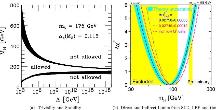
Figure 2: Summary of the uncertainties connected to the bounds onMH. The upper
solid area indicates the sum of theoretical uncertainties in theMH upper bound for
mt = 175 GeV [12]. The upper edge corresponds to Higgs masses for which the
SM Higgs sector ceases to be meaningful at scale Λ (see text), and the lower edge
indicates a value ofMH for which perturbation theory is certainly expected to be
reliable at scale Λ. The lower solid area represents the theoretical uncertaintites in
theMH lower bounds derived from stability requirements [9, 10, 11] usingmt= 175
GeV andαs= 0.118.
Looking at Fig. 2 we conclude that a SM Higgs mass in the range of 160 to
170 GeV results in a SM renormalisation-group behavior which is perturbative and
well-behaved up to the Planck scale ΛP l!1019GeV.
The remaining experimental uncertainty due to the top quark mass is not
rep-resented here and can be found in [9, 10, 11] and [12] for lower and upper bound,
respectively. In particular, the resultmt= 175±6 GeV leads to an upper bound
MH<180±4±5 GeV if Λ = 1019GeV, (4)
the first error indicating the theoretical uncertainty, the second error reflecting the
residualmtdependence [12].
5
(a) Triviality and Stability
0 1 2 3 4 5 6
100
30 300
m
H[
GeV
]
!"
2
Excluded Preliminary
!#had =
!#(5)
0.02758±0.00035 0.02749±0.00012
incl. low Q2 data
Theory uncertainty
July 2010 mLimit = 158 GeV
Figure 5: ∆χ2=χ2−χ2
minvs.mHcurve. The line is the result of the fit using all high-Q2data (last
column of Table 2); the band represents an estimate of the theoretical error due to missing higher
order corrections. The vertical band shows the 95% CL exclusion limit onmHfrom the direct searches
at LEP-II (up to 114 GeV) and the Tevatron (158 GeV to 175 GeV). The dashed curve is the result
obtained using the evaluation of ∆α(5)had(m2Z) from Reference 96. The dotted curve corresponds to a
fit including also the low-Q2data from Table 3.
12
(b) Direct and Indirect Limits from SLD, LEP and the Tevatron
Figure 2.2: Constraints on the Higgs boson mass before its observation.
Higgs to exist. Ifmhis too large, or if it is removed from the theory, the amplitude for longitudinally
polarized W W scattering grows linearly with s. This leads to a violation of unitarity at the TeV
scale, sosomething must break electroweak symmetry.
Two other limits take advantage of the running ofλ=m2
h/2ν2 with Q2, and yield results that
depend on an upper range of applicability of the theory, Λ. The first, triviality, refers to the ‘Landau
pole’ that arises inλ Q2at large m
h: the self-couplingλcannot diverge where the theory is valid.
This leads to a limit ofmh<140 GeV, if the theory is valid up to the Planck scale, ormh.650 GeV
if the theory is valid up to Λ = 1.5 TeV [16,18]. A lower bound comes from requiring λ Q2>0,
which is necessary for the stability of the vacuum. The resultant limits range from 85 GeV at
Λ = 1.5 TeV to around 115 GeV at Λ =mP. These results are summarized in Figure 2.2a.
Radiative corrections to theW mass contain a weak (logarithmic) dependence on the Higgs mass,
as do the forwards-backwards asymmetries of theZ. In the context of a global fit of the Standard
Single Higgs Production Pair Production
Cross Scale PDF +αs Cross Scale PDF +αs
Section [pb] Vars [%] [%] Section [fb] Vars [%] [%]
ggh(h) 19.27 +7−7..28 +7.5/-6.9 8.16 +20.4/-16.6 +8.5/-8.3
VBF 1.578 +0−0..22 +2.6/-2.8 0.49 +2.3 /-2.0 +6.7/-4.4
W h(h) 0.705 +1−1..00 +2.3/-2.3 0.21 +0.4 /-0.5 +4.3/-3.4
Zh(h) 0.415 +3−3..11 +2.5/-2.5 0.14 +3.0 /-2.2 +3.8/-3.0
tth(h) 0.129 +3−9..83 +8.1/-8.1 0.22 – –
Table 2.1: SM production cross sections for Higgs boson (pair) production at mh= 125 GeV and
√
s = 8 TeV [23,24]. Fractional uncertainties from scale variations and PDFs are displayed. The
single-Higgs boson uncertainties are very similar for √s= 7 TeV. The bbh production mechanism
has only received attention more-recently, and was not included in these benchmark references. Its
rate is expected to be approximately 1.6% of the ggh one. The branching rates to photons and b
quarks used in this document are 0.00228 (±4.9%) and 0.569 (±3.3%), respectively.
an upper bound. Finally, direct searches at LEP and the Tevatron provided a 95% CL lower limit of
mh>114.4 GeV and an exclusion band of 158−175 GeV [20]. Paired with the indirect constraints,
this yields an allowed region for the Higgs mass of 114−158 GeV, as shown in Figure2.2b.
The Higgs mechanism provides an elegant solution to serious theoretical problems: it provides
masses to both the fermions and the vector bosons. Electroweak symmetry breaking sidesteps
unitarity violation in TeV-scaleW scattering. Before its discovery, the value of the Higgs mass was
constrained both theoretically and through direct searches, leaving a relatively narrow window in
which to search for it.
2.4
Higgs Production at the LHC
There are six principal Higgs boson production modes at the LHC. The Feynman diagrams are
presented in Figure 2.3. The cross sections and uncertainties compiled by the LHC Cross Section
Working Group [21–23] are listed in Table2.1 for convenience. The production rates are shown as
a function ofmhin Figure2.4a. The various production modes may be separated via the presence
of additional objects in the final state.
√s = 8 TeV at the LHC. To first order, there are no additional objects in the final state,
though higher-order corrections obviously lead to some quark and gluon radiation. The ggh
production cross section is computed at next-to-next-to-leading order (NNLO) in QCD [25–27],
and next-to-leading order (NLO) electroweak (EW) corrections from Refs [28–30] are applied.
These results are compiled in Refs [31,32] assuming factorization between QCD and EW
corrections [31,33].
. Vector boson fusion production (VBF) is distinguished by the presence of two jets with large
difference in pseudorapidity and, typically, very large dijet mass mjj. The production cross
section has been calculated with full NLO QCD and EW corrections [34–36], and approximate
NNLO QCD corrections [37].
. Associated production with a W orZ boson (‘Higgsstrahlung;’W handZh) may be ‘tagged’
by the presence of two central jets with mass near mW or mZ (W →qq0 or Z →qq), or by
the presence of leptons or missing energy (W →`ν, Z→``, Z→νν). The QCD corrections
to the W handZhprocesses have been calculated at NLO [38] and at NNLO [39]; NLO EW
radiative corrections from Ref. [40] are applied.
. Associated production with top quarks (tth) allows direct access to thetthvertex (without the
loop). It accounts for a very small piece of the total production at the LHC. Thett→W+bW−b
decay leads to a messy final state with leptons and/or many jets, two of which are initiated
byb-quarks. The full NLO QCD corrections fortthare used [41–44].
. Bottom quark fusion (bbh) is included at tree-level in the ‘five flavor scheme’ in which bs
are explicitly included in the Parton Distribution Functions (PDFs) of the incoming protons.
Otherwise, this production may be viewed as an alternative diagram for gluon fusion, with two
gluon splittings as shown for tth production in Figure2.3. Either way, additional radiation
Gluon Fusion g g t h Vector Boson Fusion q q q q h W/Z Associated Production q q W/Z h tt Associated Production g g t t bb Fusion h b b
Figure 2.3: Standard Model Higgs boson production diagrams.
[GeV]
H
M
80 100 200 300 400 1000
H+X) [pb] → (pp σ -2 10 -1 10 1 10 2 10
= 8 TeV s
LHC HIGGS XS WG 2012
H (NNLO+NNLL QCD + NLO EW)
→
pp
qqH (NNLO QCD + NLO EW) →
pp
WH (NNLO QCD + NLO EW) →
pp
ZH (NNLO QCD +NLO EW) →
pp
ttH (NLO QCD)
→
pp
(a) Cross Sections
[GeV] H M
80 100 120 140 160 180 200
Hi gg s B R + To ta l U nc er t [ % ] -4 10 -3 10 -2 10 -1 10 1
LHC HIGGS XS WG 2013
b b τ τ μ μ c c gg γ
γ Zγ
WW
ZZ
(b) Branching Ratios
Figure 2.4: Production cross sections and branching ratios for the SM Higgs boson as a function of
mass, at√s= 8 TeV [23]. The observed mass of∼125 GeV allows for a great diversity of different
decay channels to be measured.
γ
γ
h
Wh
γ
γ
t
b,τ,µ
h
b,τ,µ
h
W/Z W/ZHiggs to Two Photons Boson DecaysTree-Level FermionicDecays
Figure 2.5: Diagrams of the decay modes of the SM Higgs boson.
fusion has a rate 1.6% as large as ggh, and is not included in any of the analyses presented.
This was an oversight and in future ATLAS analyses it will be added.
The Higgs boson couples to other particles according to their masses, as described in Section2.2.
Its branching ratios are accordingly calculated in Refs [48–50] and presented presented in Figure2.4b.
. The diphoton mode represents the bulk of this thesis. The signal over background in this mode
is aroundS/B≈1/30 and the branching ratioB= 0.00228 is very small, but the rate remains
competitive, thanks to a high selection efficiency. The analysis strategy is straightforward,
and the mass resolution of ∼1.6 GeV is quite good. The large number of events and clean
signature make this channel attractive for studies of the couplings of the Higgs boson.
. TheZZ →4`mode benefits from a highS/B≈3/2 [13] and oustanding resolution. The small
Z →``branching fraction of 6.6% [51] (squared!) leads to very low statistics for this analysis,
but because all four leptons are reconstructed it nevertheless has good sensitivity to spin and
CP eigenvalues.
. After branching ratios and selection efficiency, theW W mode has rate comparable to that of
h→γγ. ItsS/B≈1/8 is better than in γγ, but it has very poor mass resolution, due to the
neutrinos in the final state.
Because a fermiophobic particle would not be produced through gluon fusion, fermionic couplings
may be inferred well before direct decays to fermions are measured. Direct observations inh→bb
and h → τ+τ− are important for measuring (a) the couplings to different quark types (top v.
bottom) and leptons, which could be altered in scenarios with multiple Higgs doublets, and (b) for
the long ‘lever-arm’ in demonstrating that the Higgs couplings run proportional to mass. These two
channels have fairly large branching fractions (0.57 and 0.06), but are difficult to distinguish from
very large backgrounds.
Theh→µµandh→Zγmodes are exceptionally rare, but nevertheless interesting, for the ‘full
picture’ of the consistency to the SM. The decay to muons is the only channel in which the coupling
h
X
SM Dihiggs through Gluon Fusion New Interactions
g
g t h
t h g
g h
λ t H
g
g h
t g
g h
Compositeness Second Higgs Doublet
Figure 2.6: Illustrative dihiggs production diagrams in the SM and beyond.
2.5
Higgs Boson Pair Production
At the end of the first run of the LHC, the Higgs boson self-interaction λhhh stands as one of
the great unmeasured features of the Standard Model. This coupling will be measured through the
pair production of two Higgs bosons. But at √s = 8 TeV, the rate for this production is small –
less than 10 fb, before branching ratios. In the meantime, Higgs boson pair production provides an
important portal to new physics.
2.5.1
Standard Model Production
SM Higgs boson pair production proceeds by the same basic diagrams as single Higgs boson
production (Figure 2.3). The difference is that for each single Higgs diagram, two variants are
possible: (a) two Higgs bosons may be radiated off of a quark or boson line, or (b) the Higgs boson
itself may split, to pair produce. This is illustrated for the gghhmode, in the left two diagrams of
Figure 2.6. As listed in Table 2.1, gluon fusion remains by far the dominant production mode for
dihiggs boson production. The ‘box diagram’ interferes destructively with and overwhelms the far
more-interesting self-coupling diagram. This is the reason that the self-coupling will be so difficult
to measure: even after Higgs pair production is observed, it will be a long way from extractingλhhh.
Nevertheless, beginning this search affords an opportunity to develop experimental methods and
2.5.2
Production Beyond the Standard Model
The serious motivation for searching for Higgs boson pair production with Run I data is the
cornucopia of extended models that enhance this rate. Perhaps most exciting is the potential for
an utterly anticipated interaction! The enhancements fall into two basic categories: resonant and
non-resonant production.
2.5.2.1 Resonant Production
In many BSM theories, a second Higgs doublet is introduced with SU(2)L×U(1)Y charge;
together with the charge conjugate doublet this provides four additional degrees of freedom. This
leads to four new bosons: a heavier scalar H, a pseudoscalar A, and two charged Higgs bosons,
H±. For convenience, three new states (H0,A,H±) are typically taken to have similar masses (an
additional scale also creates some theoretical problems). Different permutations of fermion-doublet
Yukawa couplings are possible. In ‘Type I’ 2HDMs all leptons and quarks couple to a single doublet,
and in ‘Type II’ 2HDMs up-type quarks couple to one doublet while down-type quarks and leptons
couple to the other. The properties of the models are then determined by the masses, by the ratio
of the vevs of the two doublets, tanβ ≡ v1/v2, and by the angle α that describes the mixing of
the two neutral scalars. The punchline is that if the heavier scalar has massmH >2mh, the cross
section forpp→H →hh may reach a few picobarns, as shown in Figure2.7. Rates drop off again
formH>2mt, where the branching H→ttturns on.
Evidence that the observed Higgs boson closely matches SM predictions motivates two classes
of 2HDM parameters: (1) the decoupling limit where the ‘extra’ bosons are very heavy and (2) the
alignment limit cos (β−α) = 0 where the vev lies entirely in the neutral component of one of the
doublets. Current measurements constrict 2HDMs tightly to these limits [52–54].
Many other resonant models are possible. Gravitons can decay to a pair of Higgs bosons [55],
[GeV] H m
250 300 350 400 450 500 550 600 650 700
BR [pb] × σ 0 0.5 1 1.5 2 2.5 3
3.5 < 0
α β
= 0.900, c
α β s > 0 α β
= 0.900, c
α β s < 0 α β
= 0.954, c
α β s > 0 α β
= 0.954, c
α β s < 0 α β
= 0.968, c
α β s > 0 α β
= 0.968, c
α β s < 0 α β
= 0.980, c
α β s > 0 α β
= 0.980, c
α β s < 0 α β
= 0.989, c
α β s > 0 α β
= 0.989, c
α β s < 0 α β
= 0.995, c
α β s > 0 α β
= 0.995, c
α β s < 0 α β
= 0.999, c
α β s > 0 α β
= 0.999, c
α β
s
Figure 2.7: Cross section times branching ratio for a resonant dihiggs production in a Type 1 2HDM
with tanβ = 1, as a function of the mass of the heavy scalar. A variety of values are shown for
sin (β−α), near the alignment limit. Models that remain viable with respect to the stability of the
potential and unitarity are drawn solid, while other combinations of parameters are dashed.
production could lead to a narrow resonance of two Higgs bosons [57]. It is easy to add another
singlet to the SM or to a 2HDM; because the Higgs is a scalar, it is easy for it to mix with the
singlet [58,59]. The Higgs would then be a portal to this new sector.
2.5.2.2 Non-Resonant Production
Non-resonant enhancements to dihiggs production are also possible. Simply modifying the
self-couplingλhhh– turning it off or changing the sign – can lead to modest enhancements of thepp→hh
rate [24], but these would not be accessible with present data sets. In composite models, a direct
(anomalous)tthhcoupling could boost dihiggs production [60], as shown in Figure2.6. Finally, light
Experimental Apparatus
This chapter briefly describes the Large Hadron Collider and the ATLAS experiment. Vast
documentation exists on these projects, so references with greater detail are given liberally and may
be consulted at will. The feats recorded in those pages are the foundation upon which the entire
present work is built.
3.1
The Large Hadron Collider
The Large Hadron Collider [62–65] is a 26.7 km super-conducting accelerator designed to collide
protons at a center of mass energy of√s= 14 TeV at a rate of 10 nb-1 per second (1034/cm2s).
The injection complex of the LHC reuses several of CERN’s older accelerators [63]. The site
layout is illustrated in Figure3.1a. The acceleration chain begins with a duoplasmatron that extracts
protons from hydrogen molecules: it bombards the H2 molecules with free electrons to dissociate
the valence electrons from the nuclei, and accelerates the resultant protons into the Linac2. The
Linac2 focusses this beam and accelerates it to 50 MeV, delivering it to the Proton Synchrotron
(PS) Booster, which accelerates the protons in turn to 1.6 GeV. The PS Booster feeds into the PS
which accelerates the beam to 26 GeV, and feeds into the Super Proton Synchrotron (SPS). The
SPS accelerates the protons to an energy of 450 GeV and feeds into the LHC. The full injection
chain takes around 4 minutes.
The LHC itself may be divided into eight arcs, each of which has a long straight section of 528 m
and two bending regions at either end. Each straight region serves as an insertion point either for
an experiment or for a beam utility. Adjacent to the ATLAS [66] experiment are experimental sites
for LHCb [67] and ALICE [68], while CMS [69] is installed on the opposite side of the ring. Of the
four remaining insertion points, two are taken up by collimators for the beam, one is reserved for
the beam dump, and the last holds the radio frequency (RF) acceleration cavities. The total energy
achievable by the LHC is limited by its circumference and the field of its bending magnets. The LHC
contains 1232 bending dipoles with nominal field 8.33 T, for√s= 14 TeV. Quadrupole, sextupole,
and octopoles are used to focus the beam and reduce aberrations. It takes around 20 minutes to
ramp the beam energy from the 450 GeV injection energy to the full energy. Due to persistent
concerns over the catastrophic magnet failure mentioned in Chapter 1, the LHC was operated at
√s= 7 TeV in 2011 and√s= 8 TeV in 2012, instead of at its design energy of√s= 14 TeV.
Along with the beam energy, the second important parameter is the luminosity L, which is
proportional to the rate of collisions. More luminosity means more Higgs bosons. The luminosity
may be expressed as the quotient of the total number of times that two protons cross paths (per
second), divided by the cross sectional area A at the collision point. The number of crossings is
given asNb2n2bfrev, whereNb ∼1011 is the number of protons per bunch,nb = 1380 is the number
of bunches, andfrev = 26.7 km/c≈11.25 kHz is the revolution frequency of the beam.
The cross sectional area meanwhile, isA= 4πεnβ∗/F γ. Fis a geometric factor that describes the
crossing at the interaction point. The emittanceεn is the average normalized phase space occupied
by the beam in momentum and position space, β∗ is a measure of the transverse beam size, andγ
is the Lorentz factor. The total instantaneous luminosity may thus be written,
L= N
2
bn2bfrev
A =
Nb2n2bfrevγ 4πεnβ∗
F . (3.1)
Peak luminosities in ATLAS reached around 7 nb-1 per second in 2012 (7
LHC
7 TeV, 27 km
SPS
450 GeV 6.9 kmPS
28 GeV 0.6 km PS Booster Linac2ATLAS
ALICE CMS LHCb Cleaning RF Cleaning Dump(a) Large Hadron Collider
Month in Year
Jan Apr Jul Oct Jan Apr Jul Oct
-1 fb To ta l I n te g ra te d L u m in o si ty 0 5 10 15 20 25 30 ATLAS Preliminary
= 7 TeV s 2011,
= 8 TeV s 2012,
LHC Delivered
ATLAS Recorded
Good for Physics
-1 fb Delivered: 5.46 -1 fb Recorded: 5.08 -1 fb Physics: 4.57 -1 fb Delivered: 22.8 -1 fb Recorded: 21.3 -1 fb Physics: 20.3
(b) Data Delivered to ATLAS
Figure 3.1: The CERN accelerator chain begins with a linear accelerator and three booster rings -the Proton Synchrotron Booster, -the Proton Synchrotron (PS), and -the Super Proton Synchrotron (SPS) – that accelerate protons to 450 GeV, before injecting them into the Large Hadron Collider
(LHC). The LHC accelerates the protons to a design energy of 7 TeV. Adapted from Ref. [62].
(b) The total data delivered by the LHC, and recorded and deemed usable for physics by the ATLAS experiment is displayed for 2011 and 2012, when the accelerator was operating at energies
of√s= 7 TeV and√s= 8 TeV respectively. [70]
The parameters used to achieve these high luminosities also resulted in as many as 30 interactions
in a single crossing. Many simultaneous interactions makes for messier events, but it is worth the
cost. Figure 3.1b shows the total integrated luminosity for the two years, and the steep rate in
2012. Nearly 25/fb of collisions were recorded in the two years. At peak luminosity, the LHC was
producing a Higgs boson for ATLAS every seven seconds!
3.2
The ATLAS Detector
ATLAS (A Toroidal LHC ApparatuS) [66,71–73] is a multipurpose detector with
forward-backward symmetric cylindrical geometry and nearly 4π coverage in solid angle. It is composed
of three cylindrical subsystems, arranged in concentric shells around the interaction point:
(1) The inner detector (ID) is a tracker immersed in an axial magnetic field that measures the
and momentum.
(2) Electromagnetic and hadronic calorimeters stop electrons, photons, and hadrons, and measure
their energies. This is also important for reconstructing ‘missing’ energy from neutrinos.
(3) Muons interact little with the calorimeter, so their trajectories are measured a second time in
a ‘muon spectrometer’ (MS). The MS is largely contained within the toroidal magnet system
that gives ATLAS its name.
Each system typically has a ‘barrel’ component centered at the interaction point sandwiched between
two ‘endcap’ components, further along the beam line.
3.2.1
Coordinate System
ATLAS uses a right-handed coordinate system with its origin at the nominal interaction point
(IP) and thez-axis directed along the beam pipe, counter-clockwise around the LHC ring if looking
downwards. The x-axis points from the IP to the center of the LHC ring, and the y-axis points
upward.
The momenta of incoming partons in proton-proton collisions are not well-determined; rather,
they are described by Parton Distribution Functions (PDFs) that quantify the fraction of the total
momentum in each parton. Since the other partons ‘escape’ down the beam-pipe, momentum
conservation is not manifest along the z direction. However, since the beams collide head-on inz,
momentum conservationis apparent in x-y. Vectors – in particular, momenta – projected into the
x-y plane are called ‘transverse.’ Cylindrical coordinates (R, ϕ) are used in the transverse plane,
whereϕis the azimuthal angle around the beam pipe.
Particle production is roughly constant as a function of the rapidity,y≡ 1
2ln [(E+pz)/(E−pz)].
For massless particles (such as photons), this is equivalent to thepseudorapidity, which is defined
Cryostat
PPF1
Cryostat Solenoid coil
z (mm)
Beam-pipe Pixel
support tube
SCT (end-cap) TRT(end-cap)
Pixel 400.5
495 580
650 749
853.8 934
1091.5 1299.9
1399.7
1771.4 2115.2 2505 2720.2
0 0 R50.5 R88.5 R122.5 R299 R371 R443 R514 R563 R1066 R1150
R229 R560
R438.8 R408 R337.6
R275
R644 R1004 2710 848
712 PPB1
Radius (mm)
TRT(barrel)
SCT(barrel)
Pixel PP1 3512
ID end-plate
R34.3
1 2 3 4 5 6 7 8 9 10 11 12 1 2 3 4 5 6 7 8
Figure 3.2: Schematic of one quadrant of the inner detector, projected inR-z. Starting from the
center are the pixel detector, the semiconductor tracker, and the transition radiation tracker. Each
piece piece contains one barrel and two endcaps. The inner detector extends to|η|<2.5. [66]
variable for describing the detector, since it is well-defined in the detector frame (independent of the
particle mass).
The angular separation between two objects is typically described by ∆R≡p∆η2+ ∆ϕ2.
3.2.2
Detector Overview
3.2.2.1 Inner Detector
The ID [74–76] provides accurate reconstruction of the positions, momenta, and origins of charged
particles. It is designed using two technologies. The pixel detector [77,78] and the semiconductor
tracker (SCT) [79–81] use silicon pixels and microstrips, while the Transition Radiation Tracker
(TRT) [82–85] is a straw tracker with particle identification capabilities using transition radiation.
The geometry of the ID is shown in Figure3.2.
The Pixel Detector. The principle of silicon tracking is that the difference in Fermi energies on either
side of an interface between p and n-type semiconductors (a diode) leads to a ‘depletion region’
it leaves a high density of electrons and holes in its wake – typically 80 e−e+ pairs per micron of Silicon. In the depletion region, these charges do not immediately recombine. Applying an additional
large voltage across the semiconductor then serves two purposes: (1) it enlarges the depletion region,
allowing for a greater number of un-recombined charges and (2) it provides the electric field necessary
to definitively separate and measure them.
ATLAS uses a total of 80.4 million pixels spread over 1744 sensor modules, providing an average
of three ‘hits’ on track. The pixel size is 50 µm inRϕ by 115 µm inz and the intrinsic accuracy
is 10 µm in Rϕ and 115 µm in z (R) in the barrel (endcap). The modules are arranged in three
concentric cylinders in the barrel (R= 50.5,88.5,122.5 mm) and three disks in each endcap (z=
495, 580,650 mm), providing coverage out to|η|<2.5.
In addition to ‘standard’ tracking, the pixel detector is critical for distinguishing separate vertices
in events with many hard scatters, and for reconstructing the decays and secondary vertices from
b-hadrons. The innermost ‘b-layer’ is also used to distinguish between electrons (which leave hits in
that layer) and photons that convert into electron-positron pairs (which should not).
The Semiconductor Tracker. Beyond the pixel detector, the SCT provides tracking out to R <
563 mm. Each of 15912 sensors contains 768 ‘strips,’ for a total of 6.4 million channels. Each strip
is 12 cm long and has a pitch of 80µm. Sensors are mounted on both sides of each module with an
angular offset of 40 mrad; this ‘stereo’ measurement provides a longitudinal (radial) constraint in
each layer in the barrel (endcap). The full intrinsic resolution per hit is 17×580µm inRϕ×z (R
in the endcap). The modules are arranged in four layers inRin the barrel (299, 371, 443, 514 mm)
and in nine layers in z (from 854 to 2720 mm), providing an average of 8 hits on track (4 space
points) out to|η|<2.5.
The Transition Radiation Tracker. The TRT is a straw tracker with 350 thousand channels providing
are constructed of polyimide and stabilized with carbon fiber. They are filled with a xenon/carbon
dioxide/oxygen gas mixture (70%, 27%, 3%), and a 32 µm diameter gold-plated tungsten wire is
strung down the center. The straw acts as the cathode and is held at −1500 V with respect to the
wire. When a charged particle passes through a straw, it ionizes the gas. The electrons drift towards
the wire, inducing an ‘avalanche’ (gas gain) that amplifies the signal by about 2×10⁴. The timing
of the leading edge of the signal is related to the radius of closest approach of the ionizing particle
from the wire, and this information can be used to obtain 130µm resolution inRϕper straw.
The TRT provides tracking to|η|<2.0. The barrel extends to |z|<712 mm with 563< R <
1066 mm, and the endcap fills the volume of 644 < R < 1004 mm and 848 < |z| < 2710 mm.
The combination of many measurements along with the much-longer lever arm, enhance the TRT’s
contribution to the total momentum measurement.
In addition to tracking, the TRT has extremely unusual particle ID capabilities. Polyethelene
felt mats are interleaved with the straws in the barrel, and polypropylene sheets are placed between
wheels (disks) of straws in the endcap. These ‘radiators’ induce transition radiation (TR) by incident
particles, equal to
E=α~ωpγ/3 (3.2)
where α= 1/137 is the fine structure constant, ωp is the plasma frequency of the radiator, and γ
is the Lorentz factor. Typical TRT photons have energies of several keV – much more energy than
typically left through ionization. These TRT photons are absorbed by the xenon gas and lead to a
cluster of electrons that induce a large shower. Showers that exceed both a lower threshold used for
tracking and a higher ‘TR threshold’ are flagged with a dedicated ‘bit.’ Because the likelihood for
a TR photon to be emitted scales withγ, the fraction of hits that exceed the TR threshold can be
used as flag for discriminating electrons and pions: pions are around 250 times more massive than
electrons, so electrons and pions with equal momenta have very differentγ factors.
![Figure 2.4: Production cross sections and branching ratios for the SM Higgs boson as a function ofmass, at √s = 8 TeV [23]](https://thumb-us.123doks.com/thumbv2/123dok_us/9347838.1468997/30.612.134.515.227.400/figure-production-sections-branching-ratios-higgs-function-ofmass.webp)