Superior to one of Glass: Natural Gradient index Lenses via Patchy Particle Self-Assembly

(1)

University of Pennsylvania

ScholarlyCommons

Publicly Accessible Penn Dissertations

1-1-2015

Superior to one of Glass: Natural Gradient index

Lenses via Patchy Particle Self-Assembly

Jing Cai

University of Pennsylvania, [email protected]

Follow this and additional works at:http://repository.upenn.edu/edissertations

Part of theBiophysics Commons, and theCondensed Matter Physics Commons

This paper is posted at ScholarlyCommons.http://repository.upenn.edu/edissertations/1020 Recommended Citation

Cai, Jing, "Superior to one of Glass: Natural Gradient index Lenses via Patchy Particle Self-Assembly" (2015).Publicly Accessible Penn Dissertations. 1020.

(2)

Superior to one of Glass: Natural Gradient index Lenses via Patchy Particle

Self-Assembly

Abstract

To achieve acute and sensitive vision in a camera-like eye in the ocean, a graded refractive index spherical lens is required to maximize the photon flux on the retina, while leaving an eye structure that fits in the head of an animal. This biological lens must also maintain low protein density fluctuation at the length-scale of a wavelength of visible light in order to maintain transparency. In squids, this sophisticated optical design emerges from the properties of a single protein fold, the S-crystallin. In this thesis, I study the material properties and the self-assembly of the squid lens system. I show that squids have evolved graded index and low density fluctuation in a spherical lens using a suite of proteins that can act as patchy colloids with specific, low valence (M=2 or M=3) with geometric flexibility in bond angles. We conducted small x-ray scattering (SAXS) at different radial positions of the lens, and performed a Monte Carlo simulation to estimate structures consistent with the SAXS result. This analysis suggests that lens proteins may form a gel with gradient density throughout the cellular lens structure, with density mediated by a tightly controlled protein coordination number in each region of the organ. Patchy colloid theory may therefore explain both the graded refractive index lens and the transparency evolved in the lens. I also studied the Chinese century egg, which appears to be a physically analogous system of a protein-based, low-valence patchy colloidal gel that was developed in prehistoric Chinese culinary culture as a method of egg preservation. I compare the structure and material properties of these two systems.

Degree Type

Dissertation

Degree Name

Doctor of Philosophy (PhD)

Graduate Group

Physics & Astronomy

First Advisor

Alison M. Sweeney

Subject Categories

(3)

SUPERIOR TO ONE OF GLASS: NATURAL GRADIENT INDEX LENSES VIA PATCHY PARTICLE SELF-ASSEMBLY

Jing Cai A DISSERTATION

in

Physics and Astronomy

Presented to the Faculties of the University of Pennsylvania in

Partial Fulfillment of the Requirements for the Degree of Doctor of Philosophy

2015

Supervisor of Dissertation

Alison M. Sweeney, Assistant Professor of Physics and Astronomy

Graduate Group Chairperson

Marija Drndic, Professor of Physics and Astronomy

Dissertation Committee

(4)

(5)

ACKNOWLEDGMENTS

I have been fortunate to have the opportunity to complete this dissertation at the Depart-ment of Physics and Astronomy at University of Pennsylvania. I was encouraged, guided and supported by the teachers, colleagues, and friends in this place. I never would have made it this far without all of you by my side.

Three years ago, I was lost and searching for my research directions. Alison Sweeney impressed me with an amazing new world of marine biology. After talking to her, I decided to pursue my Ph.D. under her guidance. During these years, she was extremely encourag-ing, patience, and instructive. She guided me in every single step for my research and eventually fostered me into a mature and confident scientist. She is always around and always willing to help, from teaching me how to perform SDS-PAGE to discussing with me the future directions. I appreciate all her help and guidance, and I would like to express my extreme gratitude to her. She is a both great adviser and a life-long friend. I was very fortunate to have her as my adviser, and without her, this dissertation would not have even started.

Of course, research is a collaborative process. During my school years, I am grateful to all the guidance and assistance from professors, postdocs, and graduate students.

(6)

I would like to thank the rest of my dissertation committee members: Prof. Randall Kamien, Prof. Mark Goulian and Prof. Burt Ovrut. Thank all of you for the discussions, questions, critisims, and advice! I also want to thank Prof. Adam Lidz for discussing with me the three-dimensional Fourier transform.

The x-ray scattering experiment is a big part of my thesis. To perform the experiment, I got a lot of help from Lin Yang at the Brookhaven National Lab, Scott Barton at the Molmex Scientific Inc., and Hao-Jan Sun here at UPenn. Their effort and support made my experiments possible, and I would like to thank all of them.

My research is focusing on studying the eyes of squids. I would also want to thank all the squids who sacrifice their lives for science!

Through these years during my years in graduate school, I received a lot of assistance from many other students and postdocs as well. I am very grateful to all members in the Sweeney’s lab, who performed additional experimental analysis and participated in numerous scientific discussions. In particular, I would like to thank James Townsend for conducting experiment at Brookhaven National Lab, for useful discussions, and for English help. I would like to thank Tom Dodson for discussion, advise, and English help. I would also want to express my gratitude to the Yodh’s soft matter group members. Thank Dr. Ye Xu, Dr. Tim Still, and Weishao Wei for allowing me to ‘borrow’ their lab support, and providing me with guidance on rheology measurements, light scattering experiments, and cross linking PDMS. I was also grateful to my friend Matt Malloy for Matlab and English help, Xiaqing Zhao for helping me with the evolution theory, and Annemarie Exarhos for Latex help.

I would like to thank my boyfriend Yue Cao for always being encouraging and support-ive for my research.

(7)

(8)

ABSTRACT

Jing Cai Alison M. Sweeney

(9)

List of Tables

(15)

List of Figures

1.1 Actin and microtubules. . . 7

1.2 Phase diagram of systems of particles with attractive interactions. . . 9

1.3 Spherical lenses for underwater vision. . . 14

1.4 A refractive index gradient can eliminate spherical aberration in a spherical lens. . . 16

1.5 Cellular structure of a lens. . . 21

1.6 S-crystallins and glutathione S-transferase (1GSQ). . . 23

1.7 Gene tree of S-crystallins. . . 24

2.1 Dissection of the lens, refractive index, and packing fraction distribution. . . 30

2.2 Protein abundance of different molecular weight. . . 38

2.3 Protein abundance decomposition. . . 40

2.4 S-crystallin isoforms. . . 43

2.5 Circular dichroism spectroscopy of lens protein. . . 46

2.6 IEF-PAGE of lens proteins. . . 47

2.7 Native-PAGE electrophoresis of lens protein. . . 50

2.8 Filtration result. . . 53

(16)

3.1 Beam path in an X-ray apparatus. . . 59

3.2 Image of the MAXS and the sample cell. . . 60

3.3 Form factor of the S-crystallin. . . 65

3.4 SAXS result. . . 68

3.5 SAXS on ground lens tissue. . . 77

3.6 Comparison of fresh lens to heated lens. . . 80

3.7 Fresh and heated lens sample at all layers. . . 83

4.1 Radial distribution function (RDF) for different layers of the lens. . . 88

4.2 Output from DAMMIF at different radial positions in the lens. . . 95

4.3 DAMMIF output and the loop-loop interaction. . . 96

4.4 Comparison between the RDF and the number of unique loops in RNA sequencing. . . 99

4.5 Phase diagram of the S-crystallin in the lens. . . 101

4.6 Comparison of the pair-wise peak in the structure factor. . . 105

4.7 TEM and the simulated protein network. . . 109

4.8 Ramification result. . . 112

5.1 Image of Pidan. . . 119

5.2 Viscometer. . . 123

5.3 Viscosity of ovalbumin in base. . . 124

5.4 SAXS on pidan, raw egg white, and boiled egg white. . . 128

5.5 Form factor of pidan. . . 130

5.6 Structure factor of pidan and the squid lens. . . 132

5.7 Radial distribution function (RDF) from the eggs. . . 134

5.8 DAMMIN output from pidan. . . 137

(17)

Chapter

1

Introduction

Have you seen snowflakes? They are the graceful six-arm fairies falling from the sky. If you watch closely, you will find that a snowflake is most likely to be transparent, and it prefers to have a six-arm structure. These elegant flakes are single crystals with molecules packing in long-range order. Their macroscopic six-arm shape reflects the structure of the water molecules: the angle between two hydrogen-oxygen bonds is 104.5 [67]. This angle is close to 120 , which is the angle required for a hexagonal lattice. This is why the water molecules adapt the hexagonal form to construct their crystal. As a result, the ice Bravais lattice, which is the minimum repeating unit in a crystal, is a hexagonal lattice with 6-fold symmetry. The snowflakes carry this symmetry, showing the splendid six-arm shape.

(18)

where systematic patterns form from initially disordered particles with certain interactions, is self-assembly.

1.1 Self-assembly

Self-assembly is the process where ordered patterns form from initially disordered elements [18]. This process abounds in nature at all scales, from crystal formation to planetary sys-tems [127]. Because it happens so often, it has attracted more and more attention from researchers. Attention has been focused on different aspects of self-assembly through-out time. Nowadays, self-assembly research is mostly focused on a few branches [127], which include 1. designing and building artificial materials with controlled properties of the constituent particles, and 2. understanding pattern formations using new theories of self-assembly.

With self-assembly as a guide, a vast number of new materials with novel properties have been discovered and fabricated [3, 26, 52, 60, 76, 84, 91, 111, 132]. One exam-ple is self-assembling quantum dots which can be synthesized with a variety of materials [3]. These dots have special fluorescence properties [84] and can be used in living cells for diagnostics and imaging [76]. Further, long-range order in nanocrystal superlattices can be self-assembled by quantum dots with careful control of the size of monodispersed nanoparticles [111] or a mixture of nanoparticles with different sizes [26]. This superlat-tice provides a tuning method for the interactions between the quantum dots, and collective behaviors between different quantum dot components have been observed. With novel magnetic properties, this material is potentially of great use in industry.

(19)

combining amino acids, lipid molecules, ribonucleic acids, etc. [105]. In the dynamical system of the earth, the sun constantly pumps in energy, and when the first robust self-replicated form appeared, life and evolution might have started there. Through billions of years, life evolved into forms in which a complicated body is constructed with a huge diversity of small units — the cells [115]. A variety of cell properties and functions have been studied under the idea of self-assembly [115]. Each cell is a living factory which uses glucose as the energy source and achieves specific functions. Roughly speaking, they are composed with a similar structure: a cell membrane provides the cell with a proper chemical and physical environment; the cell nucleus stores all the genetic informations; the cell ribosomes and other organelle fabricate proteins based on the transcript from the genetic code.

Every single part of the cell can be viewed as a self-assembled system [62, 127], and these systems coordinate to make the cell a living entity with constant energy and material exchange with the environment. Even outside of living cells, in an aqueous environment, molecules with hydrophilic and hydrophobic moieties on either end, such as the phospho-lipids that compose cell membranes, will automatically assemble into the bilayer shape as observed in a living cell [6, 59]. DNA uses four simple sugar bases to carry enormous genetic information. The duplication and interpretation are all done systematically and ac-curately by self-assembly. Proteins are formed by self-assembly with specific folding rules, and perform a variety of functions in cells [29, 37, 82]. Therefore, to better understand life on Earth, one approach is to turn to new theories of self-assembly.

(20)

alternative way is to study the underlying physics which causes the material properties of these biological systems [45, 63]. Next, one can fabricate artificial materials with the same material properties and underling physics but using non-protein materials. The Papilio blumeibutterfly wing has extraordinary reflective properties achieved by having multilayer

stacks, which are mimicked using inorganic particles with a combination of layer deposi-tion techniques [63]. Red roses’ petal surfaces have hierarchical micropapillae to achieve superhydrophobic property, which has been mimicked using PVA film and nano-embossed structures duplicated from the petal’s surface [45]. Therefore, it is beneficial to study the physics of self-assembly, and people can ultimately harness it to fabricate biomimic mate-rials.

In short, we are living in a self-assembled world. Studying these mechanisms helps us understand ourselves as a form of life, and to fabricate new materials to better our life.

1.1.1 Patchy particle system

A self-assembled pattern reflects the properties of the particles that compose the pattern [1, 27]. Therefore, the key to understanding self-assembly is to study the properties of the particles. A vast majority of the particles that compose the ordered structures described above are attracted to each other. In most cases, these attractions are anisotropic: they are attracted to each other through only a few ‘sticky spots’ on them, but not the entire surface of the particle. These spots are like patches, and when they are considered theoretically, particles like this are called the ‘patchy particles’.

(21)

aggregation. The ligands themselves are anisotropically attractive to each other [40], and therefore the system can be treated as a patchy particle system. At a smaller length scale, water molecules have strong hydrogen bonds between the hydrogen and oxygen atoms. These bonds are strongly anisotropic and directional, serving as patches of the molecules. A patchy particle can also be self-assembled via a multiblock copolymer chain [130]. In contrast, particles with isotropic interactions, such as in a Lennard-Jones liquid [38], do not belong to the group of patchy particles.

Patchy particles can also be actively designed and fabricated so that they can self-assemble into artificially designed patterns [80, 134]. A Bernal spiral was self-self-assembled using patch-antipatch particles [81]. Colloidal spheres have been induced to self-assemble into a colloidal kagome lattice [27]. A new field of DNA-made patches is showing a promising future [44, 102].

In summary, patchy particle systems are a subset of self-assembled systems that show prodigious physical and chemical novelty. Studying the self-assembly process of the patchy particle system can be beneficial to manufacturing designed patterns for industrial uses.

1.1.2 Proteins as patchy particles

(22)

can have attractions to each other through a variety of biophysical mechanisms, such as hydrophobic interactions, Yukawa potential, etc.. Since these anisotropically distributed attractive interactions come from clusters of certain amino acids on the surface of the pro-tein, these amino acid clusters can be treated as patches. The resulting protein system can be studied as a self-assembly of patchy particles, with patterns formed that may serve for different protein functions for biological systems.

These patchy proteins are so important to life that no cells can survive without them. For example, the muscle contraction process is achieved by having lines of myosins anchored to M-line moving in the opposite direction of lines of actin (F-actin) anchored to the Z-line inside sarcomere, which is the contraction unit of myofibril in skeletal muscles [22, 47, 107]. The critical part of the unit, the actin line, is the self-assembled result of the globular protein actin (Figure 1.1a) [30, 36, 57, 71, 92, 93, 106]. Each actin protein has hydrophobic patches and salt bridge patches which are attractive to the corresponding patches on another actin protein. Under this patchy interaction, actin proteins form a chain structure with a flat surface [87] that a myosin protein can walk on. The formation of the F-actin is also crucial for filopodia [72], which is a component of lamellipodia that control the movement of a cell [66].

(23)

4 nm

Protofilament _Microtubules

actin 7 nm

a

b

(24)

core, surrounded bya-helices. The oligomerization is guided by thea - helical coiled-coil interactions [2, 86], though the details vary between tubulin proteins. This interaction can be treated as sticky patches. These tubulin patchy patches assemble to protofilaments. On top of the protofilament structure, a microtubule is formed by two possible binding ways between the protofilaments: a to b tubulin, or a to a and b to b tubulin [35]. In any case, these binding site are the lateral contacts between protofilaments. In other words, each protofilament can also be treated as a patchy particle with the lateral binding sites as the patches, and the microtubule is the resulting patchy particle self-assembly. In fact, self-polymerization has been found in vitro with a high concentration of a mixture of the

a-b heterodimers [21].

One way to study the self-assembly of proteins as patchy particles is by computational methods. Patchy particle simulations were performed by controlling the area of hydropho-bic patches on otherwise hydrophilic molecules [131]. The result of this study shows that the system forms chain-like structures under low hydrophobic coverage, whereas a membrane-like structure is favored at high hydrophobic coverage. This simulation provides an insight on possible configurations of globular proteins under hydrophobic interactions.

1.1.3 Phase behavior of a patchy particle system

(25)

glass-liquid coexsistence

fluid

glass Isotropic potentials

T

Patchy particle phase diagram a

b

T

low M

high M

liquid-liquid phase separation

Spinodal line

(26)

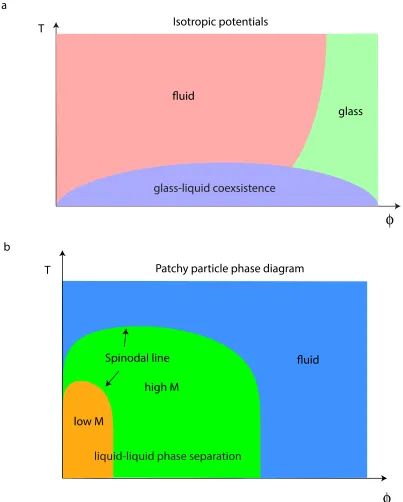
line” at low temperature side. The glass line intersects with the gas-liquid spinodal line for these systems. Therefore, at low temperature, it is not possible to obtain a disordered, homogeneous arrested state; all states will exhibit phase separation. What will the phase diagram be for the anisotropically interacting patchy particle systems?

Bianchi and colleagues [12] approached this question using a Monte Carlo computa-tional modeling method. They studied the phase behaviors of patchy particle systems with different numbers of patches with broad density and temperature ranges. They modeled the interactions between patchy particles by an isotropic repulsive hard sphere interaction and an anisotropic attractive patch interaction. The anisotropic interaction is exerted at cer-tain spots on the particle surface, and the number of these spots per particle is called the coordinate number,M. Their simulation was performed on systems with different average coordinate numbers,<M>.

(27)

0.1 as an unstable non-homogeneous phase. This patchy particle phase diagram has been experimentally verified using the interactions between DNA oligomers as the patches [13, 68, 94]. Given this theoretical understanding, new materials with bizarre phase properties were predicted and discovered, such as reaching a reversible gelled state from a disordered state by heating [95] and the discovery of a gelled, “empty liquid” in a clay [99].

To sum up, more and more study has focused on the patchy particle systems, both experimental and computational/theoretical. This is not only because these patchy parti-cle systems are a rich new theoretical tool for studying the fundamental building blocks of biological systems, but they also show new physics with applicable properties. Novel phase behaviors have been found, and self-assembly of attractive particles with isotropic interactions are studied both for non-biological particles and for proteins.

1.2 Underwater vision

As we have seen above, patchy particle systems can create a huge variety of patterns and structures, and have attracted more and more attention recently. This is particularly ‘hot’ in biological systems, where our understanding has exploded dramatically in past decades. In this dissertation, I will focus on the self-assembly of a specific biological system, squid eye lenses. I will then compare the lens system to a separate but physically similar material, preserved Chinese “century eggs”, or pidan in Chinese. The goal is to understand the self-assembly mechanism, and to propose a theory to explain it. Since the proteins in a squid lens are globular proteins, I will engage patchy particle theory to help understand the construction of the lens.

(28)

1.2.1 Eyes, lenses, and underwater vision

With the sun shining on earth from the beginning of life, life has evolved to capture the image from objects around in order to survive in the living environment. The structure of the image capturing systems vary in a continuum, from photon receptors of a few cells to complex camera-like eyes. In fact, it is not obvious how to define what an eye is, because nearly every imaginable intermediate exists between an eye with high resolution and the simple light sensor. However, the big distinction between an eye and a light-sensitive cell is whether the system is capable of spatial vision [73, 75].

Spatial vision describes a kind of vision which perceives light intensity with spatial distribution. It requires some mechanism to focus incident photons onto a set of photore-ceptors that are overall independent from each other. Given these, a camera-like structure of an eye is a good candidate, and has been found in a lot of species. This eye structure requires a lens to focus light, and the appearance of a lens marks a giant leap in the eye evolution. Nillson and Pelger have studied the course of the evolution of lenses by using computational methods [83]. They showed that an animal might have used 200,000 gen-erations to evolve a pin-hole-like structure from a flat layer of photon sensitive cells. A lens could plausibly have appeared after 38,000 additional generations. After that, the eye and the lens could have modified themselves and reached the configuration similar to a modern eye within 120,000 generations. During this process, the appearance of a lens is crucial because a pin-hole structured eye can only reach a limited vision in an evolutionary dead-end, but a lens can break the bottleneck and form a camera-like eye to achieve better spatial vision.

(29)

receives. This is crucial to underwater animals because the total number of photons in the aquatic environment is low. In fact, the number of photons in water is attenuated roughly by a factor of 10 for every 70 meters [73, 75], while animals have good spatial vision down to abyssal depths. For animals like squid whose habitats are at 300 meters deep, the irradiance is 10,000 times dimmer compared to the land. Thus, underwater animal eyes have adapted to this darker environment by having a bigger lens with a shorter focal length in their eyes.

1.2.2 Spherical lens

To maximize the amount of light reaching the retina, a spherical lens is optimal for camera-like eyes because it is the shape to achieve highest sensitivity. There are two features which determine the sensitivity of an eye: the lens diameter (for underwater eyes) or the pupil size (for terrestrial animals)D, and the solid angleWwhich each receptor covers to accept light. The size of a lens or a pupil behaves like an aperture of a camera and the number of photons getting through is in proportion to the area of the aperture, which is D2. The number of photons that a receptor accepts is also in proportion to W, which is in reverse proportion to the square of the focal length f, as is shown in Figure 1.3. The sensitivity is expressed as

SµD2W. (1.1)

(30)

D

f

Ω

Figure 1.3: Spherical lenses for underwater vision. A spherical lens is required to maximize the photon flux for an underwater eye. Having a spherical lens can increase the aperture and decrease the focal length. Both of these result in an increase of the photo flux. The eye apertureDis the opening that allows photons getting through. The focal length is f, and the solid angle from the center of the lens to the retina is labelled asW.

a ‘lenticular’ shaped as is found in human eyes. This lens design has evolved in parallel in both fishes and squids.

1.2.3 Spherical aberration

(31)

1.2.4 Maxwell’s fish lens equation

The refractive index at different radial positions of a spherical lens can be calculated using geometric optics. The relationship between a refractive index and a lens radius that will correct for spherical aberration can be calculated using the Maxwell’s fish lens equation [23]

n(r) = nc

1+ _ar 2. (1.2)

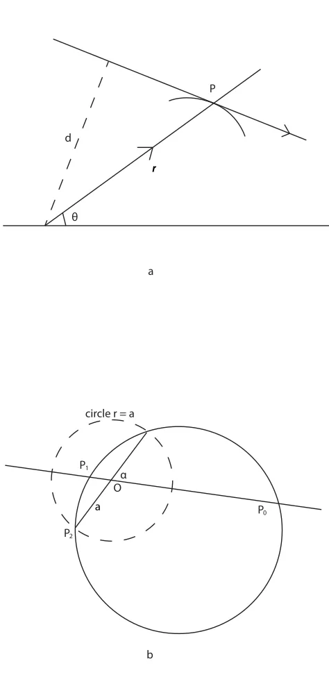
Here,r is the radial position,ncis the refractive index of the core, and ais the radius of a reference sphere (Figure 1.4b). This equation describes a distribution with spherical sym-metry where refractive index increases with decreasingr, and the maximum of refractive index appears at the very center of the lens, with the value ofnc. With this refractive index distribution, a spherical lens can focus light into a point, as is shown in the following: in a medium with spherical symmetry, the equation of a ray path can be written in this form:

q =c

Z r _dr

rpn2₍_r₎_r2 _c2, (1.3)

whereq is azimuthal angle and c is a constant. The details can be found in Figure 1.4a. Plugging in Equation 1.3, we have

r2 _a2

rsin(q a)= r2

0 a2

r0sin(q0 a), (1.4)

whereP0(r0,q0)is a fixed point anda is a constant. The physical meaning of this equation

is shown in Figure 1.4b. For any incident light passing through a pointP1, they will meet

atP0which is at the line joiningP0toOwith , and the paths of the rays are arcs of circles.

Hence, a medium with its refractive index distributed as in Equation 1.2 focuses each point on the spherical surface to the opposite point on the same surface.

(32)

θ

P

d

P

O

P0

P2

circle r = a

1

α

a

b

r

a

Figure 1.4: A refractive index gradient can eliminate spherical aberration in a spherical lens. The ray path of in a medium with spherical symmetry is shown in (a). The position of any pointPin the ray path is described as the vectorrand the azimuthal angleq. Figure (b) shows that a Maxwell’s fish lens can focus light into a point, whereP0(r0,q0)is a fixed

(33)

index is described in the Maxwell’s fish lens equation. This equation requires that the refractive index increases monotonically from the periphery to the core of the lens.

1.3 Vertebrate eye lens

All vertebrate lenses which have acute vision are graded refractive index lenses. The shape of an underwater vertebrate eye lens is a sphere. In the development of a vertebrate lens, they are generated from ectodermal cells. The mitotically active cells are located only in the outer epithelial monolayer around the lens [90]. There is a region in the epithelium where cells elongate into fiber-like structures. After the elongation starts, nuclei and mito-chondria are ejected from the lens fibers. Therefore, only cells in the epithelial monolayer can duplicate and create lens proteins. The cells are laid down in layers after the elongation from the epithelium at the periphery of the lens. Throughout the growth of the lens, these cells are displaced toward the center. The resulting structure of the lens has distinct layers of cells which are maintained in the mature organ. The lens grows throughout the whole animal’s life, but the rate of the lens growth is only rapid in the embryonic development and in early life after birth [90].

1.3.1 Vertebrate lens protein

(34)

crystallins are evolutionarily related to stress proteins [5]. There is also a 35 kDa crystallin found in a frog lens [119].

a-crystallins are related to small heat-shock protein family [56] and are also expressed in heart, skin, brain, retina and other tissues. They are polydisperse oligomers with the molecular weight between 800 to 900 kDa, containing more than 40 subunits. There are two a-crystallin genes, aA and aB, sharing around 60% sequence identity [16]. a A-crystallin is expressed only in the lens [108] and aB-crystallin is stress-inducible. The interactions between a-crystallins are repulsive in a physiological solution [116]. The in-teractions involve hard-core and screened Coulomb inin-teractions, which are responsible for lens transparency [25, 46].a-crystallins are essential to keep transparency of the vertebrate lens, given that they are presumed to be function both as structural proteins and as protein chaperones [17].

b-crystallins also form oligomers, and monomers range from 22 to 28 kDa in

molecu-lar weight. g-crystallins are mostly monomers, with molecular weight about 21 kDa. The main difference betweenb- andg- crystallins in sequence is that compared tog-crystallins,

b-crystallins have N-terminal extensions. The basicb-crystallins have C-terminal exten-sions as well [8, 53, 65]. The interactions between b-crystallins are repulsive, and the interactions betweeng-crystallins are attractive [116].

1.3.2 Transparency of vertebrate lens

Lens transparency in vertebrates is achieved by complex interactions and assembly of the constituent proteins. Physically, transparency requires that the protein density fluctuation is maintained low at the length scales of visible light wavelengths. There are two major ways by which a cataract happens in a vertebrate lens: protein unfolding and phase separation.

(35)

has been found to act as a chaperone [90]. Experimental results show that a-crystallins suppress thermally-induced aggregation of various enzymes, includingb- andg- crystallins [56]. However, a cataract may still happen when an immature lens fibre cell is overwhelmed by stress if there is misfolding of a mutant crystallin, or when a mature lens fibre cell uses up the chaperone capacity ofa-crystallins [90].

Another kind of cataract, however, happens without protein misfolding. It is caused by changes in solubility or attractive properties in lens proteins, which leads to a phase separation [90]. Due to this liquid-liquid phase separation, big density fluctuations result in scattering of light. For a mixture with attractive interactions between particles at low temperature and low concentration, the mixture is separated into two phases at mesoscopic scale with different solute concentrations. This separation can be droplets of a liquid phase of the solution component suspending inside another liquid phase of the same solution com-ponent [20, 79], or even sediment to the bottom of the container. These two liquid phases have different refractive index, and scattering comes from the interface of these two phases. With millions of interfaces between the two phases acting as little scatterers, opacity oc-curs. Concentratedg-crystallins, which have van der Waals and other attractive forces, have been observed with liquid-liquid phase separation [70]. This is why lowering temperature of a bovine lens results in droplet-like liquid-liquid phase separation, and opacity in the lens, a so-called “cold cataract” [79]. For an underwater lens, turbidity is more likely in the periphery, where the protein packing fraction is similarly low [9, 79, 114]. A little protein aggregation can result in strong density fluctuations. In the core of an underwater lens, the ultradense gelled condition suppresses of the density fluctuation, reducing the unwanted light scattering [79].

(36)

with the increase ofa-crystallin concentration in the solution [124], indicating a repulsive interaction between thea-crystallins. But this repulsion is weak, and with the combination of this repulsion and depletion, a short-range liquid-like order forms fora-crystallins. The predicted quaternary structure of these proteins displays tetrahedral symmetry [124]. Since the molecular weight ofa-crystallins can be large, this short-range ordered size is close to visible light and this is how a vertebrate lens keeps transparency.

The short-range order disappears at the core of a vertebrate lens. No peaks have been seen in SAXS experiment at the core of either a bovine or a fish lens. This disappearance is achieved by the increase of polydispersity in the sizes of the crystallins and the increase in concentration of the smallg-crystallins which occupy the void space [79].

1.4 Squid eye lens

The material evolutionary story for a squid lens is quite different from a fish lens. The lenses of cephalopod eyes are composed of independently developing anterior and posterior hemispheres that later fuse to become the mature, spherical lens. These hemispheres dif-ferentiate from an overlying layer of ectodermal cells [117]. Both segments are developed from separate groups of ectodermal cells referred to as lentigenic cells [126]. S-crystallins accumulate first in the posterior segment and protein synthesis begins in the anterior seg-ment two days later. The cephalopod lens continues to grow throughout maturity, and S-crystallins are made throughout the squid’s life [126]. However, as in the vertebrate lens, mature lens cells lack nuclei and mitochondria; there can be no protein turnover after a lens cell matures and is laminated onto the existing spherical lens structure.

(37)

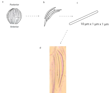
In fact, when we look at the lens under microscope, a lens cell has to be isolated from the others to have enough refractive index difference with the environment for us to observe it, as is shown in Figure 1.5d. The lens structural proteins are contained inside these cells.

10 μm x 1 μm x 1 μm

a _b _c

d Posterior

Figure 1.5: Cellular structure of a lens. The lens is composed of cells which are laid down parallel to each other on a path from the zenith to the nadir of the sphere. The lens has a membrane which separates the lens into the posterior and anterior halves (a). The cells have filament-like shape next to each other (b,c). The cell image under an optical microscope is shown in (d).

1.4.1 Squid lens protein

(38)

soluble proteins [19]. There are dozens of different S-crystallin forms expressed in a single lens that are 46-99% identical to each other by amino acid sequence [123]. S-crystallins are evolutionarily derived from glutathione S-transferase (GSQ), a liver detoxification enzyme, which may also play a role in molecular chaperoning, similar toaA crystallin in vertebrates [64]. For S-crystallins, all the isoforms except lops4 (Figure 1.6b) have a few inserted peptides with various lengths in the sequence of GSQ [117, 123]. These exons correspond to a disordered, loop-like structure protruding from the folded surface of an S-crystallin. The presence of the loop is correlated with a loss of GSQ enzymatic activity in a given protein [117]. A single S-crystallin is a dimeric structure, with each monomer containing a mixture ofb anda structure in the N-terminal domain, and alla-helix in the C-terminal domain. Comparing the octopus S-crystallins to the squid S-crystallins shows that most of the members of this lens protein family in squids expanded after the divergence of these two taxa 200-300 mya [117, 120], and the major S-crystallins seem to have undergone positive evolutionary selection correlated with a lens structural role [120].

The proteins were cataloged by Sweeney and colleagues into two groups based on the loop length: long-loop proteins (molecular weight⇡27 kDa) and short-loop proteins (⇡25 kDa), as is shown in Figure 1.6. They used homology modeling to calculate the surface charge of these S-crystallin isoforms [114]. They found that the long-loop proteins have higher net charge (+4.8) compared to the short-loop proteins (+2.8).

(39)

a

b c

5 nm

Figure 1.6: S-crystallins and glutathione S-transferase (1GSQ). The protein structure of 1GSQ (a), a short-loop S-crystallin (b), and a long-loop S-crystallin (c) are shown. The protein structure 1GSQ is from the liver-expressed enzyme related to the lens-expressed S-crystallins. The short-loop S-crystallin and long-loop S-crystallins expressed in the lens differ in loop length. Lops4 is shown here as an example of short-loop S-crystallin (b).

are more recently diverged from the rest of the family compared to the short-loop proteins. These highly-charged long-loop proteins are under more-intense positive selection, and their appearance is approximately simultaneous with the appearance of the complex GRIN lens. These results suggest that long-loop proteins are crucial to form the GRIN lens.

(40)

surface charge

6

8

10

8

10

12

10

8

14

8

6

4

6

8

3

long-loop proteins

short-loop proteins

higher surface charge

low surface charge

(41)

evolved independently from vertebrate lenses. All of the above suggest that there is an-other mechanism of how a squid lens builds a gradient index and maintains transparency.

1.4.2 Previous hypothesis for lens transparency

To study the possible mechanism of how a squid lens builds and maintains graded index and transparency, Sweeney and colleagues studied the S-crystallin distribution in the lens with respect to the lens’s optical properties [114]. They found that the long-loop proteins are expressed more in the peripheral, low-index regions of the lens. At the core of the lens, it is mostly composed of short-loop proteins. Further, they found that long-loop proteins are highly charged, with much higher positive surface charge compared to short-loop proteins. Therefore, they hypothesized that the mechanism for a squid lens to keep transparent in the periphery of the lens is to have proteins here highly charged, and the repulsive screened coulomb interaction between these proteins prevents them from aggregating. Then short range order forms in this mechanism, similar to the repulsive mechanism for transparency of vertebrate lenses, and no aggregations or accumulations are allowed by the screened Coulomb repulsion. This hypothesis also predicts that there is no larger structure formed at length-scales larger than a few protein diameters, and proteins will be homogeneously distributed. In this hypothesis, thermal fluctuations are reduced by a repulsive jamming in the system, and proteins in the periphery form a repulsive glass. In the core of a squid lens, they predicted that since the protein density is so high, the space is all packed with proteins, so there is little density fluctuation in the core of the lens. The increase in concentration of short-loop proteins in the center would be due to the requirement of high packing frac-tion — smaller proteins without long-loops can be packed denser compared to long-loop proteins. The core of the lens is also jammed, required by the high protein density.

(42)

lens is a jammed system, with charge-charge repulsion between jammed proteins in the periphery of the lens, and close-packing interactions in the core.

In this thesis, I will conduct experiments to investigate in our previous hypothesis. I will check whether the old hypothesis is consistent with my experimental results. If not, what is the mechanism that the proteins assemble in the squid lens to achieve the GRIN lens with such a largef span? Are the proteins in the lens patchy particles? What is the phase of the lens system? Can the phase diagram provide us with a solution to the assembly of the lens system? Further, are there any other protein systems that are similar to the squid lens system with proteins as the patchy particle? My research will focus on these questions.

1.5 Outline of this work

(43)

Chapter

2

Proteins in the squid lens

(44)

consis-tent with my homology models, and are well-folded in the lens. At the end of this chapter, I studied the surface charge of the protein by conducting isoelectric focusing experiments (IEF). All of these properties from the lens proteins will be essential to construct my hy-pothesis to explain the lens as a self-assembling system of graded refractive index in the subsequent two chapters.

2.1 Introduction - protein identification

Squid lens cells are essentially membranous bags of S-crystallin proteins which are lami-nated together and organized into a sphere. The major protein components in a squid lens are S-crystallins, as was mentioned in Chapter 1. To understand the lens system, I need to know what isoforms of S-crystallins are contained in the lens, and where they are expressed. The exact protein composition ofLoligolenses was studied using Illumina technology RNA sequencing by my labmate Tom Dodson. The sequencing assembly results showed a total number of 53 unique S-crystallins expressed in the lens, 14 of which were assembled as full-length constructs. These proteins are very similar to S-crystallin sequences currently in genbank from other species, and thus, we identify them as S-crystallins. The major dif-ferences between the proteins in our dataset appear mainly in the region of the sequences that encode a loop-like structure in the center of the two folding sub-domains of the con-served enzyme. In fact, we identified 39 unique “loop” sequences of variable length, and in all cases they are predicted to encode an unstructured, soluble loop protruding from the folded core of the homodimeric protein. This loop accounts for the observed differences in molecular weight between S-crystallin isoforms.

(45)

2.2 Sample collection and lens layers

Loligo forbesii squid lens tissue was obtained from the Marine Biological Laboratory

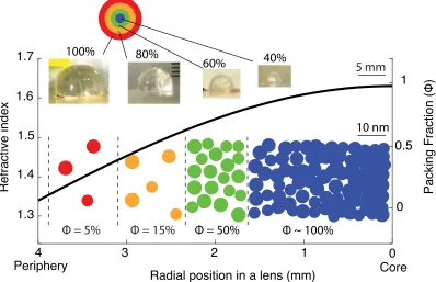
at Woods Hole, MA, and coastal campus of University of Connecticut at Avery Point. Sthenotuethislens tissue was obtained with squid jigs from the R/V Kilo Moana from var-ious sites in offshore Hawaii. Lenses were excised from the suspending tissue, and fixed immediately for TEM, or stored at -80 C either alone or in RNA Later (Life Technologies #AM7020, Grand Island, NY 14072) for use in other experiments. Lenses were thawed on ice and divided into anterior and posterior hemispheres along the naturally-occurring membrane separating the two. For most of our experiment, the posterior hemispheres were dissected into four concentric hemispherical layers, shown in Figure 2.1. The thickness of each layer is somewhat arbitrary and varies with different lens samples. Therefore, these dissections were digitally photographed to make a record of the radial position of each tis-sue subsample. On average, the peripheral layer usually ranges from 80% to 100% of the total lens radius, and we call it the 100% layer; the next layer, the 80% layer, ranges from 60% to 80%; the 60% layer ranges from 40% to 60%, and the radius of the core sample is typically less than 40% of the total radius of the lens.

2.3 Refractive index matching experiment

The squid lens is interesting because a graded refractive index sphere is required to have acute vision underwater (see Chapter 1). To start, we experimentally studied the refractive index at different positions in a squid lens and fit these data to theoretical expectations about refractive index distribution. We did several independent experiments and confirmed that Loligolenses have the expected density and refractive index distribution with radius that is described to first order by the Maxwell’s fish lens equation.

(46)

10 nm

Φ = 5% Φ = 15% Φ = 50% Φ ~ 100%

4 3 2 1 0

1.3 1.4 1.5 1.6 1.7

Radial position in a lens (mm)

Refractive index

100% _80%

60% 40% _{5 mm}

0 0.5

1

Core Periphery

Figure 2.1: Dissection of the lens, refractive index, and packing fraction distribution. Hemispheres of lens tissue were dissected into four concentric layers labelled as 100%, 80%, 60%, and 40% layers (shown in the images); the exact thickness of each layer varies with different lens samples. The relationships between refractive index, protein packing fraction and lens radius are plotted in the black curve. This relation is obtained by fitting the Maxwell’s fish lens relation using my index oil matching result, as explained in the text. Colored circles show the approximate protein density required at each position to generate the required refractive index gradient.

spherical aberration (Chapter 1). Using geometric optics, the refractive index at different radial positions of a ratio lens can be calculated using the Maxwell’s fish lens equation:

n(r) = nc

1+ _ar 2 , (2.1)

(47)

labs, Cedar grove, NJ). Immediately after immersion, we photographed each layer in index-matching oil, and using these photographs, we recorded the radial position of the tissue sample that was invisible in each of the two index-standard fluids. With this information about exact refractive index at two radial positions, we can estimate the refractive index at all radial positions in the lens with the Maxwell’s fish lens equation (Eq. 2.1).

The result of the index matching experiment shows that for a single example lens, tissue samples from approximatelyr=3 mm radial position disappear in then=1.45 standard, and samples from r =1.9 mm disappear in the n = 1.55 standard. Using equation (1), we havenc =1.63 and a=8.6 mm, and the predicted refractive index at different radial position of the lens is

n(r) = 1.63

1+ ₈r_.₆ 2 . (2.2)

The distribution of the refractive index is shown in Figure 2.1. From this equation, the inferred refractive index at the outer most radial point in the lens is then 1.37, close to that of seawater withn=1.34. In the core of the lens, the inferred refractive index is 1.63. See Table 2.1 for the refractive index at other positions in the lens.

2.4 Protein concentration in the lens

(48)

2.4.1 The gradient of refractive index is achieved by a gradient in the

protein concentration

To check whether the refractive index gradient was achieved by having a graded protein concentration, I calculated the refractive indicesnpof the dry proteins in the lens using the Lorentz-Lorenz formula

n(p) = s

2Rp+v¯p ¯

vp Rp , (2.3)

where Rp is the refraction per gram of the protein, and ¯vp is the protein partial specific volume, which is the weighted average of the partial specific volume of each amino acid [74]. I calculatedRp for all the proteins in the lens based on the amino acid sequences in our sequencing data. These proteins have been studied before [114] evolutionarily, and our previous study presents the evolutionary tree of these proteins. From there, I can estimate the refractive increment, or increase in refractive index with increase in protein concentra-tion (c) at 578 nm, using the Wiener equaconcentra-tion [135]:

dn dc =

3 2v¯pn0

n2_p n2₀ n2

p+2n20

. (2.4)

In this equation, n0 is the refractive index of the medium, which was set to be 1.334. I

calculated refractive index incrementdn/dcfor all the proteins in the lens, and compared thedn/dcfor the new emerged proteins and the old proteins. Then I used Zhao’s method [135] to calculate the predicteddn/dcas the increment of protein concentration.

(49)

are no major differences in refractive increment among proteins in the squid lens, and therefore no evidence that squid lenses increase refractive increment in the center of the lens by changing the amino acid composition of the crystallin proteins, as was shown by Zhaoet alfor vertebrates [135].

In short, the refractive index gradient in a squid lens is achieved by having a gradient in the protein concentration. I now want to estimate the predicted protein concentration. Given that we havedn/dcof the protein assembly and the refractive index distribution, we need to have one data point with both known refractive index and known concentration to estimate the whole concentration distribution in the lens. I measured both these properties at the core of the lens, where the protein concentration is the highest across the lens.

2.4.2 Core of the lens, measurement and theoretical estimation

To find the protein concentration in the lens core, I measured its density by comparing it to fluids of known density. I did this by submerging additional samples from the very core of the lens in potassium iodide solutions of known density; a tissue sample will float in less-dense fluids, and will sink in more-dense fluids. I can also infer the refractive index of the core from the Maxwell’s fish lens equation. As reported below, these two methods of estimating the core refractive index were in good agreement.

(50)

extrapolating from direct index measurements using Maxwell’s fish lens equation. The fact that the inferred core refractive index is the same as dry lens protein is another piece of evidence which indicates that there is no water in the core of the lens.

To sum up, our density experiment at the core of the lens shows that the core almost entirely composed of proteins with little water in it. This is required to achieve the high refractive index. This conclusion is further supported by our small angle x-ray scattering (SAXS) result as will be discussed in Chapter 3. Next, I will estimate the protein concen-tration at different radial positions in the lens.

2.4.3 Predicted protein concentration of a squid lens at different

ra-dial positions

The concentration and the packing fractionf of the protein in the lens at all positions can be estimated: Given a radial position in the lens, the refractive index was calculated using the Maxwell’s fish lens equation. The required protein concentration can be calculated using the refractive index increase increment equation 2.4.

Given both the core density and dn/dc, the calculated protein packing fraction at dif-ferent radial positions of the lens is:

f =0.75c= 6.1

1+ (r/8.6)2 5.1. (2.5)

The result is shown in Table 2.1 at several radial positions of the lens, with the bold refrac-tive indices the measured data. The packing fraction of protein in lens tissue spans from

⇠5% in the periphery to 100% in the core of the lens. This result is also shown in Figure 2.1.

(51)

Radius(mm) RI Packing Fraction 3.7 1.37 0.04 3.0 1.45 0.33 1.9 1.55 0.71 1.3 1.59 0.86 1.0 1.60 0.92 0 (inferred) 1.63 1.0

Table 2.1: Refractive indices at different radial positions in a squid lens. The radial position of a lens, refractive index (RI), and the packing fraction are listed. The bold numbers in RI are obtained directly from the index oil matching experiment, and the rest are calculated.

concentrated than the periphery of the lens. Throughout this span of protein concentration, transparency is required at all positions in the lens. The question is how does the lens maintain a low protein density fluctuation at such a large protein concentration span? How does the lens avoid liquid-liquid phase separation throughout the lens, especially in the periphery where protein concentration is low? To approach the answer, we need to know the distribution of S-crystallin isoforms at different positions in the lens.

2.5 Relative protein abundance distribution

(52)

2.5.1 Relative protein abundance at different radial positions in the

lens

Polyacrylamide gel electrophoresis (SDS-PAGE) separates the proteins by their molecular weight. Proteins unfolded by SDS are loaded into a gel, and an electric field is applied to the gel. Proteins with higher molecular weight will migrate slower in the gel compared to the smaller proteins.

In this experiment, lenses were dissected into four concentric layers and stored in RNA later at -80 C. Then the subsamples were homogenized with plastic micropestles in 1.5 ml microcentrifuge tubes in XT sample buffer (Bio-Rad Laboratories, Hercules, CA, #161-0791) with XT reducing agent (Bio-Rad 161-0792) and protease inhibitor cocktail (#P8849-5ml, Sigma Aldrich, St. Louis, MO) added according to the manufacturer’s in-structions . These samples were heated to 95 C for 5 minutes to denature the constituent proteins. Then the solution was centrifuged at 14,000 rcp for 1 minute to remove any re-maining solids. This procedure resulted in no visible pellet, suggesting that lens proteins were entirely solubilized. I used a BioRad 10% precast polyacrylamide 12+2 well gel (Bio-Rad #345-0111), with XT MOPS running buffer (Bio-(Bio-Rad #161-0788) for electrophoresis. The gels were stained with Invitrogen SafeStain according to manufacturer’s instructions (Life Technologies, #LC6060). Then the gels were scanned in transparency mode on a desktop scanner (HP Scanjet G4050). I calibrated both the quantities of protein loaded in the gel, and the images from the scanner such that the resulting grayscale intensities of pro-tein bands in the scanned images were linearly proportional to the concentration of propro-tein in the band.

(53)

of the molecular weights of the proteins in the standard. The gaps between protein bands were treated as the intensity baseline and were corrected by the built-in MATLAB function ‘msbackadj’. The greyscale intensities of the samples were then normalized relative to total S-crystallin protein content by dividing by the sum of all values in the range of 20 to 40 kDa for a single sample.

At all radial positions, greater than 90% of the protein in the lens was found in two overlapping, broad bands migrating on the gel. These broad bands represent two major molecular weight classes of S-crystallin, one with majority molecular weight at around 24.5 kDa and the other with majority molecular weight around 26.5 kDa, as is shown in Figure 2.2. It was not possible to completely separate these two bands, which are the com-posite migrations of many S-crystallin isoforms, and seem to represent the mean migra-tion posimigra-tion of the long-loop and short-loop categories of S-crystallin proteins. Therefore, based on information from our RNA sequence data, I chose to define the boundary between the 24.5 kDa (short-loop) and 26.5 kDa (long-loop) protein migration bands to be 25 kDa. The ratio between 26.5 kDa band to 24.5 kDa band decreases significantly from 1.0 in the periphery of the lens to 0.06 in the core, shown in Figure 2.2. There are also two minor bands in each sample, at 32 and 36 kDa, similar to proteins in a frog lens [119]. The very high molecular weight S-crystallins (⇠36 kDa) behave differently from the 26.5 kDa and 24.5 kDa molecular weight S-crystallins. They are at a minimum in the periphery of the lens, and increase in abundance with decreasing lens radius to a maximum of 7% of total protein at a lens radius of 2 mm. The abundance of these proteins then decreases again to a prevalence of 1% to 3% in the lens core.

(54)

0 9 27 46 64 83 101 120

24 26 28 30 32 34 36 38

molecular weight (kD)

loop length (#aa’s)

Conc en tr ation (a.u .) radius(mm)

long / short

0.5 (core) 1 1.5 2 2.5 3 3.5 0 0.2 0.4 0.6 0.8 1 1.2 a b 25 kDa 20 kDa 37 kDa 50 kDa 100% 80% 60% 40% layer 0 1 0.5

(55)

clue on how the lens assembles, as will be discussed at the end of this section and chapter 4. For now, I further investigate the protein composition by comparing the RNA sequencing result to the SDS-PAGE result.

2.5.2 Peak decomposition

(56)

20 22 24 26 28 30 32 34 36 38 40 0

0.5 1

Molecular weight (kDa)

Concentration (a.u.)

20 22 24 26 28 30 32 34 36 38 40

0 0.5 1

20 22 24 26 28 30 32 34 36 38 40

0 0.5 1

20 22 24 26 28 30 32 34 36 38 40

0 0.5 1

23.7

24.525.025.726.5 kDa

Molecular weight (kDa)

Concentration (a.u.)

(57)

The result showed that although similar-looking broad peaks are present at all lens radii, S-crystallin isoforms in each major broad composite peak continuously shift to a larger molecular weight as a function of lens radius (Figure 2.3). Though the exact position of the sub-peaks vary at different radial positions in the lens, the wide composite peaks centered at 24.5 and 26.5 kDa are mainly comprised of S-crystallins with molecular weight 23.7, 24.5, 25.0, 25.7, and 26.5 kDa.

The close fitting of SDS-PAGE data to transcripts found in RNA sequencing, along with previous published data about squid lens composition [114] suggests that the lens is composed of many variations of a single glutathione s-transferase-related protein fold. The most salient difference between these closely related proteins is the length and composition of a loop inserted between the two folding domains of the protein. There is a clear increase of the relative abundance of the low molecular weight S-crystallin isoforms from the pe-riphery to the core of the lens. The lowest two major sub-peaks in molecular weight are comprised of S-crystallins with molecular weight 24.5 and 25.1 kDa in the periphery of the lens, whereas in the core, it is comprised of 23.7 and 24.35 kDa. This shift shows a clear trend of decreasing average molecular weight from the periphery to the core of the lens. At the high molecular weight side, the 26.5 kDa sub-peak component comprises 22% of the total S-crystallin composition in the periphery, and this proportion decreases to 6% in the core. This trend also appears in the 25.7 kDa sub-peak. The percentage of this isoform drops from 9% to 2% from periphery to the core of the lens.

(58)

I used the protein structure estimation technique called homology modeling to estimate the atomic-scale protein structure of the ensemble of S-crystallins.

2.6 Homology modeling of the proteins in the lens

Homology modeling provides a method to estimate atomic structure and therefore the sur-face characteristics of the different S-crystallin isoforms, as well as a plausible initial con-formation of the apparently unstructured cytoplasmic loops.

To estimate the structure of S-crystallin isoforms, I used homology modeling which constructs the protein secondary and tertiary structure based on homologous, known pro-tein structures. Specifically, S-crystallins tertiary and quaternary structure were estimated using the Swiss-model (http://swissmodel.expasy.org/). The predicted S-crystallin models were built based on homo-oligomeric structures from selected proteins from the SWISS-MODEL template library. Glutathione S-transferase (1GSQ) was the main known protein structure selected as the template for all of the isoforms of S-crystallins. 1GSQ is the progenitor of the squid lens S-crystallin [61, 123]. It has a dimeric structure. The squid S-crystallin have a few inserted peptides with various lengths in the sequence of 1GSQ. The similarities between 1GSQ and S-crystallin are the reason why 1GSQ are chosen to be the homology model template.

(59)

Increase amino acid number in the loop

50 Å

(60)

loop proteins with 103 and 106 amino acids, there are no templates which are similar in the loop amino acid components. As a result, homology model fails to output a predicted structure for them. If the 106 amino acid loop is extended and unfolded in the solvent like the other shorter loops appear to be, it can easily extend to 300 ˚A away from the folded body of the protein. In general, basic residues tend to be exposed on the surface of the pro-tein, while the disordered loop inserted in the otherwise conserved 1GSQ sequence tends to take a flexible, unfolded configuration in the solvent.

2.7 Circular dichroism spectroscopy

(61)

temperature was controlled by a Peltier heating and cooling system. The analysis of the CD spectrum is performed using the online server CAPITO [129].

The absorbance difference between the two oppositely circularly polarized light sources at different wavelengths is shown in Figure 2.5. Two minima were observed in the ab-sorbance at 213 nm and 223 nm. A maximum was located in the middle of these two minima. The two minima are consistent with a helix structure [28]. This fact is consis-tent with our homology modeling that the S-crystallins are mostly composed of helical structures.

The spectra values at 200 nm and 222 nm are plotted to estimate the folding properties of the lens protein together with these values from known folded and unfolded proteins, shown in Figure 2.5. The lens protein locates in the middle of the globular proteins. This is consistent with the fact that S-crystallins are globular proteins. The lens protein does not locate among the unfolded proteins. Therefore, the circular dichroism experiment shows that the proteins in the lens are well folded.

2.8 Isoelectric focusing (IEF)

(62)

Lens

Figure 2.5: Circular dichroism spectroscopy of lens protein. The circular dichroism ab-sorbance (Q) from a ground lens tissue with buffer subtracted in shown in the top figure. There are two valleys at 209 and 222 nm, and a peak at 192 nm. These features are consis-tent with alpha-helical structure. The bottom figure shows the absorbance at 200 nm and 222 nm of the lens protein compared to known proteins in their native form and unfolded form using the online server CAPITO [129]. The lens protein locates in the middle of the globular proteins, which is consistent with the structure of S-crystallin. This indicates that the proteins in the lens are well folded.

(63)

in 30% methanol and 12% trichloroacetic acid, then stained with silver stain (Bio-Rad Sil-ver Stain Plus Kit #161-0049). The gel results reported here show the data from the first gel for isoelectric point PI <6 and data from the second, switched electrode gel for PI >6. The isoelectric point of the 36 kDa S-crystallins are calculated using the online server ExPASy from the amino acid composition [14, 15, 50].

4

5

6

7

8

9

10 Isoelectric point

Protein abundance (a.u.)

Figure 2.6: IEF-PAGE of lens proteins. Lens proteins are separated by their isoelectric point (PI), and the abundance of each PI is shown in the figure. Curves are colored accord-ing to the radial position in the lens the samples were taken from, with red 100%, orange 80%, green 60%, and blue 40%. The sharp peak at isoelectric point of 5.4 is very likely from the 32 and 36 kDa S-crytallin isoforms. The peaks atPI_⇡8 may come from the long-and short- loop S-crystallins.

(64)

peak at PI⇡8 for all layers in the lens. I attribute this broad composite peak to the mixture of S-crystallins with molecular weights from 23 to 28 kDa. This spectrum of peaks is consistent with our SDS-PAGE result that the proteins in the lens are a mixture of dozens of S-crystallin isoforms, rather than a binary mixture of two proteins. The acidic part from the IEF-PAGE shows a sharp peak at PI=5.4 for all layers. This peak is associated with the S-crystallins with super long loops at 36 kDa. The calculated PI is 5.2 for these proteins because the loops of these proteins are highly negatively charged. This result is also consistent with our SDS PAGE result that there are 36 kDa S-crystallins at all positions in the lens.

In short, this IEF-PAGE result shows that majority of S-crystallins are positively charged at all positions in the lens. There is a wide distribution of protein PIs, ranging from 5 to 9.5. This is consistent with our SDS-PAGE result in that the lens is composed of a mixture of dozens of S-crystallins. The super long loop protein with molecular weight 36 kDa is negatively charged because the long loop contains more negatively charged amino acids. Across the different positions in the lens, there is not much difference in the PI of the protein composition.

If the charge of the proteins are high enough and the phase of the protein assembly in the lens is repulsive glass, one would expected to see individual proteins in their native form. This will be addressed in the next section.

Superior to one of Glass: Natural Gradient index Lenses via Patchy Particle Self-Assembly

University of Pennsylvania

ScholarlyCommons

Superior to one of Glass: Natural Gradient index

Lenses via Patchy Particle Self-Assembly

Jing Cai

Superior to one of Glass: Natural Gradient index Lenses via Patchy Particle

Self-Assembly

Table of Contents

List of Tables

List of Figures

Chapter

1

Introduction

1.1 Self-assembly

1.1.1 Patchy particle system

1.1.2 Proteins as patchy particles

1.1.3 Phase behavior of a patchy particle system

1.2 Underwater vision

1.2.1 Eyes, lenses, and underwater vision

1.2.2 Spherical lens

1.2.3 Spherical aberration

1.2.4 Maxwell’s fish lens equation

1.3 Vertebrate eye lens

1.3.1 Vertebrate lens protein

1.3.2 Transparency of vertebrate lens

1.4 Squid eye lens

1.4.1 Squid lens protein

long-loop proteins

short-loop proteins

higher surface charge

low surface charge

1.4.2 Previous hypothesis for lens transparency

1.5 Outline of this work

Chapter

2

Proteins in the squid lens

2.1 Introduction - protein identification

2.2 Sample collection and lens layers

2.3 Refractive index matching experiment

2.4 Protein concentration in the lens

2.4.1 The gradient of refractive index is achieved by a gradient in the

protein concentration

2.4.2 Core of the lens, measurement and theoretical estimation

2.4.3 Predicted protein concentration of a squid lens at different

ra-dial positions

2.5 Relative protein abundance distribution

2.5.1 Relative protein abundance at different radial positions in the

lens

2.5.2 Peak decomposition

2.6 Homology modeling of the proteins in the lens

2.7 Circular dichroism spectroscopy

2.8 Isoelectric focusing (IEF)

4

5

6

7

8

9

10

Isoelectric point

Protein abundance (a.u.)

2.9 Native PAGE