University of Pennsylvania
ScholarlyCommons
Publicly Accessible Penn Dissertations
1-1-2013
Arithmetic Constructions Of Binary Self-Dual
Codes
Ying Zhang
University of Pennsylvania, [email protected]
Follow this and additional works at:http://repository.upenn.edu/edissertations Part of theMathematics Commons
This paper is posted at ScholarlyCommons.http://repository.upenn.edu/edissertations/824
For more information, please [email protected]. Recommended Citation
Zhang, Ying, "Arithmetic Constructions Of Binary Self-Dual Codes" (2013).Publicly Accessible Penn Dissertations. 824.
Arithmetic Constructions Of Binary Self-Dual Codes
Abstract
The goal of this thesis is to explore the interplay between binary self-dual codes and the \'etale cohomology of arithmetic schemes. Three constructions of binary self-dual codes with arithmetic origins are proposed and compared: Construction $\Q$, Construction G and the Equivariant Construction. In this thesis, we prove that up to equivalence, all binary self-dual codes of length at least $4$ can be obtained in Construction $\Q$. This inspires a purely combinatorial, non-recursive construction of binary self-dual codes, about which some interesting statistical questions are asked. Concrete examples of each of the three constructions are provided. The search for binary self-dual codes also leads to inspections of the cohomology ``ring" structure of the \'etale sheaf $\mu_2$ on an arithmetic scheme where $2$ is invertible. We study this ring structure of an elliptic curve over a $p$-adic local field, using a technique that is developed in the Equivariant Construction.
Degree Type
Dissertation
Degree Name
Doctor of Philosophy (PhD)
Graduate Group
Mathematics
First Advisor
Ted Chinburg
Keywords
Binary self-dual code, Etale cohomology
Subject Categories
ARITHMETIC CONSTRUCTIONS OF BINARY SELF-DUAL CODES
Ying Zhang
A DISSERTATION
in
Mathematics
Presented to the Faculties of the University of Pennsylvania
in
Partial Fulfillment of the Requirements for the
Degree of Doctor of Philosophy
2013
Supervisor of Dissertation
Ted Chinburg, Professor of Mathematics
Graduate Group Chairperson
David Harbater, Professor of Mathematics
Dissertation Committee
Florian Pop, Professor of Mathematics
Ted Chinburg, Professor of Mathematics
ARITHMETIC CONSTRUCTIONS OF BINARY SELF-DUAL CODES
c
COPYRIGHT
2013
Ying Zhang
This work is licensed under the
Creative Commons Attribution
NonCommercial-ShareAlike 3.0
License
To view a copy of this license, visit
Acknowledgments
I would like to express my sincere thanks to my supervisor Ted Chinburg for his
constant support and guidance throughout my graduate studies. His expertise and
advice are invaluable to me in many ways beyond I could imagine. Among many
other things, I have learned my first class in algebraic number theory from him,
prepared for my qualify exam under his directions, and have had his motivating
collaboration in my first publication. It has been a great pleasure to work with
him. Without his helpful suggestions and instructions, this work would not have
been possible.
I would also like to thank Florian Pop and David Harbater for their constant
help and illuminating discussions in mathematics. Henry Towsner, for serving on
my thesis committee. David Zywina, Jonathan Block and Tony Pantev from whom
I have benefited a lot from their classes. Robin Pemantle and Dennis DeTurck for
giving me many helpful suggestions. Janet Burns, Monica Pallanti, Paula
Scarbor-ough for their constant help in my daily life at the Math department, it is their
I want to express my gratitude to Wenxuan Lu, whose passion for mathematics
has always been encouraging to me. I have enjoyed my life as a graduate student at
Penn to live in a big family of many helpful fellow graduate students: Zhentao Lu,
Adam Topaz, Ryan Eberhart, Taisong Jing, Shanshan Ding, Hilaf Hasson, Justin
Curry, Ryan Manion, Elaine So, Yang Liu, Ying Zhao, Zhaoting Wei, Tong Li,
Haomin Wen, Xiaoxian Liu, Yiqing Cai and many others. I can not forget the
many mornings, afternoons and evenings we spent in DRL discussing problems. I
am also grateful for my friends in Philadelphia: Hao Sun, Yubin Bai, Zhaoxia Qian,
Na Zhang, Rong Shen, Lai Jiang, Yang Jiao, Yin Xia, Chi Liu, Yan Wang, Naibo
Chen, Yuyuan Liu, Shaohui Wang, Zuolu Liu. I am grateful for the many happy
moments they brought in my life.
Last but not least, I want to thank my parents Yongzhao Zhang and Shuyan
Zhang for giving birth to me, raising me up and their unfailing love, understanding
ABSTRACT
ARITHMETIC CONSTRUCTIONS OF BINARY SELF-DUAL CODES
Ying Zhang
Ted Chinburg
The goal of this thesis is to explore the interplay between binary self-dual codes
and the ´etale cohomology of arithmetic schemes. Three constructions of binary
self-dual codes with arithmetic origins are proposed and compared: Construction
Q, Construction G and the Equivariant Construction. In this thesis, we prove that
up to equivalence, all binary self-dual codes of length at least 4 can be obtained in
ConstructionQ. This inspires a purely combinatorial, non-recursive construction of
binary self-dual codes, about which some interesting statistical questions are asked.
Concrete examples of each of the three constructions are provided. The search for
binary self-dual codes also leads to inspections of the cohomology “ring” structure
of the ´etale sheaf µ2 on an arithmetic scheme where 2 is invertible. We study this
ring structure of an elliptic curve over a p-adic local field, using a technique that is
Contents
1 Introduction 1
2 Coding Theory Background 4
2.1 General Codes . . . 4
2.2 Binary Self-dual Codes . . . 6
2.3 Extremal Codes . . . 10
3 Construction Q 13 3.1 S-Integers . . . 14
3.2 Hilbert Symbols . . . 14
3.3 The Construction . . . 17
3.4 A Random Generation Algorithm . . . 23
4 Construction G 28 4.1 Arithmetic Duality of Global Fields . . . 29
5 The Equivariant Construction 41
5.1 Cohomology of a G-Complex . . . 42
5.2 Equivariant Etale Sheaves . . . 45
5.3 The Localization Theorem . . . 48
5.4 The Equivariant Construction . . . 53
5.5 Comparison with Construction G . . . 58
5.6 The Smith Type Inequality . . . 67
Chapter 1
Introduction
The goal of this thesis is to explore the interplay between binary self-dual codes
and the ´etale cohomology of arithmetic schemes. In chapter 2, we will recall some
definitions and general facts about codes. A construction of binary self-dual codes
is introduced in chapter 3 using the arithmetic of the rational number field Q
(which we call Construction Q). Construction Q shows that up to equivalence, all
binary self-dual codes have a simple description (not necessarily unique) using a
boxed matrix, see table 3.1. Starting from chapter 4, the focus of the thesis will
be on arithmetic questions inspired by the search for binary self-dual codes. Two
more constructions of binary codes are introduced and compared, which we call
Construction G and theEquivariant Construction.
From the historic point of view, the study of the interplay between discrete
M. Freedman showed that for each unimodular symmetric bilinear form over Z,
there is a simply-connected compact 4-manifold M whose intersection form
H2(M,Z)×H2(M,Z)→Z
realizes this bilinear form [Fre82]. In fact, this bilinear form “almost determines”
the homeomorphism type of the manifold M and puts restriction on the existence
of smooth structures on it [GS99].
For an involution τ on a closed manifold, it is widely known the cohomology of
the fixed loci is related to the cohomology of the manifold. In a series of recent
pa-pers by Puppe [Pup95], [Pup01], Kreck and Puppe [KP08], this relation is explored
to construct binary self-dual codes whenτ has isolated fixed points. For convenience
of the reader, part of their work is reviewed in appendix A. In particular, we review
two constructions of theirs: theTopological Equivariant Construction and Poincar´e
Duality Construction. It is these constructions that inspired our constructions over
arithmetic schemes.
As a matter of fact, our Construction Q and Construction G are analogues to
their Poincar´e Duality Construction. The Equivariant Construction and the
Topo-logical Equivariant Construction can also be developed in a common framework.
This is not surprising since the classical motivation of ´etale cohomology is to seek
a “topological” treatment of schemes.
Nevertheless, we draw the readers’ attention to some subtle differences between
manifold with isolated fixed points, the Topological Equivariant Construction and
Pioncar´e Duality Construction give rise to the same binary self-dual codes, see
Proposition A.0.12. In the arithmetic situation, the Equivariant Construction and
Construction G do not necessarily produce the same codes, as is shown in Example
5.5.4. The arithmetic situation is different because when τ fixes closed points on
an arithmetic scheme, a closed point has cohomological dimension higher than zero
when the residue field is not separably closed. So a closed point on a scheme is
analogous to a high dimension topological object rather than a topological point.
There is another technical difference in the Equivariant Construction: while many
theorems about the Topological Equivariant Construction are stated and proved
using the homotopy type of CW complexes, we avoid the machinery of ´etale
homo-topy theory in this thesis. Instead, we use the modified equivaiant ´etale cohomology
by B. Morin [Mor08] as a technical tool. This tool helps us build up the necessary
results for the arithmetic Equivariant Construction, which in addition answers in
Example 5.5.4 a question 4.2.6 raised in Construction G.
Finally, as this thesis is the first attempt to explore the interplay between binary
self-dual codes and the ´etale cohomology space of an arithmetic scheme, we also
consider it meaningful to raise interesting questions in this field. In particular, the
Chapter 2
Coding Theory Background
2.1
General Codes
In this section we will collect some terminologies in coding theory. The main purpose
is to set up notations which will be used in later parts of the thesis. For a more
complete introduction to the subject, the reader is referred to standard texts like
[CS99, Chapter 3][PH98][Ple98].
Let F be a finite set called the alphabet. An element in the set Fn is called a
word of length n. A code C of length n is a subset of Fn. If F has an additive
group structure, then C is called additive if it is an additive subgroup of Fn. If F
has a commutative ring structure, then C is calledlinear if it is additive and closed
under scalar-multiplication by elements inF. In this situation,Fnalso has a natural
required to be a non-unital sub-ring. In this thesis we will only consider linear codes
over a field F.
LetC be a linear code contained in ann-dimensional vector spaceW/F. We will
assume W is equipped with a chosen basis E under which we can write W = Fn.
In the existing literature in coding theory, an n-dimension vector spaceW is often
explicitly given as Fn, with an assumed basis which becomes the canonical basis in
Fn. However, in our later constructions of codes from abstract cohomology spaces,
a “canonical” basis is usually not obvious in W. In some cases, the existence of a
desirable basis is even in question, see Example 4.2.5.
Under the canonical basis in Fn, consider a word u = (u
1,· · · , un). The
Ham-ming weight ofuis the number of nonzero componentsui, denoted bywt(u). Given
a codeC, we can count the total number of words of each possible weight and store
these counts in a vector, called the weight distribution vector of C.
For ann-dimensional Fvector space W, h, i: W×W →Fis a non-degenerate
symmetric bilinear form if it satisfies the following conditions:
• hx, yi=hy, xi.
• For a, b∈F, hax+by, zi=ahx, zi+bhy, zi.
• If hx, yi= 0 for ally∈W, then x= 0,
dual code
C⊥ :={x∈W|∀y∈C,hx, yi= 0}
IfC⊥ ⊆C,Cis calledself-orthogonal. WhenC⊥ =C,Cis called self-orthogonal
of maximal dimension.
Example 2.1.1 (Main Example). Under a basis E in an n-dimensional space W/F,
define the product of two words x= (x1,· · · , xn), y= (y1,· · · , yn) by
hx, yi= n X
i=1
xiyi (2.1.1)
This product is a non-degenerate symmetric bilinear form. For a bilinear form
h,i, if there is a basis E under which the form is defined as in Equation 2.1.1, then
h,iis called a Euclidean inner product. The basisE is called aEuclidean basis. 4
In the main part of the thesis, we will only focus on the case when F = F2 =
{0,1} is the field of two elements.
2.2
Binary Self-dual Codes
Consider anmdimension vector spaceW overF2 with a basisE. We can define the
Euclidean inner product under this basis. If C is an n dimensional self-orthogonal
code of maximal dimension, then m= 2n is even. In addition, if we specifyE as an
ordered basis {ei}mi=1, the triple (W, E, V) is called abinary self-dual code of length
For a code word over F2, the Hamming weight of the word is just the number
of ones in the word. A word that is self-orthogonal has even weight. In addition, if
the Hamming weight of each word in a binary self-dual code C is a multiple of 4,
we will say C is a Type II code, or adoubly even code. If not, C is called aType I
code or a singly even code.x IfW has a Type II code contained in it, the dimension
of W is necessarily a multiple of 8 [RS98].
Given two codes (W, V, E), (W0, V0, E0), consider the canonical isomorphism
between two ordered sets φ : E → E0 where φ(ei) = e0i. φ can be extended to an
F2-linear isomorphism W → W0. If φ(V) = V0, then (W, V, E) is considered to
be isomorphic to the code (W0, V0, E0). Without loss of generality, we can assume
W = W0. Apply a permutation s to the ordered set E. If under the canonical
isomorphismφ:E →s(E),V is mapped to itself, thens is said to be an element in
the automorphism group of the code (W, E, V). The automorphism group of a code
is a subgroup of the full symmetric group Sm. In general, if there is permutation
s such that (W, s(E), V) is isomorphic to (W, E0, V0), then (W, E, V) is said to be
equivalent to (W, E0, V0). The automorphism groups of two equivalent codes are
conjugate to each other as subgroups in Sm. Also, equivalent codes have the same
weight distribution. In this thesis, we will mostly consider binary self-dual codes
up to equivalence relation.
Consider an invertible linear transformation A on the vector space W. If
orthogonal group O(m) associated to the non-degenerate bilinear form h,i. Under
a basis E, A is represented by a matrix inGLm×m(F2).
Fixing E, agenerator matrix is a matrix whose row vectors span V for a code.
Thus a generator matrix is ann×2nmatrix of rankn. Up to equivalence, every
self-dual code has a generator matrix of the form [In, Pn] where In is then×n identity
matrix, andPn∈O(n) is an orthogonal matrix with respect to the Euclidean inner
product under the basis {ei}2i=nn+1. Let O(2n) act on W by left multiplication.
By the embedding O(n) ,→ O(2n) in the lower right corner, the action of O(2n)
is transitive on the set of self-orthogonal spaces V of maximal dimension. This
explains why in the definition of equivalence relation we only consider a permutation
onE rather than an arbitrary orthogonal change of basis: had we chosen the latter,
the definition of equivalence relation would not be interesting.
Remark 2.2.1. A useful fact is that for the Euclidean inner product, O(n) coincides
with Sn if and only if n ≤3. Indeed, when n≤3 this fact is obvious. An example
for an element inO(4)rS4 can be obtained from the length 8 binary self-dual code
A8, which has a generator matrix (I4, P) whereP is:
1 1 1 0
1 1 0 1
1 0 1 1
Denote byT2n the set of all distinct (up to isomorphism) binary self-dual codes
of length 2n. There is a simple counting formula [RS98]
|T2n|= Πni=1−1(2
i+ 1)
Here we used| · | to denote the cardinality of a finite set.
When m is divisible by 8, the total number of Type II codes is
2Πni=1−2(2i+ 1)
LetS2n acts on a binary self-dual code C, its orbit has all the codes equivalent
to it, which breaks into several isomorphism types. Denote the set of distinct codes
in this orbit by CE. |CE|=
|S2n|
|Aut(C)|. Thus we have:
|T2n|=
X
Inequivalent C
|S2n|
|Aut(C)| (2.2.1)
We will define
pC :=
|CE|
|T2n|
(2.2.2)
as the density of the equivalence class CE inT2n.
One can also write
X
InequivalentC 1 |Aut(C)| =
|T2n|
(2n)! (2.2.3)
Equation 2.2.3 is often called the mass formula in the literature.
When k is any constant smaller than 12, by Stirling’s formula Tn
(2n)! grows faster
than ekn2
fast in n. The problem of classifying inequivalent codes of a given length is
com-putationally costly. For the interested reader, there are now on-line databases of
equivalence classes of binary self-dual codes. For example, M. Harada and A.
Mune-masa summarized on their website a complete list of binary self-dual codes of length
up to 40 [HM07].
The following result of [OP92] is interesting. Denote the set of codes that have
a non-trivial automorphism group by B2n, then
Proposition 2.2.2 (Rigidity).
lim
n→∞
|B2n|
|T2n| = 0
Therefore when n gets big, most codes have density dC = (2|Tn)! 2n|.
Remark 2.2.3. Some caution is required in interpreting this statement. Based on
Proposition 2.2.2 alone, it does not qualify to say that “most equivalence classes”
have a trivial automorphism group, since codes with bigger automorphism groups
could conceivably break into more equivalence classes. ♦
2.3
Extremal Codes
Coding theory has many interesting connections with other branches of
mathe-matics, including combinatorial design, lattice theory and invariant theory [CS99,
Chapter 3][PH98][Ple98]. Codes are also widely used for error-correction purposes
codes. For error-correction purposes, the most relevant property is the weight
distri-bution of the code. In particular, the non-zero minimal weight is important, which
is an even integer. For a code C of length 2n, denote its nonzero minimal weight
by d2n. There are two interesting questions:
Question 2.3.1. Fixing the length 2n, what is the largest d2n?
Fixing length 2n, we will call a code with the largest minimal weight an
ex-tremal code. In general, when 56 ≤ 2n ≤ 110, not all the extremal codes are
known [DGH97] (for some lengths, even the d2n are conjectural). Other than the
extremal codes, the existence of codes with other prescribed weight enumerators are
also conjectured. Therefore, interesting construction methods for binary self-dual
codes are sought for in the literature. Existing techniques include some brilliant
combinatorial designs which give some special codes; “gluing” constructions using
codes of smaller length; a systematic study of “descendants” of codes of smaller
length. A systematic survey of all these construction methods is outside the scope
of this thesis, the reader is referred to the references listed above and also [BHM12]
[BB12]. We point out that based on our ConstructionQ, we propose a
“probabilis-tic” method of generating binary self-dual codes, which is a non-recursive way to
generate a comprehensive list of codes, see section 3.4.
Question 2.3.2. What is lim sup m→∞ dm
m?
For this question we quote the following result for a lower bound:
self-dual codes Ci where the ratio mdi
Chapter 3
Construction
Q
In this chapter we provide a construction of binary self-dual codes using arithmetic
information over the rational number field Q. We construct all equivalence classes
of binary self-dual codes of length at least 4 in Theorem 3.3.1. The proof relies on
finding a special presentation of the generator matrix for a code up to equivalence,
called a boxed matrix, see Table 3.1. This construction can be considered as an
arithmetic counterpart of Theorem A.0.11 in [KP08].
Notation: we will use pi for a positive prime number or a prime ideal in Z
when there is no danger of confusion. vpi is the normalized p-adic valuation of Q
associated to pi. An equivalence class of valuations on a field is also called a place
3.1
S
-Integers
LetKbe a number field,Sbe a finite set of places ofKincluding all the archimedean
places. The ring of S-integers OK,S is defined as follows:
OK,S ={a∈K|∀p6∈S, vp(a)≥0}
The unit group inOK,S is denotedO∗K,S. WhenS only has archimedean places,
OK,S =OK. Naturally S1 ⊆S2 impliesOK,S1 ⊆ OK,S2 and O
∗
K,S1 ⊆ O
∗
K,S2.
Denote the multiplicative group of roots of unity in K by µK; the set of
fi-nite places in S by Sf. If K has r1 embeddings into the field of real numbers, r2
embeddings into the complex numbers, then [Mil13, Chapter 5]
rankZ(O∗K,S/µK) =r1+r2−1 +|Sf| (3.1.1)
3.2
Hilbert Symbols
Let k be any field. For a, b ∈ k∗, we can define the multiplicative Hilbert symbol
(a, b) with values in±1 in the following way, [Ser73, Chapter III]:
• (a, b) = 1 if the quadratic formz2−ax2−by2 = 0 is isotropic; in other words,
there is a non-zero solution (x, y, z)∈k3;
• (a, b) =−1 otherwise.
• (a, b) = (b, a), (a, c2) = 1.
• (a,−a) = 1, (a,1−a) = 1.
• (aa0, b) = (a, b)(a0, b).
An equivalent way to characterize the Hilbert symbol is that (a, b) = 1 if and
only if a belongs to the group N m(k(√b)) in k∗, i.e. it is a norm in the quadratic
extension k(√b)/k. It is easy to see that the Hilbert symbol is a map
k∗/(k∗)2×k∗/(k∗)2 → ±1
Remark 3.2.1. For notation convenience we will write k∗/2 for k∗/(k∗)2. If the
multiplicative groups k∗/2 and{±1} are interpreted additively, the Hilbert symbol
is a symmetric bilinear form over F2. Furthermore, it is a non-degenerate bilinear
form, i.e. if a∈k∗ is a norm in every quadratic extension ofk, thena∈(k∗)2. This
follows easily from class field theory (or more directly from Kummer theory). ♦
In this thesis, we will only consider the Hilbert symbols over a local field Kp
of characteristic different from 2. In addition, if the residue characteristic of Kp is
different from 2, the Hilbert symbol has a simple description. In this case, Kp∗/2∼=
Z/2×Z/2, which is spanned by a uniformizer in the valuation p and a non-square
unit u. Under the basis {p,pu}, the Gram-matrix of the Hilbert symbol is:
(p,p) (p,pu)
(pu,p) (pu,pu)
Denote the residue field of Kp byFp. When |Fp| ≡3 mod 4, the Gram matrix
is the identity matrix I2. The Hilbert pairing is a Euclidean inner product.
When |Fp| ≡1 mod 4, the Gram matrix is
0 1
1 0
Such a matrix is called alternate in [Alb38]. (Over a field of characteristic
different from 2, a quadratic form associated to a non-degenerate symmetric bilinear
form with an alternate Gram matrix is usually called hyperbolic. Over a field of
characteristic 2, the correspondence between bilinear forms and quadratic forms
is more complicated.) Over a field of characteristic 2, if ∀x ∈ W hx, xi = 0, we
will follow Albert and call such a bilinear form alternate. [Alb38] classified
non-degenerate symmetric bilinear forms over a field of characteristic 2:
Theorem 3.2.2 (Albert). Over a field of characteristic 2,
• Any two alternate forms are equivalent, i.e. they differ by a change of basis.
• If a form is not an alternate form, then there is a change of basis such that
the Gram-matrix is the identity matrix In.
In particular, any non-degenerate symmetric bilinear form over an odd
dimen-sion vector space is Euclidean under a suitable basis. For example, Q∗2/2 ∼= F32
has odd dimension. If we choose the basis {−2,−10,−5} (considered as rational
numbers embedded in Q2) then the Gram-matrix for the Hilbert symbol isI3. By
For the purpose of constructing binary self-dual codes, only fields where the
Hilbert symbol induces a Euclidean form are considered. Based on Theorem 3.2.2,
when k∗/2 is finite dimensional over F2, we look for elements x ∈ k∗ such that
(x, x) = (x,−1) =−1. This is true if and only ifx is not a norm ink(√−1)/k. By
going over all elements x∈k∗, we have the following observation:
Corollary 3.2.3. The Hilbert symbol is Euclidean if and only if k(√−1)/k is a non-trivial extension, i.e. −1 is a non-square in k∗.
3.3
The Construction
Let S be a finite set of places of Q consisting of the infinite place ∞ (i.e. the
archimedean place), the place determined by the prime 2, and the places determined
by a finite set of positive primes p1, . . . , pn−2 which are congruent to 3 mod 4. We
may also consider 2 as pn−1, ∞ as pn (Qpn = R), thus we always have n ≥ 2.
As discussed in Section 3.2, for each place vp ∈ S, the Hilbert symbol on Qp is
Euclidean.
For notational convenience, denote the multiplicative groupQ∗p/2 as an additive
vector space Wp/F2. Denote by h,ivp the bilinear form induced by the Hilbert
pairing on Wp. The direct sum W :=⊕vp∈SWp is equipped with a non-degenerate
symmetric pairing h,i: W ×W →F2,
h,i= X vp∈S
A Euclidean basis E of W is provided by the union of the bases for each Wp,
namely when pis odd,Wp has a basis{pu, p};W2 has basis{−2,−10,−5};WR has
basis {−1}. Their union basis E will be used throughout the construction.
Consider the diagonal embedding Φ: Z∗S/2→ ⊕vpi∈SQ∗pi/2 =:W. From equation
3.1.1, Z∗S/2 has rank n. The following theorem characterizes its image:
Theorem 3.3.1. (a) The diagonal embedding Φ is injective.
(b) (W, E,Φ(Z∗S)) is a binary self-dual code.
(c) Up to equivalence, all binary self-dual codes (of length at least 4) can be
ob-tained in this way.
Proof. Part (a) of the theorem follows from part (b). (b) follows from Theorem
4.1.3 which works in a more general situation. However, since everything about
ConstructionQis so concrete, part (b) can also be seen from Table 3.1. We explain
the table as follows:
Z∗S is the subgroup of Q∗ generated by {−1,2, p1, . . . , pn−2}. When p is odd,
a rational integer l which is prime to p is a non-square in Q∗p if and only if l is a
non-square mod p. When l is a non-square in Q∗p, the corresponding image in Wp
is (1,1). Whenl is a square inQ∗p, the corresponding image is (0,0).
The image of Φ(Z∗S) in W is the matrix indicated in Table 3.1. In this table
there are three entries under W2 because Q∗2/2 is a three dimensional vector space
in the matrix are the diagonal images from a global S-unit, which are listed to the
left of the matrix.
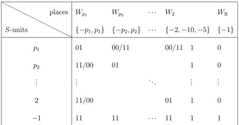
Table 3.1: A boxed code
H H
H H
H H
H H
H H
HH
S-units
places Wp1 Wp2 · · · W2 WR
{−p1, p1} {−p2, p2} · · · {−2,−10,−5} {−1}
p1 01 00/11 00/11 1 0
p2 11/00 01 1 0
..
. ... . .. ... ...
2 11/00 01 1 0
−1 11 11 · · · 11 1 1
We will view then×2n binary matrix M in Table 3.1 as an n×n block matrix
˜
M, where each block is a pair of elements (a2i, a2i+1). Properties of this matrix ˜M
is summarized as follows:
(1) The bottom row of ˜M has all entries equal to (11).
(2) All entries of the last column of ˜M equal the (10) pair except for the (11) in
the final row.
(3) The diagonal elements of ˜M are all (01) except for the final diagonal entry,
which is equal to (11).
We say that a block matrix having properties (1) - (4) ishalf-boxed. We will say
that ˜M is boxed if the following is also true:
(5) For all (n−1)≥i > j ≥1,bij +bji = (11).
By definition, a boxed matrix has rank n and its rows are orthogonal to each
other in the Euclidean pairing. Thus it is a generator matrix for a binary self-dual
code.
The fact that the image of Φ(Z∗S/2) in W is a boxed matrix is a straight
for-ward observation. In particular, property 5 follows from Gauss’s law of quadratic
reciprocity. Thus part (b) in Theorem 3.3.1 is proved.
There is also a partial converse to the above statement,
Lemma 3.3.2. IfM˜0 is half-boxed, and its row vectors are orthogonal to each other, then condition (5) is automatically satisfied, i.e. M˜0 is boxed.
Proof. Taking the product of the i-th row and the j-th row in a half-boxed matrix
(i, j < n, i 6=j) , the products of identical pairs are 0 in F2. Thus if the two rows
are orthogonal, we have bij ·(01) +bji·(01) + (10)·(10) = 0, thus bij+bji= (11).
Now we proceed to prove part (c) of Theorem 3.3.1.
We begin by saying the word of all-ones (denoted ¯1) belongs to every binary
self-dual code C, since ¯1 is orthogonal to all vectors of even weight. Suppose now
last row of M is ¯1. Observe that elementary row operations on M correspond to
a change of basis for the code C. Column permutations send C to an equivalent
code. We will show by induction on n that after applying a sequence of elementary
row operations and column permutations to M, one can make the associated block
matrix ˜M into half-boxed form. We will in fact show that this can be done without
ever adding another row to the final row ¯1 ofM. This will prove the theorem, since
the above operations lead to codes equivalent to C by definition.
Forn = 2 our claim is obvious. Now suppose n >2, M is the generator matrix
for a self-dual code C of length 2n and that the last row of M is ¯1. As the rows of
M have full rank, the top row is neither all-zeros ¯0 nor ¯1. Therefore the columns
of M can be permuted so that the pair on the upper-left corner of ˜M is (01). M˜
has the following form:
Table 3.2: Block form of ˜M
01 u
w M0
In the above table w is a column block-vector of length n−1, u is a row
block-vector with the same number of pairs, and M0 ∈ M at(n−1)×(2n−2). By adding the
top row of ˜M to the j-th row if necessary, where 2 ≤ j < n, we can assume that
w consists only of identical pairs. Under this hypothesis, it is easy to check that
bottom row. By the induction hypothesis, M0 can be turned into half-boxed form
by applying column permutations and row operations while keeping the bottom
row. These same operations can be applied to the augmented matrix M, leading to
a matrix whose lower right cornerM0 is in half-boxed form; the column block-vector
w consists of identical pairs; the bottom row of ˜M remains ¯1.
Now we need to modify the top row u. Note that all diagonal entries of ˜M0 are
all of the form (01) except in the bottom row, and all other pairs in ˜M0 are identical
pairs except in the last column. Therefore the top row of ˜M can be added to by the
2rd through (n−1)th row in such a way that all pairs of u become identical pairs
except possibly for the last pair. During these operations, only identical pairs have
been added to the upper-left corner of M, thus it is either 01 or 10. As the weight
of this first row is even, the last pair in u should also be either 01 or 10. Adding
the bottom row to the top row if necessary, the last pair in u is 10. Finally, if the
upper-left corner of M is 10, it can be turned into 01 by permuting the first two
columns of M. The block matrix ˜M is now in half-boxed form. Moreover, it is in
fact boxed by Lemma 3.3.2.
To complete the proof of (c), we only need to show that every boxed matrix ˜M
can be realized by the Hilbert code associated to some set S ={2,∞, p1, . . . , pn−2}.
To specify the odd pi we begin by requiring their classes in Q∗2/2 ×R
∗/2 as in
the last two block columns of ˜M. This can be done with pi congruent to 3 mod
1≤j < i≤n−2 according to the entrybij in ˜M. After this we have specified the
lower triangular part of a boxed matrix. By Gauss’s quadratic reciprocity, the image
of these S-integers actually give a boxed matrix ˜M under our basis for the Hilbert
symbols. Moreover, by the equidistribution of prime numbers in congruence classes,
each self-dual code can be realized by this construction with an infinite number of
distinct sets of places S.
Example 3.3.3. When S ={∞,2,3,7}, one gets the Hamming code A8.
When
S ={∞,2,7,19,31,131,179,367,883,1223,1307,39079}
one gets the Golay code G24. 4
3.4
A Random Generation Algorithm
The analysis of the previous section hints at an algorithm to generate all equivalence
classes of binary self-dual codes of any fixed length 2n. Namely, one can assign
identical pairs bij in a block matrix ˜M for 1 ≤ i < j ≤ n−1. Then ˜M can be
completed to a boxed matrix which gives a binary self-dual code. Since the pairs
bij for 1 ≤i < j ≤n−1 can be either (11) or (00) freely at will, the algorithm can
either exhaust all the 2n 2−n
2 possibilities, or it can decide bij by a coin tossing. The
advantages of both algorithms are that they are not recursive on n.
generated; or to determine if two codes generated in this way are equivalent or not.
Due to the exponential complexity in these two bottle-necks, we are more interested
in the random algorithm than the exhaustive one. In fact, the random algorithm
can quickly generate non-trivial (i.e. not a direct sum of codes of smaller length),
and theoretically every binary self-dual codes of length 2n.
As toy examples, we generated all binary self-dual codes of length less than 26
by implementing the random algorithm in MATLAB. For simplicity, we count the
weight distribution of each outcome and compare it with the known table.
Remark 3.4.1. In view of the connection between self-dual codes and unimodular
lattices as stated in [KKM91], our algorithm also gives a quick way to construct a
large class of unimodular lattices. ♦
Interesting questions arise in the random generation algorithm. Suppose we
assign the identical pairs bij by independently tossing a coin, what is the probability
of generating a certain equivalence class of codes? Suppose we assign the pair to be
(11) when the coin tossing produces a head. The probability of producing a head
by the coin isθ. Whenθ = 12 andnis small, experiments show that this probability
is very close to the true densities pC of the equivalence classes in T2n defined in
Equation 2.2.2.
In fact, denote the set of binary self-dual codes that have a boxed generator
by
˜
pC =
|CE ∩D2n|
|D2n|
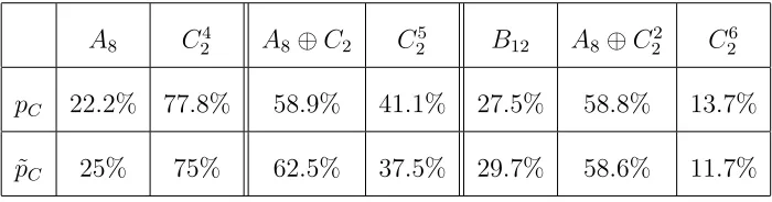
Table 3.3 compares pC and ˜pC for codes of length 8, 10, 12 where we adopt
notations for some codes of small length from [Ple72]
Table 3.3: Comparison of densities in length 8, 10, 12
A8 C24 A8 ⊕C2 C25 B12 A8⊕C22 C26
pC 22.2% 77.8% 58.9% 41.1% 27.5% 58.8% 13.7%
˜
pC 25% 75% 62.5% 37.5% 29.7% 58.6% 11.7%
When the code length grows slight bigger, say 2n= 18 and 20, then to calculate
˜
pC would require a non-trivial amount of work. Therefore, for each length, we run
a Monte-Carlo simulation by letting MATLAB randomly generate 10000 codes and
count the frequencies that each equivalence class shows up:
Table 3.4: Comparison of densities in length 18
H18 F16⊕C2 I18 D14⊕C22 B12⊕C23 A8⊕C25 · · ·
pC 47.30% 26.60% 12.16% 8.69% 3.55% 0.76% · · ·
˜
pC 48.97% 26.18% 11.71% 8.45% 3.18% 0.64% · · ·
In Table 3.4 and 3.5, we did not complete the list when pC and ˜pC gets small.
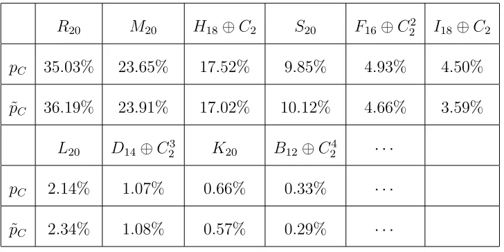
Table 3.5: Comparison of densities in length 20
R20 M20 H18⊕C2 S20 F16⊕C22 I18⊕C2
pC 35.03% 23.65% 17.52% 9.85% 4.93% 4.50%
˜
pC 36.19% 23.91% 17.02% 10.12% 4.66% 3.59%
L20 D14⊕C23 K20 B12⊕C24 · · ·
pC 2.14% 1.07% 0.66% 0.33% · · ·
˜
pC 2.34% 1.08% 0.57% 0.29% · · ·
not seem a coincidence. Based on Proposition 2.2.2, most codes have pC equals to
(2n)!
|T2n|, we ask the following question:
Question 3.4.2. When n→ ∞, what is the behavior of ˜pC for most codes of length
2n?
In the above we have only considered random generation of codes based on a
fair coin tossing, when experiments show that ˜pC is quite close to pC. However, we
can also use a biased coin with probability θ for a head, and denote the probability
for a code C in the algorithm by ˜pθ,C. An easy observation is that given a boxed
matrix M, one may modify the first n −1 rows by adding the bottom row ¯1 to
them. Thus we have a simple observation:
Proposition 3.4.3.
∀C, p˜θ,C = ˜p1−θ,C
For example, one may ask does θ = d2n
2n give a higher probability of producing extremal codes than θ = 12? In general, we propose the following question:
Question 3.4.4. Is there a function θ(n), such that for codes of length 2n, using a
biased coin with probability θ(n) for a head will most likely to produce extremal
codes?
Chapter 4
Construction G
In Chapter 4 and 5 we shift gears and mainly consider questions of an arithmetic
nature that arise in the search for binary self-dual codes. The construction in this
chapter uses duality theorems in ´etale cohomology over some arithmetic schemes.
It is named Construction G where G stands for the word geometry.
In section 4.1, we will restate the Hilbert symbol pairing in Construction Qfor
a general global field in the cohomological language, and give it a new proof in
Proposition 4.1.3 using Artin-Verdier duality. Compared with section 4.2, this is
the “relative dimension zero” case. Towards the end of this section, an interesting
question is asked in Question 4.1.6, relating the statistical behavior of codes in the
construction to the quadratic residues of S-units in the field. In Example 4.1.7, by
choosing fibers over different primes in a curve overZ, Construction G is related to
In section 4.2, an arithmetic duality theorem will be reviewed over an arithmetic
scheme of positive relative dimension over the ring of integers of a totally imaginary
number field. In our construction for a triple (W, E, V) of a binary self-dual code,
W will be the middle dimension cohomology space of an arithmetic scheme;V will
be a half-dimensional subspace inside W which is self-orthogonal with respect to a
non-degenerate bilinear pairing coming from the Yoneda-pairing on the cohomology
space. In general, whether the Yoneda-pairing on W is a Euclidean pairing is an
interesting question, which we discuss in Example 4.2.5 and also come back to in
Example 5.6.5.
4.1
Arithmetic Duality of Global Fields
For a scheme X, we will denote the category of sheaves of abelian groups on the
small ´etale site Xet by Sh(X). When R ∈ Sh(X) is also a sheaf of rings, the
sheaf of R-modules is denoted Sh(X, R). We will mostly be interested in the case
when R is the constant sheaf Z/2. When K is a field, it is well known that there
is a canonical equivalence of categories between Sh(SpecK) and the category of
discrete Gal(K) modules with a continuous Galois action [Sha72, Proposition 71].
Under this equivalence, ´etale cohomology groupsHet∗(SpecK,F) correspond to the
Galois cohomology groups H∗(K, M od(F)), whereM od(F) is the Gal(K) module
associated to F. In this thesis we will abuse these two notations and simple put
Let K be a global field of characteristic different from 2. When v is a place
of K, the completion of K at v is denoted Kv. When v is real Kv = R, we will
consider the Tate (modified) cohomology groups Hb∗(Z/2, M od(F)) [Ser62]. When
v is complex this cohomology space is 0. When v is a finite place, there is the local
Tate duality:
Theorem 4.1.1 (Tate). Suppose Kv is a non-archimedean local field of
character-istic different from2. Given a locally constant constructible sheafF ∈Sh(Kv,Z/2),
define its dual sheaf by FD :=Hom(F, µ
2).
Hi(Kv,F)×H2−i(Kv,FD)→H2(Kv, µ2) =Z/2 (4.1.1)
is a perfect pairing of F2 vector spaces.
We refer to [Mil06, Chapter II] for the definition of a constructible sheaf. When
K is a number field, let OK be the ring of integers of K and let X = Spec(OK).
When K is a global function field, letX be a smooth projective curve with function
field K. U ⊂ X is an open subscheme. S = S∞ tSf is a set of places of K,
where Sf consists of the places determined by the primes in the complement of U,
S∞ contains all of the infinite places of K. For F ∈ Sh(X), denote Hc∗(U,F |U)
the cohomology groups with compact support, where we follow the convention in
[Mil06, section II.2] and cite the following long exact sequence:
· · ·Hcr(U,F |U)→Hr(U,F |U)→ X
v∈S
Hr(Kv,FKv)→H
r+1
There is a global counterpart of the local Tate duality, called the Artin-Verdier
duality [Mil06, section II.3]. WhenSf contains all places with residue characteristic
2, 2 is invertible on U. Under this condition, Artin-Verdier duality for Sh(U,Z/2)
says:
Theorem 4.1.2 (Artin-Verdier). For a locally constant constructible sheaf F ∈ Sh(U,Z/2),
Hetr(U,F)×Hc3−r(U,FD)→H3
c(U, µ2)∼=Z/2 (4.1.3)
is a perfect pairing of F2 vector spaces.
The local Tate duality and Artin-Verdier duality are analogous to the Poincar´e
duality on a topological manifold. When 2 is invertible on U, all the Tate twist µ⊗2i
for i ≥ 0 and their duals can be canonically identified with µ2. We have our first
proposition in Construction G:
Proposition 4.1.3. The image of the restriction homomorphism
Φ :Het1(U, µ2)→ ⊕v∈SHet1(Kv, µ2)
is its own orthogonal complement with respect to the non-degenerate bilinear product
⊕v∈SHet1(Kv, µ2)
× ⊕v∈SHet1(Kv, µ2)
→ ⊕v∈SHet2(Kv, µ2)
δ2
−→Hc3(U, µ2)∼=F2 (4.1.4)
which is the Yoneda-pairing composed with the boundary map in Equation 4.1.2. In
Proof. For a finite place v, by the local Tate duality 4.1.1
H1(Kv, µ2)×H1(Kv, µ2)→H2(Kv, µ2) (4.1.5)
is a non-degenerate bilinear pairing. For a real v, this is also true. The fact that
δ2 in Equation 4.1.4 amounts to taking summations is proved in [Mil06, II.2]. It
is straightforward to see that the direct sum of the non-degenerate bilinear
prod-uct strprod-uctures on each space H1(K
v, µ2) gives a non-degenerate bilinear product
structure on ⊕v∈SH1(Kv, µ2), as in Equation 3.3.1.
Now we prove that the image of
Φ : H1(U, µ2)→ ⊕v∈SH1(Kv, µ2)
is its own orthogonal complement with respect to the product in 4.1.4. This is
a pretty standard exercise in linear algebra. For ease of notation, denote A =
H1(U, µ
2),B =⊕v∈SH1(Kv, µ2) andC =Hc2(U, µ2). The pairing in Equation 4.1.4
identifies the linear dual ˇB = HomF2(B,F2) withB. The perfect pairingA×C→F2
in 4.1.2 identifies ˇA with C. From 4.1.2 for r= 1 we have an exact sequence
A−→Φ B−→Ψ C (4.1.6)
Here the above pairings identify the map Ψ : ˇB →B →C= ˇA with the dual ˇΦ
of Φ. Hence
dim(coker(Φ)) = dim(ker( ˇΦ)) = dim(ker(Ψ)) = dim(image(Φ))
where the last equality follows from Equation 4.1.6. Thus dim(image(Φ)) = 12dim(B).
the product 4.1.4 on B is non-degenerate. We have the commutative diagram:
A×A −−−→∪ H2(U, µ 2)
yΦ×Φ
y
B×B −−−→ ⊕∪ v∈SH2(Kv, µ2)
(4.1.7)
Since the composition of the maps
H2(U, µ2)→ ⊕v∈SH2(Kv, µ2)
δ2
−→Hc3(U, µ2)
is 0 by the exactness of the sequence, we have proved image(Φ) ⊆image(Φ)⊥.
Remark 4.1.4. For a triple (W, V, E) to be a binary self-dual code, we need that the
non-degenerate bilinear product on W is Euclidean, where E is a Euclidean basis.
Apply Galois cohomology to the Kummer sequence
0→µ2 →Gm
×2
−→Gm →0 (4.1.8)
By Hilbert’s Satz 90H1(K,
Gm) = 0, therefore it is shownH1(Kv, µ2) =Kv∗/2. The
pairing 4.1.5 is just the Hilbert symbol pairing [Ser62, Chapter XIV]. By Corollary
3.2.3 Wv :=H1(Kv, µ2) is Euclidean if and only −16∈(Kv∗)2. For a finite extension
Kv/Q2,dimF2K
∗
v/2 = 2 + [Kv :Q2] by the structure theorem of local fields [Neu99,
Proposition 5.7, Chap II]. Combined with Corollary 3.2.3 and the discussion in
Section 3.2, whenWv is Euclidean, it showsEv is unique up to permutations if and
only if the residue characteristic of v is different from 2 orKv =Q2. After choosing
a basis Ev for each Wv, we always takeE =tv∈SEv.
By Albert’s Theorem 3.2.2, when some subspaces Wv are alternate and some
However, there will be no natural way to choose a Euclidean basis E in W up to
permutations unless dimF2W ≤3. By Section 2.2, the combinatorial properties of
a binary self-dual code depends on the choice ofE up to permutations. Thus unless
there is a natural way to pick a basis E, a binary self-dual code (W, V, E) is not
well-defined. ♦
Example 4.1.5. Suppose K is a number field and X = Spec(OK). Taking
cohomol-ogy of the Kummer sequence 4.1.8, it produces
0→ OK,S∗ /2→H1(U, µ2)→P ic(U)[2] →0
where P ic(U)[2] denotes the two torsion elements in the abelian group P ic(U).
When P ic(U) is odd, O∗
K,S/2 = H1(U, µ2). The image of Φ in Proposition 4.1.3 is
the diagonal image O∗
K,S/2→ ⊕v∈SKv∗/2 as in ConstructionQ. We will show that
Φ is injective under our assumption thatS contains all the infinite places and finite
places v|2.
By 3.1.1h1(U, µ
2) =dimF2O
∗
K,S/2 = |S|.
When v|2, h1(K
v, µ2) = 2 + [Kv :Q2]. When v -2∈Sf, h1(Kv, µ2) = 2. When
v is real, h1(Kv, µ2) = 1. When v is complex it is trivial. Therefore
X
v∈S
h1(Kv, µ2) =
X
v|2
(2 + [Kv :Q2]) + (
X
v-2,v∈Sf
2) +r1 = 2r2+r1+ 2|Sf|+r1 = 2|S|
(4.1.9)
where r1 is the number of real places,r2 the number of complex places. By
Propo-sition 4.1.3, 12dimF2W =dimF2image(Φ) =h1(U, µ
When P ic(U)[2] 6= 0 the two-torsion elements in the Picard group are also
involved in the construction. However this is related to the odd Picard number
case. Suppose U0 ⊂U is a smaller open subscheme, the map Φ factors through
H1(U,Z/2)→H1(U0,Z/2)→ ⊕v∈SH1(Kv, µ2)
whence we can take a small enough U0 such that such that P ic(U0) is odd.
In general, the diagonal image Φ : O∗
K,S → ⊕v∈SKv∗/2 has more complicated
patterns than a boxed-matrix as in table 3.1. From the above discussion, if for
all v|2 Kv = Q2, a binary self-dual code (W, V, E) is well defined. However, when
[K : Q] > 0 it is usually hard to give a combinatorial description of image(Φ),
besides the fact that it is a binary self-dual code. This is related to the problem
of giving an elementary description of a “quadratic reciprocity law” for v|2 in K,
see [Lem00] for an overview. Characterizing the image of Φ also concerns the
behavior of quadratic residues of the S-units in K. It would be interesting to see
how a viewpoint from the binary self-dual code structure can help us probe these
problems. For example, one can ask the following question:
Question 4.1.6. Consider the set of number fieldsK where 2 splits completely. Fix
the number of embeddings r1, r2 of K and let the discriminant disc(K) grow by
magnitude. If Sf contains only v|2, the length of the code is fixed to be 4r1 + 6r2
by Equation 4.1.9. What is the frequency that a certain equivalence of codes of this
length is generated? How is this frequency related to the density ˜pθ in section 3.4?
Example 4.1.7 (Local-Global Codes). Consider the global function fieldFq(T), where
q = pn ≡ 3 mod 4, T is a transcendental parameter. X = P1Fq. Let S =
{1
T, g1(T),· · · , gn−1(T)}where eachgi(T) is a monic irreducible polynomial inFq[T]. The image of Φ is given by the global S-units h−1, g1(T),· · ·, gn−1(T)i in W =
⊕v∈SKv∗/(Kv∗)2. Suppose each gi(T) has odd degree, then the Hilbert symbol
pair-ing W×W →F2 has a natural choice of Euclidean basis. It is not hard to see that
the diagonal image of Φ is also described by a boxed-matrix in table 3.1.
WhenFq =Fp is a prime field, X can be considered to be the fiber over SpecFp
in P1
Z. Consider some horizontal divisors defined by linear integral polynomials
gi(T) = T −ai onP1Z, where ai ∈ Z. The pull-back of these horizontal divisors on
X are rational points defined by gi(T) mod p. When |p|> max1≤i≤n−12|ai|, gi(T)
mod p will give distinct rational points on X. In the boxed-matrix description
of the resulting code, the pair bij is determined by the Legendre symbol ( ai−aj
p ).
By Gauss’s quadratic reciprocity, the Legendre symbol is also determined by the
congruence conditions of p mod the prime factors in (ai − aj). For simplicity,
assume for all sets of indices {i, j}, there is an odd prime number fij and n, such
that fijn|(ai−aj), fijn+1 - (ai −aj), and fij - (ai0 −aj0) when {i, j} 6= {i0, j0}. Now
let the prime number pgrow by magnitude in the congruence class of 3 mod 4. By
the equidistribution of the prime numberp in the congruence classes mod thefij’s,
the Legendre symbol (ai−aj
p ) is 1 or −1 exactly half of the time. Therefore, when
we take X to be the fiber over different prime p ≡ 3 mod 4 in P1
divisors S generate binary self-dual codes like the random algorithm in section 3.4
using a fair coin! 4
4.2
Duality of Arithmetic Schemes
In this section, we will continue the construction from the previous section and
gen-eralize Proposition 4.1.3 to certain arithmetic schemes of positive relative dimension
over X, where X, K, S and U have the same meaning from the previous section.
Recall thatK is a global field of characteristic different from 2 and 2 is invertible on
U. Let π : Y →X be an integral, projective scheme over X of relative dimension
d > 0. Suppose Y is smooth over an open subschemeU ⊆X and its generic fiber
YK is geometrically irreducible. First we recall the following generalization of the
local Tate duality [Sai89]:
Proposition 4.2.1. Kv is a non-archimedean local field of characteristic different
from 2. Given a locally constant constructible sheaf F ∈Sh(YKv,Z/2),
Hi(YKv,F)×H
2d+2−i(Y Kv,F
D)→H2d+2(Y
Kv, µ2) = Z/2 (4.2.1)
is a perfect pairing of F2 vector spaces.
When v is a complex place, the Tate cohomology groupsHbi(C, M) = 0 for any
module M and i∈Z. Therefore for a complex variety π :Z →C and F ∈Sh(Z),
b
Hi(Z,F) = b
Hi(
C, Rπ∗F) = 0. Proposition 4.2.1 is trivially satisfied.
Proposition 4.2.2. Given a locally constant constructible sheaf F ∈Sh(Y,Z/2),
Hetr(YU,F)×Hc3+2d−r(YU,F∨)→Hc3+2d(YU, µ2)∼=Z/2 (4.2.2)
is a perfect pairing of F2 vector spaces.
Using Proposition 4.2.1 and 4.2.2, the following is a corollary of Proposition
4.1.3:
Corollary 4.2.3. When K is a totally imaginary number field or a global function field of characteristic different from 2, the image of the restriction homomorphism
Φ : Hetd+1(YU, µ2)→ ⊕v∈SHetd+1(YKv, µ2)
is its own orthogonal complement with respect to the non-degenerate bilinear product
⊕v∈SHetd+1(YKv, µ2)
× ⊕v∈SHetd+1(YKv, µ2)
→ ⊕v∈SHet2d+2(YKv, µ2)
δ2d+3
−→Hc3+2d(YU, µ2)∼=F2 (4.2.3)
which is the Yoneda-pairing composed with taking summations.
Remark 4.2.4. The reason we do not consider the case whenK has a real embedding
is that although Proposition 4.2.2 remains valid, Proposition 4.2.1 is in general not
true for a real local field, see [Cox79]. ♦
When d = 1, V is the diagonal image Φ : H2(YU, µ2)→
P v∈SH
2(Y
Kv, µ2). By
the Kummer sequence, H2(Y, µ
2) can be computed by
whereBr(Y) :=H2(Y,
Gm) is the cohomological Brauer group. An explicit
descrip-tion of the map Φ would be very interesting, which we leave for further study.
In general, it is not an easy problem to determine if the Yoneda-pairing
h,i:Hd+1(YKv, µ2)×H
d+1
(YKv, µ2)→H
2d+1
(YKv, µ2) (4.2.4)
used in Corollary 4.2.3 is Euclidean or alternate, as is illustrated in the following
example.
Example 4.2.5. Consider the case YKv = P
1
Kv. The Hochschild-Serre spectral
se-quence is often used to calculate H∗(PK1v, µ2):
Hi(Kv, Hj(PK1v, µ2))⇒Hi+j(PK1v, µ2) (4.2.5)
where Kv denotes an algebraic closure of Kv. This spectral sequence is
multiplica-tive, in the sense that there is a pairing on the E2 page:
Ep1,q1
2 ∪E
p2,q2
2 →E
p1+p2,q1+q2
2
which when passing toE∞is compatible with the cup product structure onH∗(PK1v, µ2).
It is easy to see that the spectral sequence 4.2.5 degenerates on the E2 page.
De-note E22,0 = {0, y} ,→ H2(P1
Kv, µ2) = {0, x, y, x+y} =:Wv. E
0,2
2 can be naturally
identified with the quotient {0,x¯} of Wv modulo the subspace{0, y}.
Since the pairing h,i on Wv is non-degenerate, the fact that y∪y ∈ E24,0 = 0
implies hx, yi= 1 is non-trivial. Thus on the quotient spaceE20,2,
The multiplicative structure onE2of 4.2.5 alone does not suffice to determine if 4.2.4
is Euclidean or alternate. In Example 5.6.5, we will prove the following theorem
using techniques from an equivariant ´etale cohomology theory.
Theorem 4.2.6. The cup product pairing 4.2.4 is alternate when YKv =P
1
Kv or EKv,
where EKv is an elliptic curve with good reduction over a local field Kv with residue
characteristic different from 2.
Chapter 5
The Equivariant Construction
Ever since the 1950s, equivariant cohomology has been a powerful tool in the study
of group actions on spaces. Borel defined an equivariant cohomology for the action
of a compact group G on a topological space [Bor60]. In [Gro57], Grothendieck
defined an equivariant sheaf cohomology for the action of a discrete group. For a
finite group, the Borel construction can be generalized to actions on sheaves and it
coincides with Grothendieck’s equivariant sheaf cohomology [Sti79]. In this
chap-ter, we will transplant certain statements for a finite group action on a finite CW
complex to an action on equivariant ´etale sheaves over a scheme. For an application
to the construction of binary self-dual codes, we will mainly be concerned with the
case G=Z/2.
In Section 5.1, we will follow [AP93, Chapter I] and review the set-up of a
use a minimal Hirsch-Brown model for an equivariantG-complex. In section 5.2, we
will specialize to consider equivariant ´etale sheaves over a scheme, and recall Morin’s
construction of a modified equivariant ´etale cohomology. In section 5.3, we prove
a “Smith-type inequality” 5.3.1 using Theorem 5.3.3 from [Mor08]. We will call it
the maximal case when 5.3.1 is an equality. In the maximal case for a Z/2 action
on a scheme Y where 2 is invertible, cohomological duality statements on Y can
be utilized to construct binary self-orthogonal spaces, following [Pup01]. In section
5.5 we compare the Equivariant Construction and Construction G in the previous
chapter. In Example 5.5.4, the reader will find that while the two constructions
give the same underlying vector spaces for a code, their product structures are not
necessarily the same. In the final section 5.6, we provide some more discussions
on the maximum condition 5.3.8. In particular, in Example 5.6.5 the maximum
condition is met, and the deformation trick can be used to prove Theorem 4.2.6.
5.1
Cohomology of a
G
-Complex
Let G be a finite group and k be a field. C∗ is a bounded below cochain complex
of k[G]-modules, we will call C∗ a δgk[G]-Mod, where δ : Ci → Ci+1 is the G
-equivariant differential. Similarly, we will call a bounded above chain complex of
k[G]-modules a∂gk[G]-Mod. Recall the following construction of the hyper-derived
k,
· · · Ei → Ei−1· · · → E1 → E0 →k →0
Define βGn(C∗) := Πi+j=nHomk[G](Ei, Cj). Equivalently, define the dual
com-plex E∗ as Ei := Hom
k[G](Ei, k[G]), since C∗ is bounded from below, βGn(C
∗) ∼
=
⊕i+j=nCj⊗k[G]Ei. ThenExtnk[G](k, C
∗) :=Hn(β∗
G(C
∗)). We will follow [AP93] and
call this group HG∗(C∗). Recall [Ben98, 3.2], the cup product
HGi (C∗)⊗HGj(S∗)→HGi+1(C∗⊗S∗)
is associative and graded-commutative. When there is an associative,
graded-commutativeδgk[G]-Mod morphismC∗⊗C∗ →C∗,HG∗(C∗) is a graded-commutative
algebra overHG∗(k). For our purpose, we will only consider the case whenG=Z/2
and k is a field of characteristic 2. Thus it is not necessary to distinguish between
left and right G-actions and the ± sign doesn’t matter. Following [AP93, Chapter
I], we will pick a particular (minimal) resolution E∗ such that for any δgk[G]-Mod
C∗, βG∗(C∗) is already a right graded βG∗(k)-module on the cochain level.
Denote G = Z/2 = {1, g}. Take E∗ = k[G]⊗W∗, where each graded piece
Wn is freely generated by {wn} as a k-module. The G-equivariant differential δ is
defined by δwn := (1−g)wn+1. Under this E∗, βn
G(k) is generated as a k-module
by wn⊗k[G]1∈ En⊗k. The differential on βGn(k) is trivial, and βG∗(k)∼=H∗(G, k)
as δgk-Mod. βG∗(k) obtains a commutative ring structure from HG∗(k), which is
Consider the δgk-Mod βG∗(C∗) =C∗ ⊗k[G]E∗. Since tensor product is
commu-tative for graded k-modules,
C∗⊗k[G]E∗ ∼=C∗⊗k[G](k[G]⊗W∗)∼= (C∗⊗k[G]k[G])⊗kW∗ ∼=C∗⊗kW∗
Under this isomorphism, C∗⊗W∗ obtains a differential δefrom βG∗(C∗).
Lemma 5.1.1. [AP93, Proposition 1.3.4] The cochain complex βG∗(C∗) is a free graded right k[t]-module isomorphic to C∗⊗k[t], and the differential eδ on C∗⊗k[t]
is right k[t]-linear.
Remark 5.1.2. Multiplication of k[t] on the left of C∗ ⊗k[t] is associative only up
to cochain homotopy, loc. cit. ♦
We will call a graded k[t]-module with a k[t]-linear differential a δgk[t]-Mod.
Explicitly, the differential eδ on C∗⊗k[t] is given by
e
δ(c⊗1) =δ(c)⊗1 +c(1−g)⊗t (5.1.1)
In particular,eδis not the usual differential of the tensor product of twoδgk-ModC∗
and k[t], a phenomenon which was already observed in [Bro59]. In general, given a
δgk-Mod (C, δ), a δgk[t]-Mod (C⊗k[t],eδ) is called adeformation of (C, δ) if
e
δ(c⊗1) =X i
bi⊗ti
where b0 =δ(c). We denote (C⊗k[t],eδ) by C∗⊗ek[t] to emphasis the deformation.
Since k is a field, all exact sequences of k-modules split (non-canonically), by
coho-mology group. Therefore a δgk-ModC∗ is homotopic to H∗(C∗) with trivial
differ-ential. By [AP93, B.2.4], C∗⊗ek[t] is homotopic to H
∗(C∗)
e
⊗k[t], which is called the
minimal Hirsch-Brown model for βG∗(C∗).
For applications in the next section, we also consider the localization at t of a
δgk[t]-ModM∗. As usual, given a gradedk[t]-moduleM∗ =⊕n∈ZM
n, the degreen
piece of its localization at the homogeneous ideal (t) is given by⊕j∈ZMn−j⊗tj. We
extend the differentialk[t,1t]-linearly, and denote this localization byM∗⊗k[t]k[t,1t].
5.2
Equivariant Etale Sheaves
In this section we will recall some facts about the category of equivariant ´etale
sheaves on the ´etale site of a locally noetherian scheme Xet, denoted Sh(X, G). In
this section, G is a finite group acting on X, and F is a sheaf on Xet.
Definition 5.2.1. A G-linearization of F is a family of morphismsϕσ,:σ∗F → F
indexed by σ∈G that satisfy the following conditions:
• ϕ1 =Id.
• ϕτ σ =ϕτ ◦τ∗(ϕσ).
A G-linearized sheaf F is called an equivariant G-sheaf, F ∈ Sh(X, G). A
morphism of G-sheavesα :F → L onXet is a morphism of sheaves that commutes
HomSh(X)(F,L) by
σ(α) :=ϕL,σ◦σ∗(α)◦ϕ−F1,σ
Then HomSh(X,G)(F,L) is the invariant subgroup under this action. ♦
Sh(X, G) is an abelian category with enough injectives. WhenF is an injective
object in Sh(X, G), it is also injective in Sh(X) [Mor08] and the group of global
sections F(X) is an injective Z[G]-Mod [Gro57, Lemma 4.3.1].
We can apply the construction in the previous section to define equivariant
´
etale cohomology groups of equivariant sheaves. Given a sheaf of k-modules F ∈
Sh(X, G) where k is a field, take an injective resolution I∗ inSh(X, G) and apply
the global section functor. This gives a complex of k[G]-modulesI∗(X):
I0(X)→ I1(X)→ I2(X)· · ·
Define a δgk-ModβG∗(F) whereβGn(F) :=⊕i+j=nHomk[G](Ei,Ij(X)).
Definition 5.2.2. The equivariant sheaf cohomology is defined as HG∗(X,F) :=
H∗(βG∗(F)). ♦
Remark 5.2.3. A standard spectral sequence argument shows thatHG∗(X,F) defined
in this way is equal to Grothendieck’s equivariant cohomology groups H∗(X, G,F),
which are derived functors of F(X)G [Wei94, 5.8]. ♦
In [Mor08] a modified equivariant ´etale cohomology is introduced. Consider a
Definition 5.2.4. DefineβbG∗(F) :=Homk[G](J∗,I∗(X)) where
b
βGn(F) := ⊕i+j=nHomk[G](Ji,Ij(X)). Define HbG∗(X,F) :=H∗(βbG∗(F)). ♦
When G=Z/2, we can choose a (minimal) complete resolution J∗ by splicing
together a (minimal) resolution E∗ and its dual. Under this J∗, the following is a
corollary of Lemma 5.1.1:
Corollary 5.2.5. As a δgk[t,1t]-Mod, βbG∗(F)∼=βG∗(X,F)⊗k[t]k[t,t1]∼=C∗⊗ek[t,
1
t].
By definition, it is obvious that βbGi+1(F) ∼= βbGi (F)⊗k[t,1
t]t and b
HGi+1(X,F) ∼=
b
HGi (X,F)⊗k[t,1
t]t. In particular,Hb ∗
G(X,F) is a free k[t,1t] module.
HG∗(X,−) satisfies the usual properties as a derived functor, and there is a
spectral sequence converging to it:
Hp(G, Hq(X,F))⇒HGp+q(X,F) (5.2.1)
On the other hand, it is also proved in [Mor08] that HbG∗(X,−) satisfies some
nice properties. For example, a short exact sequence of G-sheaves
0→ F1 → F2 → F3 →0
leads to a long exact sequence in HbG∗(X,−). There is also a functorial spectral
sequences converging to HbG∗(X,−), whoseE2 page is given by
b
Hp(G, Hq(X,F))⇒HbGp+q(X,F) (5.2.2)