RESEARCH
Designing minimal microbial strains
of desired functionality using a genetic
algorithm
Govind Nair
1,2, Christian Jungreuthmayer
1,2, Michael Hanscho
1,2and Jürgen Zanghellini
1,2*Abstract
Background: The rational, in silico prediction of gene-knockouts to turn organisms into efficient cell factories is an essential and computationally challenging task in metabolic engineering. Elementary flux mode analysis in combina-tion with constraint minimal cut sets is a particularly powerful method to identify optimal engineering targets, which will force an organism into the desired metabolic state. Given an engineering objective, it is theoretically possible, although computationally impractical, to find the best minimal intervention strategies.
Results: We developed a genetic algorithm (GA-MCS) to quickly find many (near) optimal intervention strategies while overcoming the above mentioned computational burden. We tested our algorithm on Escherichia coli meta-bolic networks of three different sizes to find intervention strategies satisfying three different engineering objectives. Conclusions: We show that GA-MCS finds all practically relevant targets for any (non)-linear engineering objective. Our algorithm also found solutions comparable to previously published results. We show that for large networks opti-mal solutions are found within a fraction of the time used for a complete enumeration.
Keywords: Systems biology, Metabolic networks, Elementary flux modes, Minimal cut sets, Strain optimization
© 2015 Nair et al. This article is distributed under the terms of the Creative Commons Attribution 4.0 International License (http:// creativecommons.org/licenses/by/4.0/), which permits unrestricted use, distribution, and reproduction in any medium, provided you give appropriate credit to the original author(s) and the source, provide a link to the Creative Commons license, and indicate if changes were made. The Creative Commons Public Domain Dedication waiver (http://creativecommons.org/publicdomain/ zero/1.0/) applies to the data made available in this article, unless otherwise stated.
Background
The availability of high amount of biological data has led to the reconstruction of genome-scale metabolic networks for many organisms [1–4] which can be ana-lysed and probed using mathematical and computational
methods [5, 6]. Prominent among these are constraint
based modelling approaches which depend on the stoi-chiometry of the reactions. These include methods like flux balance analysis, FBA, [7] and elementary flux mode
analysis, EFMA [8, 9]. The major difference between
these approaches is that FBA seeks particular flux solu-tions whereas EFMA seeks to describe the entire flux space by enumerating all its elementary and balanced pathways which are called elementary flux modes, EFMs. Thus, the complete set of EFMs describes all possible cel-lular states. The disadvantage is that enumerating all the EFMs of a metabolic network is computationally very
demanding as the number of EFMs explodes with net-work size [10]. However, the ability to enumerate EFMs has been steadily improving [11–14].
An important application of an EFMA is the predic-tion of gene knockouts to turn wild-type organisms into efficient minimal cell factories [15]. The design of effi-cient cell factories is based on the concept of networks of minimal functionality. These are derived from wildtype metabolic networks by keeping typically very few, spe-cifically selected metabolic functions, e.g., EFMs with high yields of products of interest, while diminishing all other unwanted (wildtype) functionality by appropriately selected gene/reaction knockouts. These interventions channel the available carbon flux towards the product of interest. Based on EFMA the concept of constrained minimal cut sets, cMCS can be used to redirect cellular resources towards the product of interest [16]. cMCS are minimal (reaction) knock-out strategies, that disable unwanted EFMs (e.g., low product yield/growth) while the desired EFMs (e.g., high product yield) are preserved.
Open Access
In particular, cMCSs of minimal cardinality are impor-tant as these solutions minimize the experimental effort when knockouts are actually implemented in vivo. Sev-eral methods for the computation of cMCS based on a given EFM spectrum are known [16–18]. Alternatively, cMCS can also be calculated directly without first cal-culating EFMs [19–21]. However, in all these methods, explicit design criteria must be used (e.g. by providing boundaries for the desired minimal product yield). This is problematic in so far as a slight change in the design criteria might lead to large changes in the minimal cardi-nality of the cMCSs, i.e. the minimal number of required knockouts. For example, Trinh et al. [15] optimized E.
coli for ethanol production with seven reaction
knock-outs. Jungreuthmayer et al. [22] on the other hand, were able to design a strain with identical key features and almost identical overall functionality, which required only five reaction knockouts.
If the EFMs are known it is theoretically possible but generally impractical to find all optimal partitions of EFMs and their corresponding cMCSs (of minimal cardi-nality). In a recent work Ruckerbauer et al. [23] approach this problem by first finding the smallest possible cMCS which contributes towards the engineering objective. Then cMCSs of higher cardinality are successively enu-merated such that the engineering objective value is greater than or equal to that of the previous smaller cMCS. This circumvents the problem of large number of binning possibilities but will work, in a reasonable amount of time, only for small scale networks.
Here we present a novel approach which uses a genetic algorithm, GA to “evolve” near optimal solutions from starting sets of randomly partitioned modes. This results in minimal strains such that only that fraction of the total EFMs which contribute towards the design objec-tive are acobjec-tive after deletion of the predicted cMCSs. This approach combines the simplicity of a GA with the power of EFMA and cMCS. The GA not only circumvents the manual partitioning of EFMs but also finds increasingly better solutions in a relatively short amount of time. This method can be used to satisfy not only traditional design objectives like product yield and growth but can also incorporate more complex design objectives like high growth-coupled product yield using minimal number of knockouts or even non-linear objectives.
Preliminaries
Elementary flux modes, EFMs
The material balances in a metabolic network with m
internal metabolites and r reactions in steady state can be represented by
(1)
N·v = 0.
where N is the m×r stoichiometric matrix and v is a flux
vector containing the fluxes through the network and
v∈Rr, i.e., v=(v1,. . .,vr)T. The set of reactions can be partitioned based on thermodynamic constraints into sets of reversible and irreversible reactions. If Irrev is the index set of irreversible reactions,
The support of the flux vector v can be defined as
supp(v) = {j|vj�=0}, which is the set of reaction indices
in v with non-zero flux values. An EFM, e, is a flux vector v�=0 which satisfies (1), (2) and a non-decomposability
condition which states that, there is no non-trivial flux vector w satisfying (1), (2) and whose support is a proper subset of e, i.e., supp(w) ⊂ supp(e). The non-decom-posability condition means that the removal of any sup-porting reaction in an EFM will block a steady state flux through it. The set of all EFMs of a network completely describes the entire metabolic capabilities of the network. Every possible flux through the network can be expressed as a non-negative weighted combination of EFMs with-out cancellation. This means that if the flux through a reaction is 0, then all the contributing EFMs necessarily will have 0 flux through that reaction. For more informa-tion on EFMs, see [24].
We will use the following notation henceforth, E =supp(e). Let E= {E1,. . .,En} represent the full set of
all n EFMs in support notation.
Constrained minimal cutsets, cMCSs
Suppose there are certain network states which need to be suppressed. These states can be represented by a set of EFMs T, where T⊂E. The problem then becomes one of
“killing” all the EFMs in T. This can be done by “knock-ing-out” a cutset C of reactions which will “hit” all of T. That is,
C will be a minimal cut set, MCS, if there is no proper subset B⊂C which satisfies (3) [25].
Suppose that in addition to network states which need to be suppressed, there are certain states which we need to preserve when knockouts are applied (e.g. biomass production and product formation). This can be done using the concept of cMCS [16]. The set of desired EFMs
D corresponds to the network states to be preserved.
Since in general it cannot be expected that an MCS will not hit any of D, we will say that we would like to have at least k EFMs untouched by an MCS where k≤ |D|.
Given an MCS C, let the set of EFMs DC represent D∈D
which survive after applying C,
(2)
vj ≥ 0 ∀j ∈ Irrev.
(3)
∀T∈T, C∩T�= ∅,
(4)
An MCS which satisfies (3) and the following constraint is a cMCS
Thus an intervention problem
is defined by a set of target EFMs T which need to be
“killed” and a set of desired modes D of which at least k have to be “kept”. Several methods to solve (6) are availa-ble [16–18]. Note that D∪T does not necessarily unite to the full set of EFMs since there could be EFMs which we do not want to either kill or keep but instead have a “don’t care” status. However, we do not need to specify such an association since we will not operate on these EFMs. We will operate only on the EFMs we are interested in (D
and T) and do not bother with what happens to the EFMs with “don’t care” status because by definition it wouldn’t matter to us if these EFMs survive or are killed.
In the following we describe a GA to solve the interven-tion problem (6). For simplicity our implementainterven-tion par-titions the complete set of EFMs into D and T and does not make use of the “don’t care” option.
Methods
The EFM kill/keep problem
Equation (6) allows to search for cMCS which keep cer-tain EFMs and kill others. However, it is not intuitive which EFMs to keep and which to kill in order to mini-mize the cardinality of the cMCSs. Thus the question arises: What is the best partitioning of EFMs in order to reach a specific engineering objective? Even in a modest sized network, the possible combination of EFMs to keep or kill is very large. For example, in a small scale network with 5000 EFMs, the number of possible kill/keep combi-nations is 25000. It is practically impossible to explore all
points in such a large solution space. Therefore, it makes sense to utilize a program that finds the best set of EFMs to keep, and the corresponding cMCSs which will achieve this for a given an engineering objective [23]. We do this using a GA, the working of which is described below.
The genetic algorithm, GA
GAs are heuristics inspired by the theory of evolution, generally used when the extreme of the function can-not be analytically established or when it is impractical to search the whole solution space. GAs work on prob-lems by encoding possible solutions into a population of individuals. These individuals are chromosome like data structures which are iteratively refined to “evolve” better solutions by applying strategies inspired by Darwinian evolution [26–29]. In our implementation each individ-ual represents an intervention problem (6).
(5)
|DC| ≥k.
(6)
I =I(T,D,k)
Given a population size p, we randomly generate indi-viduals Si= {si1,. . .,sni}, 1≤i≤p, where each element s
j i of Si indicates if the EFM Ej is present (sji=1) in the indi-vidual Si or not (sji =0). Thus each individual Si codes an intervention problem (6) with
where wk ∈ [0, 1] is a freely adjustable GA parameter. sji
-values are assigned randomly but we provided for the possibility to pre-process EFMs such that EFMs with desirable characteristics have a higher chance of being 1. For example, suppose a cell is described by the following set of EFMs {E1,. . .,E7}, where only E1, E3 and E7 support
product formation. If we want to optimize for product formation, we clearly do not want to keep the non-pro-ducer. So we choose sij such that undesirable states never
get selected. In our example possible randomly selected individuals could look like S1= {1, 0, 1, 0, 0, 0, 1}, S2= {1, 0, 1, 0, 0, 0, 0}, etc. while {1, 1, 1, 0, 0, 0, 1} would
not be generated because it includes E2 which we want
to eliminate. This leads to a significant reduction in the search space. Finally, for each individual Si, cMCS are cal-culated using the MHScalculator [30].
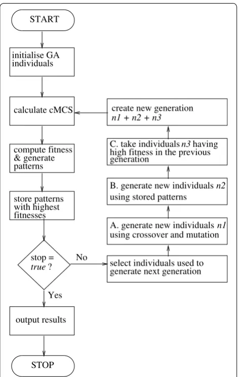
GAs aim to proceed towards better solutions by evalu-ating each individual Si against a fitness function F and selecting the top-performers for procreation. The fitness function reflects the design objective since those are the traits we want to improve. In our implementation indi-viduals are selected for mating using a fitness propor-tionate selection [31]. In addition, we use the concept of “elitism” where a pre-specified percentage of top-per-formers will propagate into the next generation without any modification as shown in Fig. 2c. This guarantees that the population’s maximum fitness does not decrease. We
use crossover, mutation [26, 27], and random selection
based on previous information about surviving EFMs to produce a new generation of individuals. These mecha-nisms are explained below.
Crossover
We take two parent individuals, S1 and S2, and randomly
exchange their elements to create two new offspring S3
and S4. We implemented the following three standard
types of crossovers. For 1point crossover, generate a ran-dom integer rc, 1≤rc<n for each pair of parents, then
the offspring of crossover are S3= {s11, ...sr1c,src
+1 2 , ...sn2}
and S4= {s12, ...src 2,src
+1
1 , ...sn1}, (see Fig. 2a). In 2point
crossover, two random integers rc1,rc2, 1≤rc1<rc2<n are generated for each pair of parents. The offspring in this scenario are S3= {s11, ...s
rc1 1 ,s
rc1+1
2 , ...s
rc2 2 ,s
rc2+1
1 , ...sn1} and
(7)
Ii=Ii[T(Si),D(Si),k(Si)],
withT(Si)= {Ej|sji=0}, D(Si)= {Ej|sji=1},
k(Si)=wk|D(Si)|
S4= {s12, ...src1 2 ,s
rc1+1 1 , ...s
rc2 1 ,s
rc2+1
2 , ...sn2}. In uniform
cross-over, for each EFM a random number 0≤ruj <1 is
gen-erated and the offspring are S3= {sj1 ifruj <0.5 elsesj2}
and S4= {s2j ifrju<0.5 elsesj1}.
Mutation
Given an individual S1 and a random integer r, 1≤r<n , the mutated individual is S2= {si1 ifi�=r, else 1−si1}.
The absolute number of such random integers generated for each individual is given by ρrm, where rm is a freely
adjustable GA parameter, the mutation rate, 0≤rm<1
and ρ the maximum number of EFMs with desirable
characteristics, ρ≤n (see Fig. 2a).
Pattern‑based individual generation
In addition to mutation and crossover we create new individuals based on the fittest patterns. For each indi-vidual S, whose corresponding intervention problem has solution(/s), we generate a “design pattern”, which con-tains only the surviving EFMs,
Given a binary individual S = 1010001, if only EFM 3
and 7 survive the intervention, the resulting pattern will be 0010001. Thus a pattern is a specific strain design for an intervention problem. A solvable intervention prob-lem typically produces more than one solution. There-fore, one individual will usually have more than one pattern associated with it. Since the fitness depends on the surviving EFMs, each pattern will have its own fitness value. Thus one individual may be associated with more than one fitness value. Here, the fitness of an individual S is defined as the fitness of the fittest pattern P.
To create the new individuals, we start by weighting each EFM proportional to the number of times the EFM survived in all previous patterns. Let Pt represent the
entire set of patterns found until a given generation t. The weight wit for an EFM Ei is calculated by
Next we generate a set of desired candidate EFMs by ran-domly selecting a random number of EFMs with non-vanishing wti. Out of these desired candidate EFMs new
individuals were composed by including those candidate
EFMs for which a randomly selected number ri was not
larger than the weight of the corresponding candidate EFM, 0≤ri <maxwt and maxwt is the maximum of all such weights (see Fig. 2b),
(8)
P= {pj|pj=1 ifEj∈DCelsepj =0}.
(9)
wti = |Pt|
j=1
(Pt)i
j.
(10)
Snew= {sinew| ifwti≥ri, sinew=1 elsesinew =0}.
The number of individuals generated by this method can be controlled by the GA parameter ‘new_S’, Table 1. It is a way to consider all good solutions obtained so far and ensures that more EFMs with desirable properties find their way into the set of desired EFMs. This helps the GA to reach the optimum faster.
The GA stops after reaching a pre-specified number of generations or when the maximum fitness doesn’t improve for a given number of generations, outputting all MCSs of minimal cardinality associated with each desired pattern. The schematic of the GA implemented and used here is shown in Fig. 1 along with a small illus-tratory example in Fig. 2.
Implementation
The GA was implemented in Perl http://www.perl.org/. cMCSs were calculated with MHScalculator which is an open source C-program that is freely available [30]. EFMs were calculated using the regEfmtool [13]. All runs were performed on a machine with the following specifi-cations—2 CPUs, 12 cores, Intel Xeon X5650 2.67 GHz and an Ubuntu 14.04 LTS operating system, allowing the used programs to utilise 10 threads in parallel. Caching in form of look-up tables is employed to store previously obtained MCS, patterns and corresponding fitnesses, to avoid repetition of calculation. We also use tmpfs, a tem-porary file storage created on the RAM, for faster i/o on intermediate files. A general description of the param-eters used for controlling the GA are shown in Table 1. Specific parameter values for the individual runs are shown in Table 2.
Validation
We ran the GA on an E. coli core model, M3, [15] and
two smaller models, M1 and M2, which were derived from the parent model, M3, by removing several reac-tions. M3 describes the central carbon metabolism of E. coli including the uptake and utilization of several hexose and pentose sugars. Compared to M3, M2 is restricted to model only glucose utilization (all other carbon uptake relations were removed). Finally, M1, the smallest model of the three, describes glucose utilization under anaero-bic conditions. The main topological properties of the three models are summarized in Table 3.
Results
Our aim is to design optimised E. coli strains for etha-nol production. The optimization objectives considered in this study were ethanol yield (YEtoh), substrate specific productivity which is the product of normalised specific ethanol production and normalised biomass production [32] also called “efficiency” (ηEtoh=YEtoh×YBiomass), and
together. In all objectives, we favour solutions with low cardinalities (for details see Table 4).
Benchmarking
We tested the performance of the GA against the auto-matic partitioning method, APM developed by Rucker-bauer et al. [23] using the models M1, M2 and M3. The APM was selected for comparison, as for any given, lin-ear engineering objective APM enumerates all optimal knockout strategies without requiring any manual inter-ference. We tested for maximum efficiency and ethanol production using the fitness function F1 and F2,
respec-tively as given in Table 4. For the three models used we listed the main characteristics of the optimal solutions with respect to the fitness functions in Table 3. All simu-lations were run five times. In the following we reported averages over these five runs, unless otherwise stated.
Maximizing for efficiency
We used the fitness function F2 (Table 4) with the
param-eters shown in Table 2 to optimize for efficiency. The
GA was terminated when the fitness function remained unchanged for 15 generations.
The GA found all optimal solutions for the small model M1 (see Fig. 3a). In the bigger models M2 and M3 the GA did not find the best solutions but got within 3 and 1.2 % of the maximum fitness, respectively.
In M2 and within the selected runtime, the GA mostly
found near optimal solutions (see Fig. 3b), and rarely
converged to the optimal solution. In the case of M3 the GA got stuck in a local optimum (see Fig. 3c).
While the GA does not necessarily identify the absolute best solutions, it generally finds near-optimal solutions extremely quickly. In M2 and M3 near-optimal solutions are found in about 25 and 2.5 % of the time taken by the APM, respectively (see Fig. 3). Only in the small-scale model M1, which is easy to enumerated fully, the GA is slower than the APM.
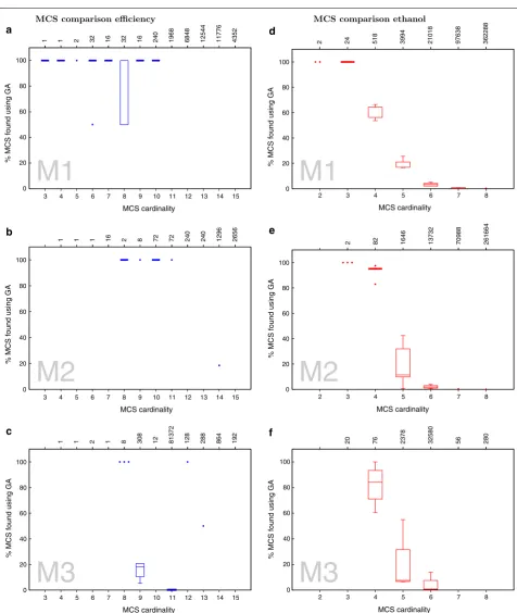
Comparing the MCSs obtained with the GA to the ones
obtained with the APM, as shown in Fig. 4a–c, reveals
that our algorithm retrieves 100 % of all low cardinality MCS. The number drops with increasing MCS’ cardi-nality. This behavior is expected as our fitness functions favors low cardinality solutions. Thus it is very unlikely that the GA will identify many high cardinality solutions. In fact, this explains the non-monotonic behavior of the line of maximum efficiency in Fig. 3c. Because the fitness function F2 allows for a trade off between cardinality and
maximum efficiency, the efficiency might decrease. Yet the fitness function still increases.
Maximizing for ethanol production
We used the fitness function F1 (Table 4) with the param-eters shown in Table 2 to maximise for ethanol yield. The GA was terminated when the fitness function remained unchanged for 15 generations.
Unlike the previous case, here our algorithm found all optimal solutions for all models. Also, we were faster than the APM in reaching the optimum for all models (see Fig. 3d–f).
Again, like in the case of maximising for efficiency, the GA retrieves 100 % of lower cardinality MCSs (Fig. 4d–f),
Table 1 The GA parameters
These parameters are used to control the running of the GA and also to get more specific results No GA parameter Description
1 t This parameter is used to specify the number of generations for which the GA will run
2 p This parameter is used to specify the number of individuals S present in one generation of the GA
3 rm This parameter is used to set the mutation rate which specifies the number of bits in an individual S that will be flipped from 0 to 1 or vice versa
4 cross This parameter is used to select among the three types of crossover operations possible here: 1point, 2point and uniform 5 elit This parameter is used to specify the fraction of the number of total individuals from the previous generation which will be
retained in the subsequent generation
6 new_S This parameter specifies the number of new individuals which will be generated in each generation, based upon information from previous generations
7 t_stop This parameter is used to set the maximum number of generations after which the GA terminates if the maximum fitness remains unchanging
8 min_1s This parameter specifies the fraction of maximum number of possible good modes which must be present in the initial popula-tion
8 wk This parameter is used by the MHSCalculator to specify the minimum number of EFMs which have to survive in given a set of desired modes D (provided as fraction of the number of EFMs in D)
and not many of the higher cardinality solutions, when compared to the solutions obtained using APM. This is a result of the fitness function, F1, which favors towards
lower cardinality MCSs. The effect of this can be observed in Fig. 3d, e where the GA first finds higher car-dinality solutions for the optimal ethanol yield and set-tles down to the lowest possible cardinality in subsequent generations.
Optimizing for a complex design
Although maximising for ethanol yield and efficiency, produces sub-optimal to optimal designs, these designs may not be the best to implement in vivo. For example, the EFMs which result in the maximum ethanol yield do not support growth. However, two of these EFMs provide maintenance energy. On the other hand, designs with
maximum efficiency do not include maximum ethanol producing EFMs. It would be preferable to have a design which combines these features. We used the fitness func-tion F3 (Table 4) with the parameters shown in Table 2 to
find optimal designs.
A similar problem was looked at in [23] where the authors optimised M1 for efficiency while ensuring that at least one of the maximal ethanol producing EFMs sur-vive in the final design. Their design included the most efficient ethanol producing EFMs as well as EFMs with maximum ethanol yield, achieved with an MCS cardi-nality of 6. A similar design was used by Trinh et al. [15] using 7 reaction knockouts. Our algorithm produces designs of similar functionality with MCSs of cardinal-ity 5, Fig. 5b. Similar results were obtained for M2, and M3 as shown in Fig. 5d and f respectively, both with MCS cardinalities of 5. Also, our algorithm was very quick in finding these designs, taking a few minutes for M1 and M2 and a few hours for M3.
Conclusion
We have presented a method for the design of minimal microbial strains of desired functionality. The designs are minimal in the sense that only a few of the total number of pathways (EFMs) are active after deletion of the pre-dicted cMCSs. Our GA uses the MHScalculator [30] to find cMCSs for a given set of desired and target EFMs. However, the optimal selection of such sets is non-intu-itive. Hence, the aim was finding the best possible set of pathways which maximise a given engineering objective.
Another GA, called the OptGene method has been previously reported which finds reaction cuts to achieve a design objective [33]. This algorithm works by testing different combinations of reaction knockouts. In con-trast, we test partitions of EFMs. Thus our search space is by orders of magnitude larger than theirs. OptGene finds many solutions too, but it cannot be guaranteed that these are minimal. Also, the knockout cardinalities are restricted to 1–10. Our approach is based on the concept of EFMs which enumerate all possible network states. OptGene however uses methods like FBA, MOMA [34], etc. to calculate the fitness which, unlike EFMs do not account for alternative pathways. Although methods which use FBA and MOMA predict optimal solutions, there is no guarantee that the predicted optimum will be achieved. In a similar vein, the method presented here has advantages over other methods which use a biased biological objective like OptKnock [35], RobustKnock [36] and tilting of the objective function [32].
Boghigian et al. [37] also use a GA and EFMs to design strains with higher product yields. Their approach however differs from the method presented START
individuals
calculate cMCS
store patterns
output results
STOP No
Yes fitnesses with highest initialise GA
create new generation
select individuals used to generate next generation generation
compute fitness & generate patterns
using stored patterns
using crossover and mutation
true
n1 + n2 + n3
high fitness in the previous
? stop =
n2
B. generate new individuals
n1
A. generate new individuals having
n3
C. take individuals
in this paper in a few major ways. First, the aim of the GA presented in [37] is to only improve product yields without considering the minimality of the knockouts.
Hence, in contrast to us their predicted knockouts are not guaranteed to be minimal. Second, the basic problems considered by both methods are different,
Complete EFMs of the network
R1 R2 R3 R4 R5 R6 R7 R8 R9 R10 R11
E1 0.0 1.0 0.0 0.25 0.0 0.5 1.0 0.0 0.25 0.5 0.0
E2 0.0 1.0 0.0 0.5 0.0 0.0 0.5 0.5 0.0 0.0 0.0
E3 0.0 0.0 1.0 0.5 0.0 1.0 1.0 0.0 0.5 1.0 0.0
E4 0.5 1.0 0.0 1.0 0.0 0.0 0.0 1.0 0.0 0.0 0.0
E5 1.0 0.0 0.0 1.0 0.0 0.0 -1.0 1.0 0.0 0.0 0.0
E6 0.0 0.0 1.0 1.0 0.0 0.0 0.0 1.0 0.0 0.0 0.0
E7 0.0 1.0 0.0 0.25 0.5 0.0 0.5 0.0 0.25 0.0 0.5
E8 0.5 1.0 0.0 0.5 1.0 0.0 0.0 0.0 0.5 0.0 1.0
E9 0.0 0.0 1.0 0.5 1.0 0.0 0.0 0.0 0.5 0.0 1.0
E10 1.0 0.0 0.0 0.5 1.0 0.0 -1.0 0.0 0.5 0.0 1.0
E11 1.0 0.0 0.0 0.5 0.0 1.0 0.0 0.0 0.5 1.0 0.0
Initial population and results
i Ei∈D Si Ci Pi YR4,i Ci F iti
1 E2,E5,E7,E11 01001010001 R2 R3 R9 00001000000 1 3 1.73 2 E4,E5,E8,E9 00011001100 R3 R7 R9 00010000000 1 3 1.73 3 E2,E3,E4,E5,E8,E9,E11 01111001101 R3 R7 00010001001 0.5 2 1.32
4 E2,E3,E4,E5,E6,E9,E11 01111100101 R9 01011100000 0.5 1 1.4
EFMs are randomly selected encoding GA individualsSisuch that a 1 & 0 indicates inclusion of the corresponding EFM inD&Trespectively.
Searching for cMCS such that at least one EFM ofDsurvives results in patternsPi.YR4,iis the least value corresponding toR4 in the surviving
EFMs.F iti=YR4,i+ 1−(Ci/n).
Creating second generation individuals
A RWSS1 crossover mutation n1 S2
01001010001
00011001100 0001100000101001011100 0010110110010011001100 0011100110001011001100 S1newS2new
B patterns00001000000 n2 00010000000
00010001001 01011100000
wt 01032101001 00011100000 S3new
C Fittest individuals01001010001 n3
00011001100 01001010001 S4new
n1 is generated by randomly selecting fromSibased onF and subjecting these to GA operations.n2 is generated by randomly selecting EFMs
based onwt, which represents survival of corresponding EFMs in the previous generations.n3 is for elitism.A,BandCcorrespond to sections
in the flowchart in Figure 1 with the same names.
Second generation and results
i Ei∈D Si Ci Pi YR4,i Ci F iti 1new E3,E4,E5,E8,E9 00111001100 R3 R7 R9 00010000000 1 3 1.73
2new E2,E4,E5,E8,E9 01011001100 R3 R9 01011000000 0.5 2 1.32
3new E4,E5,E6 00011100000 R7 R9 00010100000 1 2 1.81 4new E2,E5,E7,E11 01001010001 R2 R3 R9 00001000000 1 3 1.73
Fig. 2 GA example. Running the GA on the given toy network of 11 EFMs with the aim of maximizing production of P. The initial individuals Si and
Table 2 GA parameters for different runs
Parameters used in the various runs GA
param-eter M1 ethanol M1 effi-ciency M1 complex M2 ethanol M2 efficiency M2 complex M3 ethanol M3 efficiency M3 complex
w1 1 0 1 1 0 1 2 0 1
w2 0 50 50 0 50 50 0 10 50
w3 1 1 1 1 1 1 1 1 1
w4 1 1 1 1 1 1 1 1 1
t 100 100 100 100 100 100 100 100 100
p 50 50 50 50 50 50 50 50 50
rm 0.00025 0.00025 0.00025 0.00025 0.00025 0.00025 0.000025 0.000025 0.000025
cross 1point 1point 1point 1point 1point 1point 1point 1point 1point
elit 0.025 0.025 0.025 0.025 0.025 0.025 0.025 0.025 0.025
wk 0.03 0.017 0.04 0.025 0.01 0.03 0.01 0.0075 0.03
new_S 0.1 0.1 0.1 0.1 0.1 0.1 0.1 0.1 0.1
t_stop 15 15 15 15 15 15 15 15 15
min_1s 0.9 0.9 0.9 0.9 0.9 0.9 0.9 0.9 0.9
threads 10 10 10 10 10 10 10 10 10
Table 3 Features of models used
Features of the networks on which the GA was tested. The maximum possible values for ethanol yield, YEtoh and efficiency, ηEtoh are presented. The minimal cardinality
of MCSs which will force the network into these optimal values are also shown along with the total number of such MCSs and the number of EFMs which will survive after application of these MCSs. The corresponding fitness values, Fi have been obtained using the fitness functions presented in Table 4
Model M1 M2 M3
Model source [15] [15] [15]
Growth conditions Anaerobic, glucose + minimal media Aerobic, glucose + minimal media Aerobic, xylose, arabinose, glucose, galactose and mannose + minimal media
No: reactions 59 60 71
No: metabolites 47 49 68
Total no: EFMs 5010 38001 429275
F1 1.6170 1.6103 2.2770
maxYEtoh 0.6667 0.6667 0.6667
MCS cardinality 3 4 4
Number of MCSs 22 82 76
Number of EFMs 14 28 62
F2 7.7860 8.5283 2.3169
maxηEtoh 0.1390 0.1542 0.1542
MCS cardinality 10 13 16
Number of MCSs 240 240 2880
Number of EFMs 4 2 6
Table 4 Fitness functions used
Fitness functions used, where, w1, w2, w3 and w4 are weights associated with ethanol yield (YEtoh), ethanol efficiency (ηEtoh), MCS cardinality (|C|) and number of surviving
modes (|DC
|) respectively. These weights are used primarily to ensure desired contribution of the different variables towards the fitness function. They can also be
used to give higher preference to a particular variable. C is the MCS, n the total number of reactions and E the set of all EFMs in a network. All fitness functions were maximised
i Design objective Fitness function Fi
1 Ethanol production with minimal MCS size w1minYEtoh+w3(1− |C|/n)
2 Substrate specific productivity with minimal MCS size w2minηEtoh+w3(1− |C|/n) 3 Growth coupled product yield with minimal MCS size and maximum number of
although the final aim is the same, namely strain improvement. Boghigian et al. look for reaction knock-outs which will improve product yields. Our GA not
only maximizes the product yield but also simultane-ously searches for optimal partitions in the set of EFMs. Finally, we deal with networks where the number of
Maximizing for efficiency (F2) Maximizingforethanol(F1)
0 0.02 0.04 0.06 0.08 0.1 0.12 0.14 0.16
0 50 100 150 200 250 300 350 400 0.0 1.0 2.0 3.0 4.0 5.0 6.0 7.0 8.0 efficiency time (sec) a
M1
efficiency APM3 4 5 67 8 10 15 efficiency GA-MCS 9
10 9 11
10 fitness APM fitness GA-MCS fitness 0 0.2 0.4 0.6 0.8 1 1.2 1.4 1.6 1.8
0 50 100 150 200 250 300 350 0
0.1 0.2 0.3 0.4 0.5 0.6 0.7 0.8 ethanol time (sec) d
M1
ethanol APM2
3 4 5 6
ethanol GA-MCS 4 3 fitness APM fitness GA-MCS 0 0.02 0.04 0.06 0.08 0.1 0.12 0.14 0.16
0 1000 2000 3000 4000 5000 6000 7000 8000 9000 0.0
1.0 2.0 3.0 4.0 5.0 6.0 7.0 8.0 efficiency time (sec) b
M2
efficiency APM4 5 6 7 8 10 15 efficiency GA-MCS 9 13 12 11 10 14 fitness APM fitness GA-MCS fitness 0 0.2 0.4 0.6 0.8 1 1.2 1.4 1.6 1.8
0 500 1000 1500 2000 2500 3000 3500 4000 4500 0
0.1 0.2 0.3 0.4 0.5 0.6 0.7 0.8 ethanol time (sec) e
M2
ethanol APM3
4 5 6
ethanol GA-MCS 5 6 5 4 fitness APM fitness GA-MCS 0 0.02 0.04 0.06 0.08 0.1 0.12 0.14 0.16
10000 100000 1e+06 0.0
0.5 1.0 1.5 2.0 2.5 efficiency time (sec) c
M3
efficiency APM4
5 67 8 13 16 efficiency GA-MCS 10 14 9 14 8 fitness APM fitness GA-MCS fitness 0 0.5 1 1.5 2
100000 1e+06 0 0.1 0.2 0.3 0.4 0.5 0.6 0.7 0.8 ethanol time (sec) f
M3
ethanol APM2 3
4 8 13
ethanol GA-MCS 6
5 6 5
64
fitness APM fitness GA-MCS
MCS comparison efficiency MCS comparison ethanol
0 20 40 60 80 100
3 4 5 6 7 8 9 10 11 12 13 14 15
1 1 2 32 16 32 16 240 1968 6848 12544 11776 4352
% MCS found using GA
MCS cardinality
a
M1
0 20 40 60 80 100
2 3 4 5 6 7 8
2 24 518 3994 21018 97638 362288
% MCS found using GA
MCS cardinality d
M1
0 20 40 60 80 100
3 4 5 6 7 8 9 10 11 12 13 14 15
1 1 1 16 2 8 72 72 240 240 1296 2656
% MCS found using GA
MCS cardinality
b
M2
0 20 40 60 80 100
2 3 4 5 6 7 8
2 82 1646 13732 70988 261664
% MCS found using GA
MCS cardinality e
M2
0 20 40 60 80 100
3 4 5 6 7 8 9 10 11 12 13 14 15
1 1 2 1 8 308 12 8137
2
12
8
28
8
86
4
19
2
% MCS found using GA
MCS cardinality
c
M3
0 20 40 60 80 100
2 3 4 5 6 7 8
20 76 2378 3258
0
56 280
% MCS found using GA
MCS cardinality
f
M3
EFMs are one order of magnitude larger than that used in [37].
Tools which use EFMs to find intervention strategies
include the MHScalculator [17, 30] and a tool to
cal-culate cMCSs as part of the CellNetAnalyzer, a
MAT-LAB package providing comprehensive structural and
functional analysis of biochemical networks [38]. These methods use EFMs and hence consider the entire met-abolic landscape of the organism. The limitation of these methods is that the EFMs which must survive or be killed by an intervention have to be manually partitioned.
a
0 0.01 0.02 0.03 0.04 0.05 0.06 R_BIOt / R_GLCpts
0 0.5 1 1.5 2
R_ETOHt2r / R_GLCpts
0 0.01 0.02 0.03 0.04 0.05 0.06 0.07
R_BIOt * R_ETOHt2r / R_GLCpts
2
b
0 0.005 0.01 0.015 0.02 0.025 0.03 0.035 0.04
R_BIOt / R_GLCpts
0 0.5 1 1.5 2
R_ETOHt2r / R_GLCpts
0 0.01 0.02 0.03 0.04 0.05 0.06
R_BIOt * R_ETOHt2r / R_GLCpts
2
c
0 0.02 0.04 0.06 0.08 0.1 0.12
R_Biomass_Ecoli_core / R_GLCpts 0
0.5 1 1.5 2
R_ETOHt2r / R_GLCpts
0 0.01 0.02 0.03 0.04 0.05 0.06 0.07
R_Biomass_Ecoli_core * R_ETOHt2r / R_GLCpts
2
d
0 0.005 0.01 0.015 0.02 0.025 0.03 0.035 0.04 0.045
R_Biomass_Ecoli_core / R_GLCpts 0
0.5 1 1.5 2
R_ETOHt2r / R_GLCpts
0 0.01 0.02 0.03 0.04 0.05 0.06
R_Biomass_Ecoli_core * R_ETOHt2r / R_GLCpts
2
e
0 0.02 0.04 0.06 0.08 0.1
R_Biomass_Ecoli_core / R_norm 0
0.5 1 1.5 2
R_ETOHt2r / R_nor
m
0 0.01 0.02 0.03 0.04 0.05 0.06 0.07
R_Biomass_Ecoli_core * R_ETOHt2r / R_nor
m
2 f
0 0.005 0.01 0.015 0.02 0.025 0.03 0.035 0.04 0.045 R_Biomass_Ecoli_core / R_norm
0 0.5 1 1.5 2
R_ETOHt2r / R_nor
m
0 0.01 0.02 0.03 0.04 0.05 0.06 0.07
R_Biomass_Ecoli_core * R_ETOHt2r / R_norm
2
Fig. 5 Complex designs optimized by the GA. a, c and e show the complete set of EFMs of the M1, M2 and M3 models respectively and b, d and f represent corresponding solutions obtained using the GA which were obtained in 22, 28 min and 8 h, 48 min respectively. EFMs are represented as a function of ethanol and biomass production. Each circle represents a set of EFMs with the same yield and efficiency. The diameter of the circle
A recent method (APM [23]) overcomes this issue by calculating all partitions of EFMs for MCSs of increas-ing cardinality such that the objective is higher than that corresponding to the previous smaller MCS size. This is an exhaustive and exact method for finding intervention strategies in metabolic networks. However, this method is impractical for large networks given current compu-tational capabilities. Although the GA is not faster than the APM at very small network sizes like M1, its com-parative performance improves with increasing net-work sizes, Fig. 3. Also, when optimizing for efficiency, the GA does not reach the global optimum when APM
does, Fig. 3b, c. Note that however, an exact
compari-son to APM is not possible since APM tries to find all MCS whereas the GA tries to find the best cut set for a particular objective. Our method also incorporates the freedom to encode complex design criteria, which is not possible with the APM. Also, since the APM is based on linear programming, it is limited to linear objective functions whereas we can implement non-linear objec-tive functions as well.
An important new approach initially proposed by Ballerstein et al. [19] with further improvements in [20, 21] is able to directly find MCSs without first needing to calculate the EFMs by using the concept of hyper-graph dualisation. This gets rid of the problem of explo-sion in the number of EFMs with increasing network sizes, allowing for prediction of intervention strategies in genome-scale metabolic networks. However, these meth-ods have to specify design criteria like minimal product yield [20]. This is a limitation in that slight changes in the value of the specified design criteria may lead to different MCSs. In contrast, our algorithm tries to automatically find the best design criteria.
The GA implemented here is able to predict numer-ous good solutions to problems of product maximiza-tion which are comparable to experimentally verified designs [15]. One advantage of this method is the short time taken while dealing with bigger systems. The big-gest advantage though is the flexibility in the selection of the design criteria using the fitness function. The fitness function can be arbitrarily complex to accurately reflect the design criteria. Here it has allowed us to produce good designs without knowing the specific properties of EFMs which need to survive.
Since our approach mainly relies on a GA, it may be affected by inherent limitations of GAs, including the possibility of getting stuck at a local optimum. This may be overcome by employing multiple runs or changing the GA parameters. Note that we have considered reaction knockouts here but this can be easily translated into gene knockouts using gene-reaction associations.
Finally, we provide a brief description of the parame-ter values used. The mutation rate was set such that only two to four positions in an individual are affected, an increase in this number resulted in the GA not producing any good solutions. Decreasing this number resulted in a slower rate of improvement in fitness (data not shown). It is also possible to completely turn off mutation by set-ting rm to 0. In any case the performance of the GA can
be improved with pattern-based individual generation rather than relying solely on mutation and crossover. The number of such individuals can be adjusted with the ‘new_S’ parameter. However, too high ‘new_S’ values led to a comparatively worse GA performance (data not
shown). The parameter wk specifies the minimum
num-ber of EFMs which should survive an intervention. The lesser this value, the higher the probability of finding bet-ter solutions—because typically, optimal solutions have very few surviving EFMs, Table 3. However, small wk also
produces more solutions which in turn takes more time for pattern and fitness calculations. In order to reach the optimum with as few solutions as possible, we found that in general, wk can be large for small models (e.g., M1)
and must decrease for growing models (e.g., M2 and M3) (for exact values see Table 4). ‘min_1s’ determines the minimum number of possible good EFMs that will end up in the set of desired EFMs D in the initial population. Because the EFMs are randomly selected to be in D, not all individuals will generate viable solutions. Also, it is important that the union of Ds in the whole population nearly covers the set of good EFMs. The EFMs which are not covered must otherwise rely on mutation to be trans-ferred from T to D. The probability of this happening decreases with increasing individual size. Hence, ‘min_1s’ was set to a high value of 0.9 for all of the runs. A future direction of this work would be to study the effect of these parameters in detail. This will help get rid of the empirical setting of parameters in our GA and allow for the implementation of a protocol to automatically deter-mine these values during the running of the GA.
In summary, our algorithm is able to quickly find (near) optimal intervention strategies satisfying non-lin-ear engineering objectives in large metabolic networks. However, EFMs are still necessary for our method which is a significant bottleneck when it comes to genome-scale networks. We expect that combining the dual method [19–21], which will allow for the calculation of cMCS directly from the stoichiometric matrix, with a GA will overcome this hurdle.
Authors’ contributions
Author details
1 Department of Biotechnology, University of Natural Resources and Life
Sci-ences, Vienna, Austria. 2 Austrian Centre of Industrial Biotechnology, Vienna, Austria.
Acknowledgements
This work has been supported by the Federal Ministry of Science, Research and Economy (BMWFW), the Federal Ministry of Traffic, Innovation and Tech-nology (bmvit), the Styrian Business Promotion Agency SFG, the Standorta-gentur Tirol and ZIT - Technology Agency of the City of Vienna through the COMET-Funding Program managed by the Austrian Research Promotion Agency FFG.
Competing interests
The authors declare that they have no competing interests.
Received: 13 August 2015 Accepted: 1 December 2015
References
1. Covert MW, Schilling CH, Famili I, Edwards JS, Goryanin II, Selkov E, Palsson BO. Metabolic modeling of microbial strains in silico. Trends Biochem Sci. 2001;26(3):179–86.
2. Durot M, Bourguignon P-Y, Schachter V. Genome-scale models of bacte-rial metabolism: reconstruction and applications. FEMS Microbiol Rev. 2009;33(1):164–90.
3. Henry CS, DeJongh M, Best AA, Frybarger PM, Linsay B, Stevens RL. High-throughput generation, optimization and analysis of genome-scale metabolic models. Nat Biotechnol. 2010;28(9):977–82.
4. Thiele I, Palsson BØ. A protocol for generating a high-quality genome-scale metabolic reconstruction. Nat Protoc. 2010;5(1):93–121.
5. Oberhardt MA, Palsson BØ, Papin JA. Applications of genome-scale meta-bolic reconstructions. Mol Syst Biol. 2009;5(1):320.
6. Tenazinha N, Vinga S. A survey on methods for modeling and analyzing integrated biological networks. IEEE/ACM Trans Comput Biol Bioinform (TCBB). 2011;8(4):943–58.
7. Orth JD, Thiele I, Palsson BØ. What is flux balance analysis? Nat Biotechnol. 2010;28(3):245–8.
8. Schuster S, Hilgetag C. On elementary flux modes in biochemical reac-tion systems at steady state. J Biol Syst. 1994;2(02):165–82.
9. Schuster S, Fell DA, Dandekar T. A general definition of metabolic pathways useful for systematic organization and analysis of complex metabolic networks. Nat Biotechnol. 2000;18(3):326–32.
10. Klamt S, Stelling J. Combinatorial complexity of pathway analysis in metabolic networks. Mol Biol Rep. 2002;29(1–2):233–6.
11. Gagneur J, Klamt S. Computation of elementary modes: a unifying frame-work and the new binary approach. BMC Bioinform. 2004;5(1):175. 12. Terzer M, Stelling J. Large-scale computation of elementary flux modes
with bit pattern trees. Bioinformatics. 2008;24(19):2229–35.
13. Jungreuthmayer C, Ruckerbauer DE, Zanghellini J. regEfmtool: speeding up elementary flux mode calculation using transcriptional regulatory rules in the form of three-state logic. Biosystems. 2013;113(1):37–9. 14. David L, Bockmayr A. Computing elementary flux modes involving a
set of target reactions. IEEE/ACM Trans Comput Biol Bioinform (TCBB). 2014;11(6):1099-107.
15. Trinh CT, Unrean P, Srienc F. Minimal Escherichia coli cell for the most efficient production of ethanol from hexoses and pentoses. Appl Environ Microbiol. 2008;74(12):3634–43.
16. Hädicke O, Klamt S. Computing complex metabolic intervention strate-gies using constrained minimal cut sets. Metab Eng. 2011;13(2):204–13. 17. Jungreuthmayer C, Zanghellini J. Designing optimal cell factories: integer
programming couples elementary mode analysis with regulation. BMC Syst Biol. 2012;6(1):103.
18. Jungreuthmayer C, Nair G, Klamt S, Zanghellini J. Comparison and improvement of algorithms for computing minimal cut sets. BMC Bioin-form. 2013;14(1):318.
19. Ballerstein K, von Kamp A, Klamt S, Haus U-U. Minimal cut sets in a meta-bolic network are elementary modes in a dual network. Bioinformatics. 2012;28(3):381–7.
20. von Kamp A, Klamt S. Enumeration of smallest intervention strate-gies in genome-scale metabolic networks. PLoS Comput Biol. 2014;10(1):1003378.
21. Mahadevan R, von Kamp A, Klamt S. Genome-scale strain designs based on regulatory minimal cut sets. Bioinformatics. 2015;31(17):2844-51. 22. Jungreuthmayer C, Sonnleitner M, Striedner G, Mairhofer J, Zanghellini J.
Designing an optimally ethanol producing E. coli strain using constrained minimal cut sets. In: Proceedings of the 21st European signal processing conference; 2013.
23. Ruckerbauer D, Jungreuthmayer C, Zanghellini J. Design of optimally constructed metabolic networks of minimal functionality. PLoS One. 2014;9(3):92583.
24. Zanghellini J, Ruckerbauer DE, Hanscho M, Jungreuthmayer C. Elemen-tary flux modes in a nutshell: properties, calculation and applications. Biotechnol J. 2013;8(9):1009–16.
25. Klamt S, Gilles ED. Minimal cut sets in biochemical reaction networks. Bioinformatics. 2004;20(2):226–34.
26. Whitley D. A genetic algorithm tutorial. Stat Comput. 1994;4(2):65–85. 27. Beasley D, Martin R, Bull D. An overview of genetic algorithms: part 1.
fundamentals. Univ Comput. 1993;15:58–58.
28. Li L, Yunfei J. Computing minimal hitting sets with genetic algorithm. Technical report, DTIC Document; 2002.
29. Mitchell M. An introduction to genetic algorithms. MIT press. 1998. 30. Jungreuthmayer C, Beurton-Aimar M, Zanghellini J. Fast computation
of minimal cut sets in metabolic networks with a berge algorithm that utilizes binary bit pattern trees. IEEE/ACM Trans Comput Biol Bioinform (TCBB). 2013;10(5):1.
31. Goldberg DE, Deb K. A comparative analysis of selection schemes used in genetic algorithms. Urbana. 1991;51:61801–2996.
32. Feist AM, Zielinski DC, Orth JD, Schellenberger J, Herrgard MJ, Palsson BØ. Model-driven evaluation of the production potential for growth-coupled products of Escherichia coli. Metab Eng. 2010;12(3):173–86.
33. Patil KR, Rocha I, Förster J, Nielsen J. Evolutionary programming as a plat-form for in silico metabolic engineering. BMC Bioinplat-form. 2005;6(1):308. 34. Segre D, Vitkup D, Church GM. Analysis of optimality in natural and
perturbed metabolic networks. Proc Natl Acad Sci. 2002;99(23):15112–7. 35. Burgard AP, Pharkya P, Maranas CD. Optknock: a bilevel programming
framework for identifying gene knockout strategies for microbial strain optimization. Biotechnol Bioeng. 2003;84(6):647–57.
36. Tepper N, Shlomi T. Predicting metabolic engineering knockout strategies for chemical production: accounting for competing pathways. Bioinfor-matics. 2010;26(4):536–43.
37. Boghigian BA, Shi H, Lee K, Pfeifer BA. Utilizing elementary mode analysis, pathway thermodynamics, and a genetic algorithm for metabolic flux determination and optimal metabolic network design. BMC Syst Biol. 2010;4(1):49.
38. Klamt S, Saez-Rodriguez J, Gilles ED. Structural and functional analysis of cellular networks with cellnetanalyzer. BMC Syst Biol. 2007;1(1):2.
• We accept pre-submission inquiries
• Our selector tool helps you to find the most relevant journal • We provide round the clock customer support
• Convenient online submission • Thorough peer review
• Inclusion in PubMed and all major indexing services • Maximum visibility for your research
Submit your manuscript at www.biomedcentral.com/submit


![Fig. 3 GA performance comparison. Comparing the performance of GA-MCS against APM [23] using a single representative run for each model](https://thumb-us.123doks.com/thumbv2/123dok_us/339536.1526435/9.595.57.542.90.615/performance-comparison-comparing-performance-using-single-representative-model.webp)