RESEARCH
Fast phylogenetic inference from typing
data
João A. Carriço
1, Maxime Crochemore
2, Alexandre P. Francisco
3,4*, Solon P. Pissis
2, Bruno Ribeiro‑Gonçalves
1and Cátia Vaz
3,5Abstract
Background: Microbial typing methods are commonly used to study the relatedness of bacterial strains. Sequence‑ based typing methods are a gold standard for epidemiological surveillance due to the inherent portability of sequence and allelic profile data, fast analysis times and their capacity to create common nomenclatures for strains or clones. This led to development of several novel methods and several databases being made available for many microbial species. With the mainstream use of High Throughput Sequencing, the amount of data being accumulated in these databases is huge, storing thousands of different profiles. On the other hand, computing genetic evolution‑ ary distances among a set of typing profiles or taxa dominates the running time of many phylogenetic inference methods. It is important also to note that most of genetic evolution distance definitions rely, even if indirectly, on computing the pairwise Hamming distance among sequences or profiles.
Results: We propose here an average‑case linear‑time algorithm to compute pairwise Hamming distances among a set of taxa under a given Hamming distance threshold. This article includes both a theoretical analysis and extensive experimental results concerning the proposed algorithm. We further show how this algorithm can be successfully integrated into a well known phylogenetic inference method, and how it can be used to speedup querying local phylogenetic patterns over large typing databases.
Keywords: Computational biology, Phylogenetic inference, Hamming distance
© The Author(s) 2018. This article is distributed under the terms of the Creative Commons Attribution 4.0 International License (http://creativecommons.org/licenses/by/4.0/), which permits unrestricted use, distribution, and reproduction in any medium, provided you give appropriate credit to the original author(s) and the source, provide a link to the Creative Commons license, and indicate if changes were made. The Creative Commons Public Domain Dedication waiver (http://creativecommons.org/ publicdomain/zero/1.0/) applies to the data made available in this article, unless otherwise stated.
Background Introduction
The evolutionary relationships between different species or taxa are usually inferred through known phylogenetic analysis techniques. Some of these techniques rely on the inference of phylogenetic trees, which can be computed from DNA or Protein sequences, or from allelic profiles where the sequences of defined loci are abstracted to categorical indexes. The most popular method is Mul-tiLocus sequence typing (MLST) [1] that typically uses seven 450–700 bp fragments of housekeeping genes for a given species. Phylogenetic trees are also used in other contexts, such as to understand the evolutionary history of gene families, to allow phylogenetic foot-printing, to
trace the origin and transmission of infectious diseases, or to study the co-evolution of hosts and parasites [2, 3].
In traditional phylogenetic methods, the process of phylogenetic inference starts with a multiple alignment of the sequences under study that is then corrected using models of DNA or Protein evolution. Tree-build-ing methodologies can then be applied on the resultTree-build-ing distance matrix. These methods rely on some distance-based analysis of sequences or profiles [4].
Distance-based methods for phylogenetic analysis rely on a measure of genetic evolution distance, which is often defined directly or indirectly from the fraction of mismatches at aligned positions, with gaps either ignored or counted as mismatches. A first step of these methods is to compute this distance between all pairs of sequences. The simplest approach is to use the Hamming distance, also known as observed p-distance, defined as the number of positions at which two aligned sequences differ. Note that the Hamming distance between two
Open Access
*Correspondence: [email protected]
sequences underestimates their true evolutionary dis-tance and, thus, a correction formula based on some model of evolution is often used [2, 4]. Although dis-tance-based methods not always produce the best tree for the data, usually they also incorporate an optimality criterion into the distance model for getting more plau-sible phylogenetic reconstructions, such as the minimum evolution criterion [5], the least squares criterion [6] or the clonal complexes expansion and diversification [7]. Nevertheless, this category of methods are much faster than Maximum likelihood or Bayesian inference methods [8], making them excellent choices for the primary analy-sis of large data sets.
Most of the distance-based methods are agglomerative methods. They start with each sequence being a singleton cluster and, at each step, they join two clusters. The itera-tive process stops when all sequences are part of a single cluster, resulting in a phylogenetic tree. At each step the candidate pair is selected taking into account the distance among clusters as well as the optimality criterion chosen to adjust it.
The computation of a distance matrix (2D array con-taining the pairwise distances between the elements of a set) is a common first step for distance-based methods, such as eBURST [9], goeBURST [10], Neighbor Join-ing [11] and UPGMA [12]. This particular step dominates the running time of most methods, taking �(md2) time in general, d being the number of sequences or profiles and m the length of each sequence or profile. For large-scale datasets this running time may be quite problem-atic. And nowadays, with the mainstream use of High Throughput Sequencing, the amount of data being accu-mulated in typing databases is huge. It is common to find databases storing thousands of different profiles for a sin-gle microbial species, with each profile having thousands of loci [13, 14].
However, depending on application, on the underlying model of evolution and on the optimality criterion, it may not be strictly necessary to be aware of the complete dis-tance matrix. There are methods that continue to provide optimal solutions without a complete matrix. For such methods, one may still consider a truncated distance matrix and several heuristics, combined with final local searches through topology rearrangements, to improve the running time [6]. The goeBURST algorithm, one of our use cases in this article, is an example of a method that can work with truncated distance matrices by con-struction, i.e., one needs only to know which pairs are at Hamming distance at most k.
Our results
We propose here an average-case O(md)-time and O(md)
-space algorithm to compute the pairs of sequences,
among d sequences of length m, that are at distance at most k, when k< (m−logk−1md)·logσ, where σ is the size of the
sequences alphabet. We support our result with both a theoretical analysis and an experimental evaluation on synthetic and real datasets of different data types (MLST, cgMLST, wgMLST and SNP). We further show that our method improves goeBURST, and that we can use it to speedup querying local phylogenetic patterns over large typing databases.
A preliminary version of this paper was presented at the Workshop on Algorithms in Bioinformatics (WABI) 2017 [15].
Methods
Closest pairs in linear time
Let P be the set of profiles (or sequences) each of length m, defined over an integer alphabet , (i.e., �= {1,. . .,mO(1)}), with d= |P| and σ = |�|. Let also
H :P×P→ {0,. . .,m} be the function such that H(u, v)
is the Hamming distance between profiles u,v∈P. Given an integer threshold 0<k<m, the problem is to compute all pairs u,v∈P such that H(u,v)≤k, and the corresponding H(u, v) value, faster than the �(md2) time required to compute naïvely the complete distance matrix for the d profiles of length m.
We address this problem by indexing all profiles P using the suffix array (denoted by SA) and the longest common prefix (denoted by LCP) array [16]. We rely also on a range minimum queries (RMQ) data structure [17, 18] over the LCP array (denoted by RMQLCP). The prob-lem is then solved in three main steps:
1. Index all profiles using the SA data structure.
2. Enumerate all candidate profile pairs given the maxi-mum Hamming distance k.
3. Verify each candidate profile pair by checking if the associated Hamming distance is no more than k.
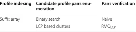
Table 1 summarizes the data structures and strategies fol-lowed in each step. Profiles are concatenated and indexed using SA. Depending on the strategy to be used, we further process the SA and build the LCP array and pre-process it for fast RMQ. This allows for enumerating candidate pro-file pairs and computing distances faster. In what follows, we detail the above steps and show how the data structures are used to improve the overall running time.
Table 1 Data structures used in our approach for each step
Profile indexing Candidate profile pairs
enu-meration Pairs verification
Step 1: Profile indexing
Profiles are concatenated and indexed in an SA in O(md)
time and space [19, 20]. Let us denote this string by s. Since we only need to compute the distances between profiles that are at Hamming distance at most k, we can conceptually split each profile into k non-overlapping blocks of length L= ⌊ m
k+1⌋ each. It is then folklore knowl-edge that if two profiles are within distance k, they must share at least one such block of length L. Our approach is based on using the SA of s to efficiently identify match-ing blocks among profile pairs. This lets us quickly filter in candidate profile pairs and filter out the ones that can never be part of the output.
Step 2: Candidate profile pairs enumeration
The candidate profile pairs enumeration step provides the pairs of profiles that do not differ in more than k posi-tions, but it may include spurious pairs. Since SA is an ordered structure, a simple solution is to use a binary search approach. For each block of each profile, we can obtain in O(Llog n) time, where n=md, all the suf-fixes that have that block as a prefix. If a given match is not aligned with the initial block, i.e., it does not occur at the same position in the respective profile, then it should be discarded. Otherwise, a candidate profile pair is reported. This searching procedure is done in O(dkLlogn)=O(nlogn) time.
Another solution relies on computing the LCP array: the longest common prefix between each pair of consec-utive elements within the SA. This information can also be computed in O(n) time and space [21]. Since SA is an
ordered structure, for the contiguous suffixes si,si+1,si+2 of s, with 0≤i<n−2, we have that the common pre-fix between si and si+1 is at least as long as the common prefix of si and si+2. By construction, it is possible to get the position of each suffix in the corresponding profile in constant time. Then, we cluster the corresponding pro-files of contiguous pairs if they have an LCP value greater than or equal to L and they are also aligned. This cluster-ing procedure can be done in O(kd2) time.
Step 3: Pairs verification
After getting the set of candidate profile pairs, a naïve solution would be to compute the distance for each pair of profiles by comparing them in linear time, i.e., O(m)
time. However, if we compute the LCP array of s, we can then perform a sequence of O(k) RMQ over the LCP
array for checking if a pair of profiles is at distance at most k. These RMQ over the LCP array correspond to longest common prefix queries between a pair of suffixes of s. Since after a linear-time pre-processing over the LCP array, RMQ can be answered in constant time per query [17], we obtain a faster approach for computing the distances. This alternative approach takes O(k) time to
verify each candidate profile pair instead of O(m) time.
Average‑case analysis
Algorithm 1 below details the solution based on LCP clusters; and Theorem 1 shows that this algorithm runs in linear time on average using linear space. We rely here on well-known results concerning the linear-time con-struction of the SA [19, 20] and the LCP array [21], as well as the linear-time pre-processing for the RMQ data structure [18].
In what follows, LCP[i], i>0, stores the length of the longest common prefix of suffixes si−1 and si of s, and RMQLCP(i,j) returns the index of the smallest element in the subarray LCP[i. . .j] in constant time [18]. We rely also on some auxiliary subroutines; let L= ⌊ m
k+1⌋:
Aligned(i) Let ℓ=i modm, i.e., the starting position
of the suffix si within a profile. Then this subroutine
returns ℓ/L if ℓ is multiple of L, and −1 otherwise.
HD( pi , pj , ℓ) Given two profiles pi and pj which share
a substring of length L, starting at index ℓL, this sub-routine computes the minimum of k and the Hamming distance between pi and pj. This subroutine relies on
RMQLCP to find matches between pi and pj and, hence,
Theorem 1 Given d profiles of length m each over an integer alphabet of size σ >1 with the letters of the
pro-files being independent and identically distributed ran-dom variables uniformly distributed over , and the max-imum Hamming distance 0<k<m, Algorithm 1 runs in O(md) average-case time and space if
Proof Let us denote by s the string of length md obtained after concatenating the d profiles. The time and space
k< (m−k−1)·logσ logmd .
required for constructing the SA and the LCP arrays for s and the RMQ data structure over the LCP array is O(md).
Let us denote by B the total number of blocks over s
and by L the block length. We set L= ⌊ m
k+1⌋ and thus we have that B=d⌊m
L⌋. Let us also denote by C a maximal set of indices over x satisfying the following:
1. The length of the longest common prefix between any two suffixes of s starting at these indices is at least L; 2. both of these suffixes start at the starting position of
a block;
Algorithm 1: Algorithm using LCP clusters.
1 Input:A setP ofdprofiles of lengthmeach; an integer threshold0< k < m.
2 Output:The setXof distinct pairs of profiles that are at Hamming distance at mostk,i.e.,
X={(u, v)∈P ×P |u < vandH(u, v)≤k}.
3 Initialization:Lets=s[0. . . n−1]be the string of lengthn=mdobtained after concatenating
thedprofiles, andL= m
k+1 . Construct the SAS fors, theLCParray forsandRMQLCP.
Initialize a hash tableHTto track verified pairs.
4 Candidate pairs enumeration:
5 X:=∅; p:=−1;Ct:=∅, for0≤t≤k
6 foreach1≤i < ndo
7 := LCP[i]
8 if ≥ Lthen
9 pi:= [i]/m
10 x:= Aligned(i)
11 if x=−1then
12 Cx:=Cx∪ {pi}
13 if p=−1then
14 pi−1:= [i−1]/m
15 x:= Aligned(i−1)
16 if x=−1then
17 Cx:=Cx∪ {pi−1}
18 p:=
19 else if p=−1then
20 Pairs enumeration:
21 foreachCt, with0≤t≤kdo
22 foreach (p, q)∈Ct×Ct:p < qdo
23 if (p, q)∈/HT then
24 HT:=HT∪ {(p, q)}
25 δ:= HD(p,q,t)
26 if δ≤kthen
27 X:=X∪ {(p, q)}
28 p:=−1;Ct:=∅, for0≤t≤k
3. and both indices correspond to the starting position of the ith block in their profiles.
This can be done in O(md) time using the LCP array
(lines 7–17). Processing all such sets C (lines 21–27) requires total time
where PROCi,j is the time required to process a pair i, j of elements of a set C, and Pairs is the sum of |C|2 over all
such sets C. We have that PROCi,j=O(k) by using RMQ over the LCP array. Additionally, by the stated assump-tion on the d profiles, the expected value for Pairs is no more than Bd
σL: we have B blocks in total and each block can only match at most d other blocks by the conditions above. Hence, the algorithm requires on average the fol-lowing running time
Let us analyze this further to obtain the relevant condi-tion on k. We have the following:
Since 0<k<m by hypothesis, we have the following:
By some simple rearrangements we have that:
Consequently, in the case when
the algorithm requires O(md) time on average. The extra
space usage is clearly O(md).
Use case 1: goeBURST algorithm
The distance matrix computation is a main step in dis-tance-based methods for phylogenetic inference. This step dominates the running time of most methods, taking �(md2) time, for d sequences of length m, since it must compute the distance among all sequence pairs. But for some methods, or when we are only interested in local phylogenies for sequences or profiles of interest, one does not need to know all pairwise distances for reconstruct-ing a phylogenetic tree. The problem addressed in this
PROCi,j×Pairs
O
md+k· Bd σL
.
k·Bd σL =
k· ⌊⌊m/(k+m 1)⌋⌋ ·d2
σ⌊km+1⌋
≤ k·
m ⌊m/(k+1)⌋
·d2
σkm+1−1
.
k·
m ⌊m/(k+1)⌋
·d2
σk+m1−1
≤ (md)
2
σk+m1−1
.
(md)2
σk+1m −1
= (md) 2 (md) logσ logmd m k+1−1 =(md)
2−(m−k−1)log(k+1)logmdσ .
k< (m−k−1)·logσ logmd
article was motivated by the goeBURST algorithm [10], our use case 1. goeBURST is one of such methods for which one must know only the pairs of sequences that are at Hamming distance at most k. The solution pro-posed here can however be extended to other distance-based phylogenetic inference methods, that rely directly or indirectly on Hamming distance computations. Note that most methods either consider the Hamming dis-tance or its correction accordingly to some formula based on some model of evolution [2, 4]. In both cases we must start by computing the Hamming distance among sequences, but not necessarily all of them [6].
The underlying model of goeBURST is as follows: a given genotype increases in frequency in the population as a consequence of a fitness advantage or of random genetic drift, becoming a founder clone in the population; and this increase is accompanied by a gradual diversification of that genotype, by mutation and recombination, forming a cluster of phylogenetic closely-related strains. This diver-sification of the “founding” genotype is reflected in the appearance of genetic profiles differing only in one house-keeping gene sequence from this genotype—single locus variants (SLVs). Further diversification of those SLVs will result in the appearance of variations of the original gen-otype with more than one difference in the allelic profile, e.g., double and triple locus variants (DLVs and TLVs).
The problem solved by goeBURST can be stated as a graphic matroid optimization problem and, hence, it follows a classic greedy approach [22]. Given the maximum Hamming distance k, we can define a graph G=(V,E), where V =P (set of profiles) and E = {(u,v)∈V2|H(u,v)≤k}. The main goal of goe-BURST is then to compute a minimum spanning forest for G taking into account the distance H and a total order on links. It starts with a forest of singleton trees (each sequence/profile is a tree). Then it constructs the optimal forest by adding links connecting profiles in different trees in increasing order accordingly to the total order, similarly to what is done in the Kruskal’s algorithm [23]. In the cur-rent implementation, a total order for links is implicitly defined based on the distance between sequences, on the number of SLVs, DLVs, TLVs, on the occurrence frequency of sequences, and on the assigned sequence identifier. With this total order, the construction of the tree consists of building a minimum spanning forest in a graph [23], where each sequence is a node and the link weights are defined by the total order. By construction, the pairs at dis-tance δ will be joined before the pairs at distance δ+1.
Use case 2: querying typing databases
length m as those in P, and k such that 0<k<m, the problem is to find all profiles v∈P such that H(u,v)≤k . One may be also interested on local phylogenetic pat-terns, but those can be inferred from found profiles using for instance the goeBURST algorithm.
Once we define the value for k, we can address this problem as follows. We index all d profiles in the data-base as before in linear time O(md), and given a query
profile u, we enumerate all candidate profiles v. We then verify as before all candidate pairs and we return only those satisfying H(u,v)≤k.
For indexing set P, we make use of the suffix tree data structure. The suffix tree T(x) of a string x is a compact trie representing all suffixes of x. It is known that the suf-fix tree of a string of length n, over an integer alphabet, can be computed in time and space O(n) [24]. For integer
alphabets, in order to access the children of an explicit node of the suffix tree by the first letter of their edge label in O(1) time, we make use of perfect hashing [25].
By using the suffix tree we find candidate matches through forward search: spelling blocks of u from the root. Specifically, given the k+1 non-overlapping blocks of length L= ⌊ m
k+1⌋ of u, we search (without reporting) for each one of them in O(L) time. Since we have k+1 blocks, it takes O(kL)=O(m) time to search for all k+1 blocks of u. Finally, we can verify and report all candidate profiles v∈P as detailed in Algorithm 2.
Although, in the worst case, Algorithm 2 runs in time
O(md+mlogmd), as we may have d matches at most,
we can prove a similar average case as in Theorem 1.
Theorem 2 Given a profile u and a set of d profiles of length m each, all over an integer alphabet of size σ >1, with the letters of the profiles being independent and identically distributed random variables uniformly distributed over , the T(s) for the string s of length md obtained after concatenating the d profiles, and the maxi-mum Hamming distance 0<k<m, Algorithm 2 runs in O(m) average-case time if
Proof Let us denote by B the total number of blocks over s and by L the block length. We set L= ⌊ m
k+1⌋ and thus we have that B=d⌊m
L⌋.
By the stated assumption on the profiles, the expected value for the number of profiles matching u is no more than B
σL: we have B blocks in total and each block can only match at most one other block in u (since they must be aligned; line 8).
k< (m−k−1)·logσ
logmd .
Moreover, since we are not relying on the LCP array in this case (profile u is not indexed), the verification step (line 12) takes O(m) time using letter comparisons.
Hence, the algorithm requires on average the following running time
Let us analyze this further to obtain the relevant condi-tion on k. We have the following:
By some simple rearrangements we have that:
Consequently, in the case when
the algorithm requires O(m) time on average.
This algorithm was implemented using a suffix array and then integrated in INNUENDO Platform, which is publicly available [24]. The INNUENDO Platform is an infrastructure that provides the required framework for data analyses from bacterial raw reads sequencing data quality insurance to the integration of epidemiological data and visualization. As such, rapid methods for classi-fication and search for closely related strains are a neces-sity for quick navigation through the platform database entries. More information about the project can be found at its website [25].
As a starting point and for the purpose of this study, a subset of 2312 wgMLST profiles of Escherichia coli retrieved from Enterobase [13] were included in the INNUENDO database as well as their ancillary data and predefined core-genome cluster classification. Two tab-separated files containing the wgMLST and cgMLST profiles for the E. coli strains were also created to allow storing information on the currently available profiles and for updating with profiles that will become available upon the platform analyses.
One of two index files are used depending on the type of search we want to perform: classification or search for k-closest. The cgMLST index file is used for strain classi-fication, which relies on a nomenclature designed for the cgMLST profiles. As such, and since a pre-classification
O(m+m· B
σL).
m· B
σL =
m· ⌊⌊m/(mk+1)⌋⌋ ·d
σ⌊ m k+1⌋
≤
m·(⌊m/(mk+1)⌋)·d
σ m k+1−1
≤ m 2d
σ m k+1−1
.
m2d
σkm+1−1
= m
2d
(md) logσ logmd(
m k+1−1)
=m(md)1−
(m−k−1)logσ (k+1)logmd .
k< (m−k−1)·logσ
logmd
was performed on the database of E. coli strains, we con-tinued using it for comparison purposes. However, when searching for the k-closest profiles, we take into consid-eration all targets available in the wgMLST profiles using the wgMLST index file for a higher discriminatory power.
Each time a new profile is generated from the platform, it requires classification. The INNUENDO Platform performs the classification step based on the approach described in our "Use case 2: querying typing databases" with a given maximum of k differences over core genes. It uses the cgMLST index file for the search since the classification is constructed based on those number of loci. If the method returns at least one match, it classi-fies the new profile with the classification of the closest. If not, a new classification is assigned. A new entry is then added to the INNUENDO database as well as to the cgMLST and wgMLST profiles files and the index files are updated.
In the case of the search for the k-closest, it is useful to define the input data for visualization methods accord-ing to a defined number of differences on close strains. For each profile used as input for the search, the method searches for the k-closest strains considering at most k differences among all wgMLST loci. Since duplicate matches can occur between the profiles used for each search, the final file used as input for the visualization methods is the intersection of the results of the k-closest profiles between each input strain. The set of strain iden-tifiers are then used to query the INNUENDO database to get the profiles and ancillary data to be sent to PHY-LOViZ Online [26] for further analysis, namely with the goeBURST algorithm.
The drawback of using this method for classification and search is the need for rebuilding the index each time there is a new profile, which will depend on the number of profile entries on the database. Nevertheless, the num-ber of updates is rather smaller compared to the numnum-ber of queries and the index can be build in the background, with search functionalities still using the old index during the process. In our implementation, the index and related data structures are serialized in secondary memory and they are accessed by mapping them into memory. The implementation of the underlying tool is made publicly available [27].
Experimental evaluation
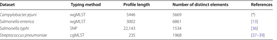
We evaluated the proposed approach to compute the pairs of profiles at distance at most k using both real and synthetic datasets. We used real datasets obtained through different typing schemas, namely whole-genome multi-locus sequence typing (wgMLST) data, core-genome multi-locus sequence typing (cgMLST) data, and single-nucleotide polymorphism (SNP) data. Table 2 summarizes the real datasets used. We should note that wgMLST and cgMLST datasets contain sequences of integers, where each column corresponds to a locus and different values in the same column denote differ-ent alleles. Synthetic datasets comprise sets of binary sequences of variable length, uniformly sampled, allow-ing us to validate our theoretical findallow-ings.
We implemented both versions described above in the C programming language: one based on binary search over the SA; and another one based on find-ing clusters in the LCP array. Since allelic profiles can be either string of letters or sequences of integers, we relied on libdivsufsort library [28] and qsuf-sort code [29, 30], respectively. For RMQ over the LCP array, we implemented a fast well-known solution that uses constant time per query and linearithmic space for pre-processing [17].
All tests were conducted on a machine running Linux, with an Intel(R) Xeon(R) CPU E5-2630 v3 @ 2.40 GHz (8 cores, cache 32 KB/4096 KB) and with 32 GB of RAM. All binaries where produced using GCC 5.3 with full optimization enabled.
Synthetic datasets
We first present results with synthetic data for different values of d, m and k. All synthetic sequences are binary sequences uniformly sampled. Results presented in this section were averaged over ten runs and for five different sets of synthetic data.
The bound proved in Theorem 1 was verified in prac-tice. For k satisfying the conditions in Theorem 1, the running time of our implementation grows almost line-arly with n, the size of the input. We can observe in Fig. 1 a growth slightly above linear. Since we included the time for constructing the SA, the LCP array and the RMQ data
structure, with the last one in linearithmic time, that was expected.
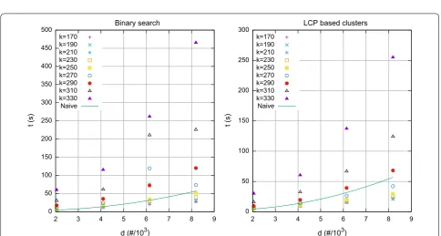
We also tested our method for values of k exceeding the bound shown in Theorem 1. For d=m=4096 and a binary alphabet, the bound for k given in Theorem 1 is no more than ⌊m/(2 logm)⌋ =170. For k above this bound we expect that proposed approaches are no longer com-petitive with the naïve approach. As shown in Fig. 2, for k>250 and k>270 respectively, both limits above the predicted bound, the running time for both computing pairwise distances by finding lower and higher bounds in the SA, and by processing LCP based clusters, becomes slower than the running time of the naïve approach.
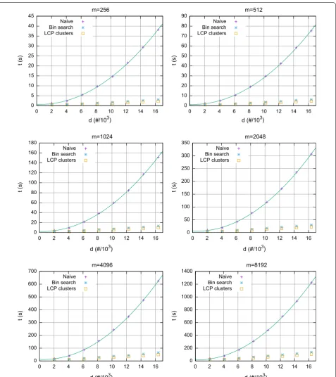
In Fig. 3 we have the running time as a function of the number d of profiles, for different values of m and for k satisfying the bound given in Theorem 1. The running time for the naïve approach grows quadratically with d, while it grows linearly for both computing pairwise dis-tances by finding lower and higher bounds in the SA, and by processing LCP based clusters. Hence, for synthetic data, as described by Theorem 1, the result holds.
Real datasets
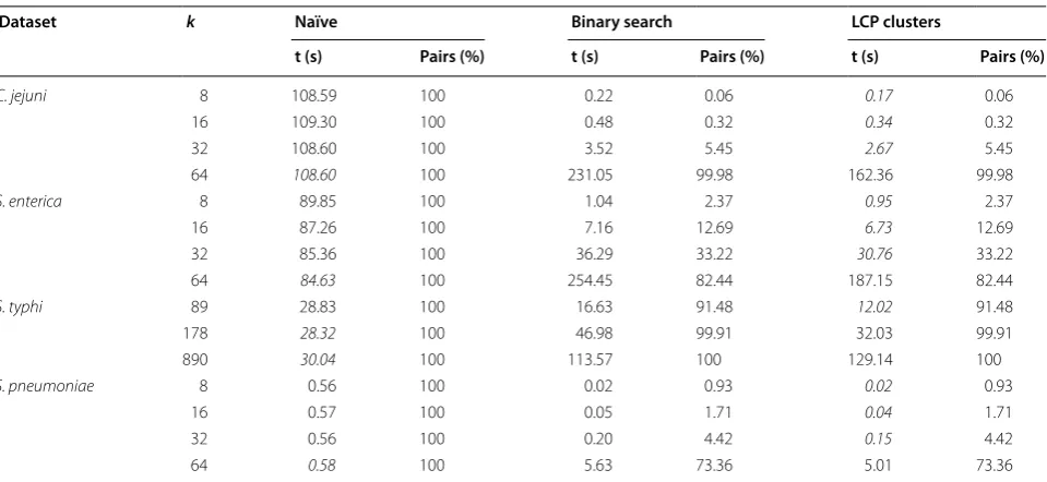
For each dataset in Table 2, we ranged the threshold k accordingly and compared the approaches discussed in "Methods" section with the naïve approach that com-putes the distance for all sequence pairs. Results are pro-vided in Table 3.
In most cases, the approach based on the LCP clusters is the fastest up to two orders of magnitude compared to the naïve approach. As expected, in the case when data are not uniformly random, our method works reasonably well for smaller values of k than the ones implied by the bound in Theorem 1. As an example, the upper bound on k for C. jejuni would be around 200, but the running time for the naïve approach is already better for k=64. We should note however that the number of candidate profile pairs at Hamming distance at most k is much higher than the expected number when data are uniformly random. This tells us that we can design a simple hybrid scheme that chooses a strategy (naïve or the proposed method) depending on the nature of the input data. It seems also to point out clustering effects on profile dissimilarities,
Table 2 Real datasets used in the experimental evaluation
(*) Dataset provided by the Molecular Microbiology and Infection Unit, IMM
Dataset Typing method Profile length Number of distinct elements References
Campylobacter jejuni wgMLST 5446 5669 (*)
Salmonella enterica wgMLST 3002 6861 [13]
Salmonella typhi SNP 22,143 1534 [36]
0 20 40 60 80 100 120 140
0 20 40 60 80 100 120 140
t (s)
n = d*m (#/106) Binary search
0 20 40 60 80 100 120
0 20 40 60 80 100 120 140
t (s)
n = d*m (#/106) LCP based clusters
Fig. 1 Synthetic datasets, with σ=2 and k= ⌊m/(2 logm)⌋ according to Theorem 1. Running time for computing pairwise distances by finding lower and higher bounds in the SA, and by processing LCP based clusters, as function of the input size n=dm
0 50 100 150 200 250 300 350 400 450 500
2 3 4 5 6 7 8 9
t (s)
d (#/103) Binary search
k=170 k=190 k=210 k=230 k=250 k=270 k=290 k=310 k=330 Naive
0 50 100 150 200 250 300
2 3 4 5 6 7 8 9
t (s)
d (#/103) LCP based clusters
k=170 k=190 k=210 k=230 k=250 k=270 k=290 k=310 k=330 Naive
0 5 10 15 20 25 30 35 40 45
0 2 4 6 8 10 12 14 16
t (s)
d (#/103) m=256
Naive Bin search LCP clusters
0 10 20 30 40 50 60 70 80 90
0 2 4 6 8 10 12 14 16
t (s)
d (#/103) m=512
Naive Bin search LCP clusters
0 20 40 60 80 100 120 140 160 180
0 2 4 6 8 10 12 14 16
t (s
)
d (#/103) m=1024
Naive Bin search LCP clusters
0 50 100 150 200 250 300 350
0 2 4 6 8 10 12 14 16
t (s
)
d (#/103) m=2048
Naive Bin search LCP clusters
0 100 200 300 400 500 600 700
0 2 4 6 8 10 12 14 16
t (s)
d (#/103) m=4096
Naive Bin search LCP clusters
0 200 400 600 800 1000 1200 1400
0 2 4 6 8 10 12 14 16
t (s)
d (#/103) m=8192
Naive Bin search LCP clusters
Fig. 3 Synthetic datasets, with σ=2 and k= ⌊m/(2 logm)⌋ according to Theorem 1. Running time for computing pairwise distances naïvely, by
which we may exploit to improve our results. We leave both tasks as future work for the full version of this article.
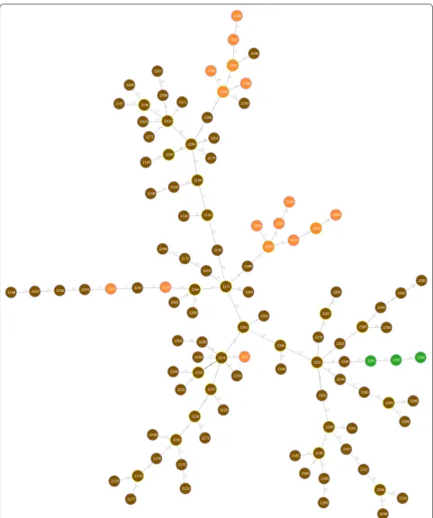
We incorporated the approach based on finding lower and higher bounds in the SA in the implementation of goeBURST algorithm, discussed in "Methods" section. We did not incorporate the approach based on the LCP clusters as the running time did not improve much as observed above. Since running times are similar to those reported in Table 3, we discuss only the running time for C. jejuni. We need only to index the input once. We can then use the index in the different stages of the algo-rithm and for different values of k. In the particular case of goeBURST, we use the index twice: once for comput-ing the number of neighbors at a given distance, used for untying links according to the total order discussed in the description of goeBURST algorithm in methods section, and a second time for enumerating pairs at dis-tance below a given threshold. Note that the goeBURST algorithm does not aim to link all nodes, but to identify clonal complexes (or connected components) for a given threshold on the distance among profiles [10]. In the case of C. jejuni dataset, and for k =52, the running time is around 36 s, while the naïve approach takes around 115 s, yielding a threefold speedup. In this case we get sev-eral connected components, i.e., sevsev-eral trees, connect-ing the most similar profiles. We provide the tree for the largest component in Fig. 4, where each node represents a profile. The nodes are colored according to one of the loci for which profiles in this cluster differ. Note that this tree is optimal with respect to the criterion used by the
goeBURST algorithm, not being affected by the threshold on the distance. In fact, since this problem is a graphic matroid, the trees found for a given threshold will be always subtrees of the trees found for larger thresh-olds [22]. Comparing this tree with other inference meth-ods is beyond the scope of this article; the focus here was on the faster computation of an optimal tree under this model.
In many studies, the computation of trees based on pairwise distances below a given threshold, usually small compared with the total number of loci, combined with ancillary data, such as antibiotic resistance and host information, allows microbiologists to uncover evolution patterns and study the mechanisms underlying the trans-mission of infectious diseases [31].
Conclusions
Most distance-based phylogenetic inference methods rely directly or indirectly on Hamming distance compu-tations. The computation of a distance matrix is a com-mon first step for such methods, taking �(md2) time in general, with d being the number of sequences or profiles and m the length of each sequence or profile. For large-scale datasets this running time may be problematic; however, for some methods, we can avoid to compute all-pairs distances [6].
We addressed this problem when only a truncated dis-tance matrix is needed, i.e., one needs to know only which pairs are at Hamming distance at most k. This problem was motivated by the goeBURST algorithm [10], which relies on a truncated distance matrix by construction. Table 3 Time and percentage of pairs processed for each method and dataset
The minimum time for each row is highlighted in italic
Dataset k Naïve Binary search LCP clusters
t (s) Pairs (%) t (s) Pairs (%) t (s) Pairs (%)
C. jejuni 8 108.59 100 0.22 0.06 0.17 0.06
16 109.30 100 0.48 0.32 0.34 0.32
32 108.60 100 3.52 5.45 2.67 5.45
64 108.60 100 231.05 99.98 162.36 99.98
S. enterica 8 89.85 100 1.04 2.37 0.95 2.37
16 87.26 100 7.16 12.69 6.73 12.69
32 85.36 100 36.29 33.22 30.76 33.22
64 84.63 100 254.45 82.44 187.15 82.44
S. typhi 89 28.83 100 16.63 91.48 12.02 91.48
178 28.32 100 46.98 99.91 32.03 99.91
890 30.04 100 113.57 100 129.14 100
S. pneumoniae 8 0.56 100 0.02 0.93 0.02 0.93
16 0.57 100 0.05 1.71 0.04 1.71
32 0.56 100 0.20 4.42 0.15 4.42
Both the problem and techniques discussed here are related to average-case approximate string matching [32, 33]. We proposed here an average-case linear-time and linear-space algorithm to compute the pairs of sequences or profiles that are at Hamming distance at most k, when k< (m−logk−1md)·logσ, where σ is the size of the alphabet. We
integrated our solution in goeBURST demonstrating its effectiveness using both real and synthetic datasets.
We must note however that our analysis holds for uni-formly random sequences and, hence, as observed with real data, the presented bound may be optimistic. It is thus interesting to investigate how to address this prob-lem taking into account local conserved regions within sequences. Moreover, it might be interesting to consider in the analysis null models such as those used to evalu-ate the accuracy of distance-based phylogenetic inference methods [4].
The proposed approach is particularly useful when one is interested in local phylogenies, i.e., local patterns of evolution, such as searching for similar sequences or pro-files in large typing databases, as in our "Use case 2: que-rying typing databases". In this case we do not need to construct full phylogenetic trees, with tens of thousands of taxa. We can focus our search on the most similar sequences or profiles, within a given threshold k. There are however some issues to be solved in this scenario, namely, dynamic updating of the data structures used in our algorithm. Note that after querying a database, if new sequences or profiles are identified, then we should be able to add them while keeping our data structures updated. Although more complex and dynamic data structures are known, a technique proposed recently for adding dynamism to otherwise static data structures can be useful to address this issue [34]. This and other chal-lenges raised above are left as future work.
Authors’ contributions
MC, APF, SPP and CV conceived the study and contributed for the design and analysis of the methods and experimental evaluation. APF, SPP and CV imple‑ mented Algorithm 1 and run the experiments. JAC conceived the case study 2 and contributed with the biological background. APF and BRG implemented Algorithm 2 and integrated it in INNUENDO Platform. All authors contributed to the writing of the manuscript. All authors read and approved the final manuscript.
Author details
1 Faculdade de Medicina, Instituto de Microbiologia and Instituto de Medicina Molecular, Universidade de Lisboa, Lisboa, Portugal. 2 Department of Informat‑ ics, King’s College London, London, UK. 3 INESC‑ID Lisboa, Rua Alves Redol 9, 1000‑029 Lisboa, Portugal. 4 Instituto Superior Técnico, Universidade de Lisboa, Lisboa, Portugal. 5 Instituto Superior de Engenharia de Lisboa, Instituto Politécnico de Lisboa, Lisboa, Portugal.
Acknowledgements
This work was partly supported by the Royal Society International Exchanges Scheme, and by the following projects: BacGenTrack (TUBITAK/0004/2014) funded by FCT (Fundação para a Ciência e a Tecnologia) / Scientific and Technological Research Council of Turkey (Türkiye Bilimsel ve Teknolojik Araşrrma Kurumu, TÜBİTAK), PRECISE (LISBOA‑01‑0145‑FEDER‑016394)
and ONEIDA (LISBOA‑01‑0145‑FEDER‑016417) projects co‑funded by FEEI (Fundos Europeus Estruturais e de Investimento) from “Programa Operacional Regional Lisboa 2020” and by national funds from FCT, UID/CEC/500021/2013 funded by national funds from FCT, and INNUENDO project [25] co‑funded by the European Food Safety Authority (EFSA), grant agreement GP/EFSA/ AFSCO/2015/01/CT2 (“New approaches in identifying and characterizing microbial and chemical hazards”). The conclusions, findings, and opinions expressed in this review paper reflect only the view of the authors and not the official position of the European Food Safety Authority (EFSA).
Competing interests
The authors declare that they have no competing interests.
Publisher’s Note
Springer Nature remains neutral with regard to jurisdictional claims in pub‑ lished maps and institutional affiliations.
Received: 31 October 2017 Accepted: 22 December 2017
References
1. Maiden MC, Bygraves JA, Feil EJ, Morelli G, Russell JE, Urwin R, Zhang Q, Zhou J, Zurth K, Caugant DA, Feavers IM, Achtman M, Spratt BG. Multilo‑ cus sequence typing: a portable approach to the identification of clones within populations of pathogenic microorganisms. Proc Natl Acad Sci USA. 1998;95(6):3140–5.
2. Huson DH, Rupp R, Scornavacca C. Phylogenetic networks: concepts, algorithms and applications. New York: Cambridge University Press; 2010. https://doi.org/10.1017/CBO9780511974076.
3. Robinson DA, Feil EJ. Bacterial population genetics in infectious disease. Hoboken: Wiley; 2010. https://doi.org/10.1002/9780470600122. 4. Saitou N. Introduction to evolutionary genomics. London: Springer; 2013.
https://doi.org/10.1007/978‑1‑4471‑5304‑7.
5. Desper R, Gascuel O. Fast and accurate phylogeny reconstruction algorithms based on the minimum‑evolution principle. J Comput Biol. 2002;9(5):687–705. https://doi.org/10.1089/106652702761034136. 6. Pardi F, Gascuel O. Distance‑based methods in phylogenetics. In: Encyclo‑
pedia of evolutionary biology. Oxford: Elsevier; 2016. p. 458–65. https:// doi.org/10.1016/B978‑0‑12‑800049‑6.00206‑7.
7. Feil EJ, Holmes EC, Bessen DE, Chan M‑S, Day NP, Enright MC, Goldstein R, Hood DW, Kalia A, Moore CE, et al. Recombination within natural popula‑ tions of pathogenic bacteria: short‑term empirical estimates and long‑ term phylogenetic consequences. Proc Natl Acad Sci. 2001;98(1):182–7. https://doi.org/10.1073/pnas.98.1.182.
8. Yang Z, Rannala B. Molecular phylogenetics: principles and practice. Nat Rev Genet. 2012;13(5):303–14.
9. Feil EJ, Li BC, Aanensen DM, Hanage WP, Spratt BG. eBURST: inferring patterns of evolutionary descent among clusters of related bacte‑ rial genotypes from multilocus sequence typing data. J Bacteriol. 2004;186(5):1518–30. https://doi.org/10.1128/JB.186.5.1518‑1530.2004. 10. Francisco AP, Bugalho M, Ramirez M. Global optimal eBURST analysis of multilocus typing data using a graphic matroid approach. BMC Bioin‑ form. 2009;10(1):152. https://doi.org/10.1186/1471‑2105‑10‑152. 11. Saitou N, Nei M. The neighbor‑joining method: a new method for recon‑
structing phylogenetic trees. Mol Biol Evol. 1987;4(4):406–25. https://doi. org/10.1093/oxfordjournals.molbev.a040454.
12. Sokal RR. A statistical method for evaluating systematic relationships. Univ Kans Sci Bull. 1958;38:1409–38.
13. Sergean M, Zhou Z, Alikhan NF, Achtman M. EnteroBase. https://enter‑ obase.warwick.ac.uk/. Accessed 31 Oct 2017.
14. Jolley KA, Maiden MCJ. BIGSdb: scalable analysis of bacterial genome variation at the population level. BMC Bioinform. 2010;11:595.
• We accept pre-submission inquiries
• Our selector tool helps you to find the most relevant journal • We provide round the clock customer support
• Convenient online submission • Thorough peer review
• Inclusion in PubMed and all major indexing services • Maximum visibility for your research
Submit your manuscript at www.biomedcentral.com/submit
Submit your next manuscript to BioMed Central
and we will help you at every step:
Germany. 2017. https://doi.org/10.4230/LIPIcs.WABI.2017.9. http://drops. dagstuhl.de/opus/volltexte/2017/7652.
16. Manber U, Myers G. Suffix arrays: a new method for on‑line string searches. SIAM J Comput. 1993;22(5):935–48. https://doi. org/10.1137/0222058.
17. Bender MA, Farach‑Colton M. The LCA problem revisited. In: LATIN 2000: theoretical informatics: 4th Latin American symposium. Lecture notes in computer Sscience, vol. 1776, p. 88–94. Springer, Berlin, Heidelberg. 2000. https://doi.org/10.1007/10719839_9.
18. Bender MA, Farach‑Colton M, Pemmasani G, Skiena S, Sumazin P. Lowest common ancestors in trees and directed acyclic graphs. J Algorithms. 2005;57(2):75–94. https://doi.org/10.1016/j.jalgor.2005.08.001.
19. Kärkkäinen J, Sanders P, Burkhardt S. Linear work suffix array construction. J ACM. 2006;53(6):918–36. https://doi.org/10.1145/1217856.1217858. 20. Ko P, Aluru S. Space efficient linear time construction of suffix arrays. In:
Annual symposium on combinatorial pattern matching. Lecture notes in computer science, vol. 2676, p. 200–10. Springer, Berlin, Heidelberg. 2003. https://doi.org/10.1016/j.jda.2004.08.002.
21. Kasai T, Lee G, Arimura H, Arikawa S, Park K. Linear‑time longest‑common‑ prefix computation in suffix arrays and its applications. In: Annual sym‑ posium on combinatorial pattern matching. Springer. 2001. p. 181–92. https://doi.org/10.1007/3‑540‑48194‑X.
22. Papadimitriou CH, Steiglitz K. Combinatorial optimization: algorithms and complexity. Upper Saddle River: Prentice‑Hall Inc; 1982.
23. Kruskal JB. On the shortest spanning subtree of a graph and the traveling salesman problem. Proc Am Math Soc. 1956;7(1):48–50. https://doi. org/10.2307/2033241.
24. B‑UMMI: INNUENDO platform. https://github.com/B‑UMMI/INNUENDO. Accessed 31 Oct 2017.
25. INNUENDO: a novel cross‑sectorial platform for the integration of genom‑ ics in surveillance of foodborne pathogens. http://www.innuendoweb. org/. Accessed 31 Oct 2017.
26. Ribeiro‑Gonçalves B, Francisco AP, Vaz C, Ramirez M, Carriço JA. PHY‑ LOViZ online: web‑based tool for visualization, phylogenetic inference, analysis and sharing of minimum spanning trees. Nucleic Acids Res. 2016;44(Webserver–Issue):246–51. https://doi.org/10.1093/nar/gkw359. 27. B‑UMMI: fast MLST searching and querying. https://github.com/B‑UMMI/
fast‑mlst. Accessed 31 Oct 2017.
28. Mori Y. A lightweight suffix‑sorting library. https://github.com/y‑256/ libdivsufsort. Accessed 31 Oct 2017.
29. Larsson NJ, Sadakane K. Suffix sorting implementation to accompany the paper Faster Suffix Sorting. http://www.larsson.dogma.net/qsufsort.c. Accessed 31 Oct 2017.
30. Larsson NJ, Sadakane K. Faster suffix sorting. Theor Comput Sci. 2007;387(3):258–72. https://doi.org/10.1016/j.tcs.2007.07.017. 31. Francisco AP, Vaz C, Monteiro PT, Melo‑Cristino J, Ramirez M, Carriço JA.
PHYLOViZ: phylogenetic inference and data visualization for sequence based typing methods. BMC Bioinform. 2012;13(1):87. https://doi. org/10.1186/1471‑2105‑13‑87.
32. Fredriksson K. Average‑optimal single and multiple approximate string matching. ACM J Exp Algorithm. 2004;9:1–4. https://doi. org/10.1145/1005813.1041513.
33. Barton C, Iliopoulos CS, Pissis SP. Fast algorithms for approximate circular string matching. Algorithms Mol Biol. 2014;9:9. https://doi. org/10.1186/1748‑7188‑9‑9.
34. Munro JI, Nekrich Y, Vitter JS. Dynamic data structures for document collections and graphs. In: Proceedings of the 34th ACM symposium on principles of database systems. ACM, New York, NY, USA. 2015. https:// doi.org/10.1145/2745754.2745778.
35. Nascimento M, Sousa A, Ramirez M, Francisco AP, Carriço JA, Vaz C. PHY‑ LOViZ 2.0: providing scalable data integration and visualization for mul‑ tiple phylogenetic inference methods. Bioinformatics. 2017;33(1):128–9. https://doi.org/10.1093/bioinformatics/btw582.
36. Page AJ, Taylor B, Delaney AJ, Soares J, Seemann T, Keane JA, Harris SR. SNP‑sites: rapid efficient extraction of SNPs from multi‑FASTA align‑ ments. Microbial Genom. 2016;2(4):e000056. https://doi.org/10.1099/ mgen.0.000056.
37. Croucher NJ, Finkelstein JA, Pelton SI, Mitchell PK, Lee GM, Parkhill J, Bentley SD, Hanage WP, Lipsitch M. Population genomics of post‑vaccine changes in pneumococcal epidemiology. Nat Genet. 2013;45(6):656–63. https://doi.org/10.1038/ng.2625.
38. Chewapreecha C, Harris SR, Croucher NJ, Turner C, Marttinen P, Cheng L, Pessia A, Aanensen DM, Mather AE, Page AJ, Salter SJ, Harris D, Nosten F, Goldblatt D, Corander J, Parkhill J, Turner P, Bentley SD. Dense genomic sampling identifies highways of pneumococcal recombination. Nat Genet. 2014;46(3):305–9. https://doi.org/10.1038/ng.2895.