Uncertainty analysis using Bayesian Model Averaging: a case study of input variables to energy models and inference to associated uncertainties of energy scenarios

(1)

O R I G I N A L A R T I C L E

Open Access

Uncertainty analysis using Bayesian Model

Averaging: a case study of input variables

to energy models and inference to

associated uncertainties of energy

scenarios

Monika Culka

Abstract

Background:Energy models are used to illustrate, calculate and evaluate energy futures under given assumptions. The results of energy models are energy scenarios representing uncertain energy futures.

Methods:The discussed approach for uncertainty quantification and evaluation is based on Bayesian Model Averaging for input variables to quantitative energy models. If the premise is accepted that the energy model results cannot be less uncertain than the input to energy models, the proposed approach provides a lower bound of associated uncertainty. The evaluation of model-based energy scenario uncertainty in terms of input variable uncertainty departing from a probabilistic assessment is discussed.

Results:The result is an explicit uncertainty quantification for input variables of energy models based on well-established measure and probability theory. The quantification of uncertainty helps assessing the predictive potential of energy scenarios used and allows an evaluation of possible consequences as promoted by energy scenarios in a highly uncertain economic, environmental, political and social target system.

Conclusions:If societal decisions are vested in computed model results, it is meaningful to accompany these with an uncertainty assessment. Bayesian Model Averaging (BMA) for input variables of energy models could add to the currently limited tools for uncertainty assessment of model-based energy scenarios.

Keywords:Uncertainty assessment, Bayesian model averaging, Energy model, Probability

JEL:C520, C32

Background

In this paper, a method for an explicit, quantitative un-certainty assessment suitable for quantitative energy models with input variables is proposed. The method discussed renders the uncertainty evaluation more tan-gible to modellers and receivers of energy model scenar-ios. It can be perceived as an application of the discussion provided by Culka in [1]. The proposed quanti-fication of uncertainty departs from a probabilistic assess-ment in Bayesian terms. The Bayesian Model Averaging

(BMA) method is a well-established concept which already has been applied in energy economics [2, 3]. By intention, the method presented is not novel and relies on accepted concepts and theories. However, the presented definition of uncertainty derived from basic probability theory is novel, and the application was not formulated as such for energy economic contexts to my knowledge. The approach could add to the currently limited tools of un-certainty quantification in energy modelling. The pre-sented method as discussed in this paper, does not claim to resolve the question of reliability of model results. In particular, it is limited to the assessment of input variables, and a specific kind of assumption uncertainty. It does Correspondence:monika.culka@nica-research.net

NICA The Research Initiative, Dekan Hintner Str. 10, 6330 Kufstein, Austria

(2)

explicitly not address the quantification of model-specific error propagation.

The objectives of this paper are to (1) raise awareness that uncertainty in energy scenarios needs to be ad-dressed (“Background”section ), (2) provide a definition of an uncertainty measure (“Methods” section) and (3) exemplify the uncertainty assessment for input variables with BMA and probabilistic uncertainty in a case study (Methods: “Case study” section). In this section, I will focus on the relevance of such a method based on current practice and criticisms on available uncertainty assessments. I am briefly introducing the kinds of uncer-tainty the case study assess, and I am ending the section with the introduction of the premise which has to be ac-cepted in order to formulate an uncertainty assessment for the results of energy models based on their input variables.

Energy models are representations of the energy sys-tem including different sub-syssys-tems. The target syssys-tem cannot be described solely in terms of one system with-out ignoring decisive elements. In contrast, a system model of a physical process could be described for ex-ample by the laws of thermodynamics. Energy models, however, represent a target system involving physical, societal, political, environmental and other aspects as central elements, for example, energy system models such as TIMES [4], or MESSAGE [5]. Many energy models aim at a broad inclusion of target system ele-ments, e.g. an inclusion of different energy carriers, dif-ferent economic sectors, environmental aspects and extensive regional inclusion. The results are large and complex models that are difficult to analyse with respect to uncertainty and internal error propagation. Error propagation estimation and analysis of individual models may even be impossible due to the complexity of math-ematical formulations, ad hoc assumptions, idealisa-tions of the target system and lack of empirical verification (of parts) of the model. The choice of model boundaries, the level of abstraction or idealisa-tion, mathematical representation and used optimisa-tion routines are highly individual for every energy model. Early attempts of quality improvement for en-ergy models have mainly focussed on technical model-ling aspects [6]. Recent evaluation processes include next to classical uncertainty estimation methods [7] also approaches for developing adaptive policies under uncertainty [8]. Classical uncertainty estimation in-cludes statistical analysis as, for example, output means, variances, sampling techniques, e.g. Monte Carlo, sensitivity analysis, and the like. In the light of uncertainty, which is not uniquely due to model char-acteristics, other techniques as robustness analysis or explicit integration of subjective features have been dis-cussed recently [9]. These methods are fodis-cussed on

decision support, which is especially relevant if energy model results are used to derive recommendations.

Models are used to compute scenarios of the energy system in future. These may be demanded by economy, political institutions or stakeholders. Assisting the evalu-ation of impacts for policy analysis is a central role of quantitative energy modelling [10, 11]. Mathematical en-ergy models are a simplified and idealised representation of a target system. Due to these simplifications and idea-lisations of mathematical models, the uncertainty re-garding assumptions and stochastic processes in (parts of ) the energy system being modelled, energy models and their results—energy scenarios—face uncertainty. As energy scenarios can serve for political advice and may be influential for political decisions, an uncertainty ana-lysis for energy scenarios seems to be necessary. For the decision maker, it would provide relevant information regarding the relevance and reliability of energy scenarios.

What the term “scenario” refers to is not clearly de-fined in the literature. Van Notten describes more than 11 definitions and common applications for scenarios [12]. Lindgren concisely summarises paradoxes and ap-plications for scenario techniques [13]. Both agree that scenario building is a fundamentally intuitive and cre-ative process, involving associations, inferred causal pat-terns and other ideas. Scenarios are a widely used technique if future developments are to be evaluated [14]. Önkal et al. differentiate between method-based statistical forecasting and forecasting with scenarios and emphasise the latter being a conceptual description of a plausible future which underlines reasoning and uncer-tainty [15]. In this paper, the term energy scenario refers to the output of quantitative energy models of any math-ematical kind. In energy economics, energy scenarios are used to describe possible, plausible or probable future energy system states [16]. The limitation of the future to some defined input scenarios, also called storylines or key assumptions, implies a subjective and decisive pre-selection of futures scrutinised with an energy model. This is a delicate process which should involve expert knowledge and rigorous attention concerning plausibility and reciprocal assumption impact [17]. The agreed as-sumptions, model design and formulation, and the spe-cific question to be answered by an energy model, form the basis for the calculation of energy scenarios. So, en-ergy scenarios should be understood for this paper as the quantitative and interpretative outputs of mathemat-ical energy models.

(3)

2030 is energy scenario X”. Attention should be paid to the disclaimer "if the assumptions hold". This makes any energy scenario (the output of a given energy model) con-ditional on the input assumptions. Many model-based outlooks explicitly avoid terms like “forecast” being well aware that energy scenarios hold uncertainty but avoid specification, let alone quantification. For example the ENTSO-E scenario outlook 2014–2030 speaks of four “visions” explicating that “The four visions are based on distinctively different assumptions, thus the actual future evolution of parameters is expected to lie in-between.” [18] Implicitly, this asserts that model outcomes depend on the assumptions made. In the Word Energy Outlook (WEO) of 2011, the International Energy Agency explicitly distances from producing forecasts, but provides“a set of internally consistent projections: none should be consid-ered as a forecast”[19]. In spite of the uncertain nature of these projections, these are designed by the authors for real decision support. The WEO explicates in their self-presentation that “the WEO projections are used by the public and private sector as a framework on which they can base their policy-making, planning and investment de-cisions and to identify what needs to be done to arrive at a supportable and sustainable energy future”[20]. I will call these forms of uncertainty admittance a general dis-claimer. Another example of the current standard un-certainty treatment by BP, who provides an explicit disclaimer, yet does not specify how uncertain results are in their perception. “Forward-looking statements involve risks and uncertainties because they relate to events, and depend on circumstances, that will or may occur in the future. Actual outcomes may differ de-pending on a variety of factors […]”[21].

Evidentially if, as IEA states, such outlooks can be used to base decisions on them, an accompanying expli-cit uncertainty assessment should be beneficiary for re-cipients. Given that, as explained by the BP disclaimer, basically all relevant model inputs face uncertainty to an unspecified extent, how should the recipient include that in her decision-making process?

If an uncertainty assessment should be of value for a recipient of an outlook or a study, it seemingly demands more than a general disclaimer that things could turn out to be different. Ideally, it would render uncertainty associated with outcomes tangible and understandable, cf. [1].

Uncertainty associated with energy models and their results have received little attention in the literature. Walker et al. have developed a definition framework, i.e. the uncertainty matrix, used to identify uncertainty in energy models according to location, nature and level [22]. Van der Sluijs et al. developed the Numerical Unit Spread Assessment Pedigree (NUSAP) method and ap-plied the uncertainty evaluation to different models [23]

to produce a diagnostic diagram. The decisive role of as-sumption value-ladenness is stressed by Kloprogge [24]. Refsgaard et al. have reviewed 14 uncertainty assessment methods, including the two methods mentioned above. They present suitable methods for uncertainty treatment at various stages of the modelling process detailed for different levels of ambition or available resources [25]. The NUSAP approach applied different methods: an ex-pert elicitation workshop, a meta-level analysis of simi-larities and differences in scenario results of six energy models, and a sensitivity analysis based on Morris [26]. Expert elicitation for uncertainty quantification (or qualification), in particular faces some challenges. The often used Delphi method [27] suffers from inevitably present psychological aspects, for example, question de-sign, conflict aversion, status and competence presenta-tion of an expert, majority opinion pressure, cf. [28], to name just a few. The subjective character of such evalua-tions entails some disadvantages of the method. An un-certainty assessment should yield reproducible results, irrespective of the individual expert questioned. But given a different group of experts or different question-naire design, an uncertainty assessment based on expert elicitation could yield significantly different results.

An uncertainty assessment should provide a clear un-derstanding how reliable a model result is. This under-standing should not be conditional on the expertise of the recipient, nor should it depend on the person(s) assessing uncertainties. However, expert knowledge is an important part of uncertainty assessment and should be included, relativised by statistical facts and a reprodu-cible computation method. The assessment should be applicable to the different energy models with a suffi-cient degree of individuality for each model, yet a com-mon methodology applicable for different mathematical energy model types. The presented method accommo-dates all these aspects: BMA is a reproducible computa-tion method, based on statistical facts which are independent of psychological and subjective evaluation. By means of prior probabilities, valuable expert know-ledge can nonetheless be incorporated and is relativised by statistical evidence. Applying the method to input variables allows versatile employment regarding different mathematical types of energy models. The result of the method is an explicit quantitative uncertainty assess-ment indicating reliability in well-known terms of probability.

(4)

more delicate issue are“facts”about the future. A typical model would need such input to compute an optimal so-lution or simulate consequences for a given time hori-zon. For example, energy prices, population growth, future efficiency standards, housing stocks, technology fix and variable costs, etc. These assumptions are highly influential for model results. Intuitively, the further in the future the assumption applies, for example, technol-ogy investment cost in 2030, the less certain can the modeller be that such an assumption will hold given the target system may develop in many different ways over decades. However, quantitatively formulating assump-tions for future developments is indispensable if a model-based assessment is desired. Speaking somewhat loosely and exaggerating, one might say, a model shows what is assumed to be true—in a sophisticated and com-plex way, beyond what thinking about the modelled question would allow the average person—or even the expert—comprehending in terms of inter-relations and cross-impact. However, using a complex model does not implicitly mean using a good model. Complex models tend to rely on many assumptions. These assumptions might or might not be true and are hence facing uncer-tainty. Uncertainty over time of such assumptions means that if a model has a modelling horizon,1and model re-sults are displayed as time series, the related uncertainty of the results must increase. This is due to the facts that model inherent simplifications and generalisations per-form error propagation,andthat assumptions regarding mid- or long-term future are uncertain. The interactive, reactive and non-deterministic nature of the world leads to limited predictability of states of the target system in the future. For example, a natural gas price assumption is influenced by other processes in the target system such as extraction rates, transportation infrastructure, political stability of producing countries, and the like. There might even be a time-lagged back loop, for, if the natural gas price is high enough, alternative extraction methods (aka unconventional gas) may become eco-nomic, this in turn increases supply and this in turn could lower the price.2 Such timely interrelated effects may be put aside for now; however, it exemplifies that a complex world demands for complex models. Given that natural gas extraction is a process which has to be planned and engineered, is contractually governed, and relies on exhaustible sources, the assumption for the next month may be less uncertain than an assumption for 2040 where little planning and engineering invest-ment have yet been communicated, contracts may not yet exist, and, the location and development of possible new gas fields is not foreseeable at the moment. BMA for input variables allows an assessment of these rela-tions, and via predictive densities, consistent storylines can be developed. The approach does not analyse which

specific value for an assumption is more or less likely, rather, it evaluates the uncertainty of relations in the tar-get system represented in the energy model, whichever value is used to design a storyline.

Another practice in modelling, which is sensible to un-certainty, are ad hoc assumptions. These may, for ex-ample, be bound restricting the solution space of a Linear Program (LP) or elasticity of substitution assump-tions in Computable Generalised Equilibrium (CGE) models [29, 30]. Such assumptions are a modeller’s sub-jective choice and decisively influence the model results. This is not to say that these assumptions lack legitimacy; however, model-embedded ad hoc assumptions seem not to be as transparent as key assumptions which are reported as scenarios, for example, the “New Policies Scenario” of the International Energy Agency [19] in contrast to the model-embedded ad hoc assumptions [31]. Assumptions based on the modeller’s expert opin-ion can be beneficiary in answering a research questopin-ion. However, if these assumptions are not transparent, the possibility of unwarranted and uncertain model results should be communicated.

This type of uncertainty is called assumption uncer-tainty or, in Walker’s terms, input uncertainty and par-ameter uncertainty. Other locations of uncertainty analysed by Walker are context uncertainty which is ad-dressed if Bayesian Model Averaging (BMA) for input variables is carried out. What explicitly is not addressed in this example of input variable uncertainty is model uncertainty, i.e. uncertainty that is held conceptually in the energy model (the mathematical formulation) and model technical uncertainty (arising from the computer implementation) [22]. This is for two reasons: model un-certainty is a highly individual issue and can best be in-vestigated for a specific model. The method discussed in this paper aims to be a versatile assessment method that can be applied to any energy model using input vari-ables. Secondly, the respective (dis-)advantages of energy model types are suspected to be known, for example, the need for linearisation of constraints in Linear Programs, or the potentially wrong default position in probabilistic non-linear models, cf. [32]. It is upon the energy model-ler to choose a suitable model for a given question. Evi-dentially, other sources of uncertainty than input uncertainty and parameter uncertainty which is investi-gated in the presented paper are present. In response to that fact, a lower bound of uncertainty is proposed. The corresponding premise that needs to be accepted can be formulated as follows.

Premise: The output of an energy model cannot be less uncertain than the input to an energy model.

(5)

about the target system. The relation of energy system as-pects, the bearing of interrelated systems and the actual values are uncertain. The idealisations and generalisations in quantitative models cannot reduce uncertainty but in-crease it as they are known to not represent the target sys-tem isomorphic. Simplifying a highly complex reality is the whole point of using a model. However, comparing model results and reality, called empirical adequacy, is the only way to determine whether the model is over simplify-ing or misssimplify-ing relevant aspects. Actually, model output is not only dependent on input variables but on the very for-mulation of a specific model, and its version. The rele-vance of model changes (structural, system constraints and parameters) for model output is significant, cf. [33]. This indicates that a model—designed accordingly—may generate any output. But model-specific empirical inad-equacy and error propagation is not the focus of the pre-sented case study. Rather, it is an assessment which is independent of individual models, providing a tool to evaluate input value uncertainty (even if the model could represent reality). In other words, even a perfect model (w.r.t. empirical adequacy) cannot provide certain results, for it is uncertain which values the input variables will take. This uncertainty is addressed, generally referring to “relevant developments”, captured in story lines and sce-nario formulation. The presented method provides a tool for statistical analysis of such assumptions.

If this premise is accepted, an uncertainty assessment of input variables of a specific energy model could yield an evaluation of the form: uncertainty for input variable Yis at least X%. One could argue that this is an unspe-cific uncertainty assessment, but actually, it also ac-counts for a type of uncertainty that can hardly be addressed differently, viz. epistemic uncertainty.3 Al-though assessment methods for epistemic uncertainty have been proposed in other contexts [34], these methods do not seem to be applicable in energy model-ling. By epistemic uncertainties in the context of energy models I mean a form of under-determinism or “ not-knowability”of decisive influences on the energy system.

Unfortunately, energy models have a rather poor history of empirical adequacy (aka model fit) [35, 36]. For ex-ample, most energy models cannot account for political decisions, scientific cognition of other disciplines (relevant for the energy system) or natural hazard consequences. This implicitly means that any energy model has an em-bedded assumption regarding a “business as usual”— -environment for the energy system, and some influences are simply unknown and not accounted for. This fact needs to be addressed. But as anticipating or quantifying such in-fluences seems impossible, a lower bound of uncertainty is suggested, respecting that unknown influences might in-crease deviation of model results and reality by more than the assessed uncertainty and to an unspecifiable extent.

Methods

Probability assessment

Departing from the above stated premise that an energy model output cannot be less uncertain than its input and the fact that epistemic uncertainty must be respected by a method, an uncertainty assessment in probabilistic terms of input variables will be presented. Input variables are specific for each energy model, for example, the model documentation of the World Energy Model (WEM) details the relevant input variables [31].

(6)

energy model that consequently uses these input vari-ables) by evaluation and ranking of many different pos-sible models explaining the data of the dependent variable.

Equally, it is possible to assess parameter uncertainty for a specific energy model. The influences on parameter assumptions, for example, in some models (LPs in par-ticular) efficiency standards of technologies are assumed over the complete modelling horizon. These assump-tions are sometimes (often not) accompanied with justi-fications why these assumptions are reasonable, what can be evaluated by the method. And also ad hoc as-sumptions, as for example, bounds on shares of tech-nologies and the like.

The process as presented in the case study can be de-scribed in steps. First, the relevant input variables of an energy model which should be assessed in terms of their uncertainty are chosen.4 Secondly, data that potentially could influence the dependent variable (i.e. the input variable for the energy model) is gathered. Using BMA, many potential influences can be included which are suspected to impact the input variable. A model describ-ing the relationship between the dependent and the ex-planatory variables is chosen. This can be a multiple linear regression or other models, depending on the in-fluences and their bearing on the dependent variable. Given many different influences are considered, it can be difficult formulating a mathematical relationship which is for all influences the best representation. One might, as in this case study, choose a mathematical rela-tion which represents whether, and by what order of magnitude, the influence increases or decreases the value of the dependent variable by a multiple linear re-gression model. However, other mathematical formula-tions are possible and may be more suitable, depending on the input variable and the influences in question. Thirdly, BMA provides the best performing model in terms of its posterior model probability (PMP). Finally, the probability that an input variable can be described with the influences of highest posterior inclusion prob-ability (PIP) is translated in uncertainty, specifically, a lower bound of uncertainty.

In order to perform the last step, it is necessary to provide a definition of uncertainty which departs from probability. The following mathematical formulation is derived from basic probability theory. However, the def-inition I propose is novel in so far as it is used to inter-pret uncertainty.

Theory: a definition of uncertainty

An uncertainty assessment should enable the recipient of uncertain information to evaluate how reliable, probable or likely an event is to happen or a statement is true.

Definition: Uncertainty Ψ(A) equals the probability P(A)that an event A might not occur,i.e.

Ψð Þ ¼A P AC :

The now presented uncertainty measure (Eq. 12) is called Probabilistic Uncertainty. A set which represents all possible outcomes of a random process is called sam-ple space Ω. Let ℱ be a set of subsets (a collection of events) of Ω, and an event A ∈ ℱ. Beℱ aσ-algebra on Ω, satisfying the properties

∅; Ω∈ℱ ð1Þ

A∈ℱ ⇒AC∈ℱ ð2Þ

A1;A2;…;An∈ℱ ⇒Uni¼1Ai∈ℱ ð3Þ

Thus, the empty set (the impossible event) and the sample space are elements of theσ-algebraℱ, the comple-ment setACof any eventAis an element of theσ-algebra (AC is the case whenAis not the case) and theσ-algebra is closed under countable unions.5 Let P be a finitely additive measure on the measurable space (Ω,ℱ), thenP: ℱ →[0,1] with P(Ω) = 1 is a probability measure. The probability space (Ω,ℱ,P) consists therefore of the sample space containing all possible events, theσ-algebraℱ, and the probability measureP.6In particular, let the axioms of probability hold

∀A∈ℱ P Að Þ≥0 ð4Þ

Pð Þ ¼Ω 1 ð5Þ

P U∞_i_¼₁Ai

¼X∞_i_¼₁P Að Þi ð6Þ

ifA1,A2are pairwise disjoint.

Any event A, B, C,… that is an element of the

σ-algebraℱis non-negative, the probability of all events of the sample space equals one, and probabilities of disjoint events are additive. This means7that for any eventsAand Bof the probability space (Ω,ℱ,P), the following holds

P Að Þ þ P AC ¼ 1 ð7Þ

Pð Þ ¼∅ 0 ð8Þ

IfA⊆B;thenPðB∖AÞ ¼PðBÞ−PðAÞ and hence

PðAÞ≤PðBÞ ð9Þ

PðA∪BÞ ¼PðAÞ þPðBÞ−PðA∩BÞ ð10Þ

LetΨbe a finitely additive measure on the measurable space (Ω, ℱ) called probabilistic uncertainty measure, such that Ψ: ℱ →[0,1] with Ψ(Ω) = 0, Ψ(∅) = 1, and Ψ(A)= P(AC).It follows from (7) that

(7)

P AC _¼ ₁_–_{P A}_{ð Þ}_{which is} _ð₁₁_Þ

Ψð Þ ¼A 1–P Að Þ ð12Þ

What this means is that the associated uncertainty of an eventAequals the probability thatAmight not occur, hence the complementary set of events in Ω. For ex-ample, if an unfair coin is tossed that yields heads (H) in 7 out of 10 tosses on average, the uncertainty of H is 0.3. Note that the thusly defined uncertainty refers to the event’s uncertainty of occurring. That is, if an event has a low probability, its associated uncertainty is high and vice versa.

This simple definition has many advantages. For the discussion here, most relevant is that it is an intuitively acceptable interpretation of uncertainty as the probabil-ity of all alternative events in the sample space. Sec-ondly, it is easily derivable from the well-established probability theory.

The following explication for the case study is based on Zeugner [38]. In the BMA of the case study, the prior probability concerns the intuition of the uncertainty ana-lyst how probable she believes a model Mγmight be be-fore looking at the data. BMA uses a weighted average of all possible models from the potential explanatory variables (which we called influences and both terms will be used interchangeably). The weights for the averaging are defined via the posterior model probabilities that arise from Bayes’Theorem. The chosen model formula-tion is linear with a typical input variable y to energy models as dependent variable (natural gas price), αγ a constant for a modelγ,βγthe coefficients for a modelγ, ε a normal IID error term with variance σ2, and: X a matrix of K potential explanatory variables (influences) with some chosen variables for a modelγ. As the uncer-tainty analyst does not know which influences are rele-vant for modelling the dependent variable, the sample spaceΩcontains 2Kmodels of the general form

y ¼ αγþ βγXγþ ε ð13Þ

Then Bayes’ Theorem for the posterior model prob-ability for the weights Zeugner [38] is given by

p M γjy; X ¼p yð jMγ; XÞp Mð γÞ

p yð jXÞ

¼_Pp y₂ðK jMγ; XÞp Mð γÞ s¼1p yð jMs;XÞp Msð Þ

ð14Þ

The results of the BMA are the PMPs for statistical models representing the input variables of energy models in terms of the influences bearing on them. The relevance of individual influences can be analysed in terms of their individual PIP. Also, a predictive density can be calculated which would allow a

coherent and transparent assumption generating process, taking into account statistical data of relevant influences. For example, profitability of natural gas production is often an implicit assumption which can be analysed in terms of its relevance (PIP) for the nat-ural gas price.8The choice of key assumptions for sce-narios could thence depart explicitly from relevant influences rather than choosing the value of an input variable and implicitly assuming context facts that might not only be unknown (or not communicated) but also—in the worst case—contradictory.

Such an assessment allows analysing context tainty, parameter uncertainty and input variable uncer-tainty in Walker et al.’s terms. By Eq. 12, the uncertainty can be quantified using the calculated PMP of a given model Mγ as assumption probability, starting with (12) and substituting (14) leading to (15).

Ψð Þ ¼A 1−P Að Þ ¼

ΨMγ ¼ 1−p M γjy; X ¼

ΨMγ ¼ 1−PMPMγ ð15Þ

Similarly, the uncertainty of individual influences in the context of sample space Ωcan be assessed by using PIPkinstead of PMPMγ. WithΨ(•) defined as a measure on [0,1] uncertainty can be expressed as a percentage. This unambiguous representation has distinctive advan-tages with respect to qualitative uncertainty assessments. The aim of this section was introducing a notion of uncertainty that is probability based, called Probabilistic Uncertainty. The notion has the benefit of unambiguous uncertainty quantification, using the well-established mathematical framework of probability and measure theory.

Case study: uncertainty of a natural gas price assumption

The probability assessment for this example of an en-ergy model input variable, the natural gas price, is based on a set of data with 18 variables and 26 observa-tions.9 Detailed information on the data used, refer-ences and units before log transformation can be found in the Appendix. However, the aim of this case study is not deriving a general statement regarding the uncer-tainty of a natural gas price assumption. Rather it is an example how the proposed approach is applied. A meaningful statement can be obtained in the context of a specific energy model, its time resolution and geo-graphic scope which would have to be aligned with data used for BMA. This case study has no specific model application.

(8)

must be chosen. To this end, BMA is applied [38–40]. The method yields posterior inclusion probabilities (PIP) for all candidate explanatory variables, i.e. influ-ences10 (aka regressors). The PIPs of the regressors can then be converted to an uncertainty assessment of indi-vidual influences on the dependent variable (the input variable to an energy model) by application of formula (15). This yields insight which influences within the best performing model in terms of posterior model probability (PMP) are more uncertain to explain the data than others. The following results are computed with R statistical software. For a discussion and intro-duction to BMA see [39–42]. The results follow from the data set detailed in the Appendix, a burn-in of 50,000 with 100,000 iterations, the g prior is set to g = max (N;K2), that is a mechanism such that pos-terior model probabilities (PMP) asymptotically ei-ther behave like the Bayesian information criterion (with g = N) or the risk inflation criterion (g = K2).11Generally, a small hyperparametergreflects low prior coefficient vari-ance and implies a strong initial belief that the coefficients are 0. In contrast, as g→∞, the coefficient estimator ap-proaches the ordinary least squares OLS estimator.

Due to the large number of potential variable combi-nations, a Markov Chain Monte Carlo (MCMC) sampler is used that relies on a Metropolis-Hastings algorithm to analyse the model space, the manner of model choice is a birth-death-sampler.12 Using a MCMC sampler facili-tates the inclusion of many potential influences only at the expense of computation time. In Table 1, the results are detailed, sorted by posterior inclusion probability (PIP) of the regressors. For a description of the regres-sors, i.e. the influences, the Appendix can be consulted. In the first column, the influences are named. In the sec-ond column, the posterior inclusion probability is dis-played. The PIP is the sum of posterior model probability (PMP) for all models wherein the influence was included. One can imagine the PIP as the quality of a variable to explain the data measured with respect to all other possible variables which were chosen by the birth-death-sampler of the Metropolis-Hastings algo-rithm. The quality is good, when the actual data point which has to be explained (i.e. the dependent variable’s value in a given year) can be “calculated” by the model with little deviation and hence small residuals. The pos-terior mean in the third column provides further infor-mation of the quality of the variable by averaging over all models, including models wherein the variable was omitted. The posterior standard deviation “Post SD” in the fourth column indicates how much dispersion the variable has, also displayed in Fig. 3. The conditional posterior sign“Cond.Pos.Sign” in the fifth column is the “sign certainty” as Zeugner names it, meaning that in some models, the variable may be included with a

positive and in some with a negative sign, and the condi-tional posterior sign indicates posterior probability of a positive coefficient expected value, conditional on inclu-sion. That is, the fifth column displays the probability that the expected value of the coefficient is positive based on all cases (i.e. models), the variable was included.

The “Cond.Pos. Sign” is also indicated in Fig. 1. Red colour indicates a negative coefficient, blue colour indi-cates a positive coefficient and white colour indiindi-cates non-inclusion, i.e. a zero coefficient. As the first col-umn of Table 1 depicts (the PIP), 99.2 % of all models in the model space include US Natural Gas Consump-tion (USCONNG) as an explanatory variable for the dependent variable Natural Gas Price, which is illus-trated in Fig. 1 as high inclusion probability, that is, the variable was included in most models, illustrated by the red colour across almost all probabilities (from left to right). The cumulative model probability axis depicted against the explanatory variables (y-axis) in Fig. 1 can be interpreted as the mass of models (how many models) in which the variable was included. The first section of the x-axis (on the left side, the largest section of the x-axis) shows the best model, that is the model with highest PMP mass and the variables of which this model is comprised (on the y-axis). The corresponding model can be seen in Table 3: “Model 1”. In other words, this graph, which is based on the best 2000

Table 1Bayesian Model Averaging summary (rounded)

PIP Post mean Post SD Cond.Pos.Sign

USCONNG 0.99 −0.53 0.13 0

WTI_PRICE 0.99 0.09 0.03 1

ELC 0.97 −3.34 0.93 0

TRA 0.95 −0.88 0.30 0.00041

GDP 0.95 0.82 0.30 0.997

RENEW 0.51 0.13 0.15 1

CRUDE_PRICE 0.31 −0.01 0.03 0.033

NGRENT 0.25 −0.01 0.02 0.03

OILRENT 0.17 −0.01 0.06 0.22

INDPROD 0.15 −0.01 0.03 0.03

IMPTOT 0.14 −0.01 0.05 0.24

DEPL 0.13 −0.02 0.11 0.09

INDVAL 0.12 −0.01 0.06 0.09

NRGPROD 0.10 0.01 0.10 0.75

IMPP_DE 0.08 −0.002 0.02 0.37

GASELC 0.07 0.003 0.03 0.74

OILELC 0.07 −0.005 0.08 0.28

(9)

models, shows that among the best 2000 models, the models which included the variables indicated in red or blue comprise 11 % of all models (the model mass). The abscissa shows the 2000 best models, scaled by their cumulated PMP. The second section, roughly 8 % of model mass (between 0.11 and 0.19) on the abscissa shows a model which also includes one other influence, in Table 3 this model is named “Model 2”. Alike one can retrieve all models of Table 3 in this graph.

In Fig. 2, model size distribution and the posterior model probabilities are shown. Model size distribution represents the number of adequate regressors depicted against the prior assumption, that was “uniform”, i.e. the prior expected model size implicitly used in the model definition. With 2Kpossible variable combinations, a uniform model prior means a common prior model prob-ability of p(Model) = 2−K. This implies a prior expected

model size of XK k¼0

K

kk_Þk2−K ¼K=2 ¼18=2¼ 9

. With

a beta-binomial specification and prior model size of K/2, the model prior would be completely flat over the model sizes (x-axis of first graph). For a discussion of prior influ-ence in an econometric context see Eicher [43], or Ley and Steel section 3 [44].

Posterior Model Probabilities of the best performing 2000 models are displayed on the ordinate of the second graph. Analytical Posterior Model Probabilities are dis-played in the red line. The blue line indicates the MCMC iteration counts.

The graphical analysis in combination with the model summary (Table 2) indicates that convergence was achieved to an acceptable extent, namely 0.9986.“Corr PMP” defines the correlation between iteration counts and analytical posterior model probabilities for the 2000 best models.

In Table 2, further model and simulation statistics as well as input are shown. The BRIC g-prior was ex-plained before. Large shrinkage statistics can be used to analyse the importance of different model specific g-priors. The results of this computation are probability densities for regression coefficients and posterior model probabilities for the models. In Table 3, the best five models in terms of PMP and the coefficient estimates are displayed.

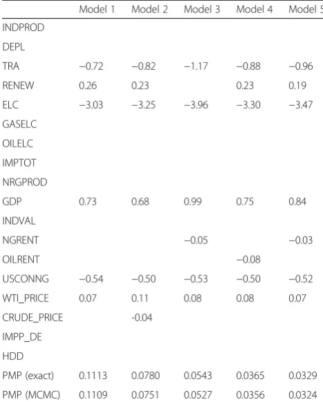
The exact PMP are analytical values, MCMC are simulated values. The PMP is proportional to the mar-ginal likelihood of the respective model, i.e. the prob-ability of the data given the model, times the prior model probability. The best model has a PMP of ca. 11 %. In Fig. 3, the marginal distribution density of the used variables coefficients is depicted. The numerical coefficient estimators correspond with the coefficient values in Table 3. The integral of the densities sums up to the analytical PIP of the regressors, as reported in Table 1.

In order to understand how the distributions are gen-erated, Fig. 4 illustrates the expected values of the best 2000 models generated by the MCMC sampler. These expected values produce the density of the coefficient of

Fig. 1Model inclusion of explanatory variables based on best 2000 models:Red colourindicates a negative coefficient,blue colourindicates a

(10)

the variable CRUDE_PRICE. In other words, every verti-cal grey line corresponds to the expected value of a model (x-axis); the density describes how many models indicate this value (y-axis). The conditional expected value of the variable which is depicted in red (cond. EV) is the analytical value and Cond. EV MCMC is the

sampled expected value. Due to reasonable convergence statistics as depicted in Table 2, the values are rather close to one another.

Although the interpretation of the results is not the main focus of this case study, some explanatory re-marks are provided as an example for other

Fig. 2Posterior Model Size Distribution and Posterior Model Probabilities: model size reflects the number of variables suggested by prior and

posterior distribution of potential variables (mean 7.003). Posterior model probabilities of the best performing 2000 models:blueindicates the sampled model probabilities; inred, the exact probabilities (analytical) are shown (Corr 0.9986)

Table 2Summary of BMA

Mean no. regressors Draws Burn-ins Time No. models visited

“7.0030” “1e + 05” “50,000” “36.3791 s” “29,835”

Modelspace 2^K % visited % top models Corr PMP No. obs.

“262144” “11” “100” “0.9986” “26”

Model Prior g-Prior Shrinkage-Stats

(11)

uncertainty assessments with BMA and Probabilistic Uncertainty. Applied to a specific model, these would indeed refer to the reasoning of assumptions, as dis-cussed in the background section. The posterior inclu-sion probability (PIP) of individual influences depends on the explanatory power of the variable over the whole model space. “WTI Price” with almost 99 % posterior inclusion probability can be interpreted as a reflection of the linkage to oil price developments in natural gas prices. The highest PIP is found in the variable “USCONNG” which is the US Natural Gas consumption,13 what is due to the fact that the re-sponse variable, the natural gas price, is the import price for Germany. If the analysed natural gas price were the end consumer price for households or indus-try, other dependencies could become transparent. Hence, an appropriate choice of the statistical repre-sentation of influences, including considerations of data time resolution and geographical scope of the data is necessary to allow for BMA finding relevant in-fluences for a given energy model. Intuitively, the re-gression model should meet the needs of the subsequently used energy economic model in terms of spatial and time resolution, inclusion of regional vari-ables and the use of a high number of observations is

recommended. For example, if an energy model has a time resolution of 12 time slices a year (summer/win-ter/spring/fall/day/night/peak), the appropriate time resolution could be monthly data, or even daily data if available.

The posterior model probability (PMP) of ca. 11 % seems to reflect a low capacity of the model to repre-sent the observed data. BMA approaches in other contexts should relativize that finding. The example presented by Fernandez et al. for an econometric con-text reports a PMP of 0.3 [45]. The much cited paper of Hoeting, stressing advantages of BMA with respect to classical statistical methods, uses a medical context and reports a PMP of 0.17 in a dataset on primary biliary cirrhosis14 [39]. A PMP of 0.11 for the case study seems thus, even though being low, not un-acceptable. What this means in terms of uncertainty is discussed in the next section.

The BMA calculation method of PMP for a statis-tical model is not new. I chose the method for several reasons. First, it is an approach with solid mathemat-ical formulation as cited. Second, it resolves one of the main problems when dealing with an interrelated target system, as energy models do: what influences the exogenous variable (the input variable) of an en-ergy model. Using the BMA method, the modeller is provided a statistical tool to assess the significance of an influence based on data, and can argue with statis-tical relevance in contrast to pure intuition. This is not to say that intuition can or should not be applied in energy modelling, rather, it can be supplemented by data.

From probability to uncertainty

Communicating an explicit uncertainty assessment, rather than general disclaimers as is current practice, seems necessary because most energy scenarios are presented in great detail in terms of numbers and figures and may thereby suggest a certainty which is possibly not justified. The presented definition of uncertainty departing from probability provides a tool which corresponds to a given energy models re-sults’ in terms of its input variables, its geographical coverage and time resolution. Yet, the method is ap-plicable to very different kinds of energy models (by adjustment of input variables, and potential influ-ences) and is thus also flexible. In the next sections, the application is exemplified with the theoretical concept of the previous sections and the BMA calculation.

The posterior model probability (PMP) can be used to derive the structural, model dependent uncertainty. PMPs are generated with respect to all variables

Table 3Inclusion of variables (coefficient estimate) and posterior model probability for the best five models (rounded)

Model 1 Model 2 Model 3 Model 4 Model 5 INDPROD

DEPL

TRA −0.72 −0.82 −1.17 −0.88 −0.96

RENEW 0.26 0.23 0.23 0.19

ELC −3.03 −3.25 −3.96 −3.30 −3.47

GASELC OILELC IMPTOT NRGPROD

GDP 0.73 0.68 0.99 0.75 0.84

INDVAL

NGRENT −0.05 −0.03

OILRENT −0.08

USCONNG −0.54 −0.50 −0.53 −0.50 −0.52

WTI_PRICE 0.07 0.11 0.08 0.08 0.07

CRUDE_PRICE -0.04

IMPP_DE HDD

(12)

(influences) of a given model. Applying Eqs. 12, 14 and 15, we derive uncertainty as follows.

Ψð Þ ¼A 1−P Að Þ ¼

ΨMγ ¼ 1−p M γjy; X ¼

ΨMγ ¼ 1−PMPMγ

with Model (M) andγ= {1,2,3,4,5} the five best perform-ing models

BMA yields that the model with the highest PMP (thus the lowest uncertainty) includes six variables,

Fig. 3Marginal density distributions of coefficient estimates of the six most relevant explanatory variables: theblue linerepresents the marginal

density; conditional expected values (Cond.EV) are displayed inred solid line, the median ingreen solid line. Thered dotted linesrepresent the double conditional standard deviation (2× Cond. SD)

Fig. 4Marginal density and expected values of models (EV Models) for

(13)

hence, k = 6. In Tables 4 and 5, the results as percent-ages are presented. The uncertainty is calculated straight forwardly from the PMP, the probability speci-fying the explanatory power of the model (the extent to which the influences can explain the dependent vari-able statistically). The model uncertainty of model 1 of approx. 89 % is the uncertainty of the model represent-ing the natural gas price. If model 1 was chosen to rep-resent the natural gas price, the variables would have individual uncertainties of approx. 11 % on average. The individual uncertainties allow an assessment of the explanatory variables and may help to choose the model of lowest uncertainty, or, to consciously include influences with limited explanatory power due to other

considerations.15 To illustrate this, Table 5 depicts model 2, the second-best model in terms of PMP that includes seven of the initial 17 variables. This model choice yields an uncertainty of influences of approxi-mately 19 % on average and a corresponding model un-certainty of ca. 92 %.

Posterior inclusion probabilities (PIPs) are used to de-rive uncertainty of individual explanatory variables, that is, influences. By means of BMA, it becomes clear which variables contribute explanatory power to a model in terms of increased PMP. Applying formula (12) yields the uncertainty of individual influences, hereby taking the inclusion probability the variable k (influence) PIPk has. That is,

Ψð Þ ¼A 1−P Að Þ ¼1–PIPk

Assuming that every variable is supposed to ex-plain the dependent variable with low uncertainty, it follows that variables which perform poorly in terms of explanatory power (i.e. low PIP) should be ex-cluded. However, it may be the case that an influ-ence should be included in an analysis in spite of its low PIP. By individual uncertainties it becomes transparent at what “cost” such an inclusion comes.

The results show that an inclusion of variables which are of little explanatory value to the model in-crease uncertainty. This uncertainty is captured in the lower PMP. In Table 4, the uncertainty assess-ment for model 1 (cf. Table 3) is depicted. The individual uncertainties, (i.e. the uncertainty of influ-ences) yield uncertainties between less than 1 % and almost 50 %. This percentage quantifies to what ex-tent the variable is uncertain in its individual contri-bution to explaining the dependent variable, the natural gas price in the sample space Ω. This is not to say that these variables in general have the calcu-lated individual uncertainty. The posterior inclusion probability yielding the individual uncertainty quanti-fies in how many cases of the Monte Carlo simula-tion of the sample space Ω this variable contributed to an increased posterior model probability (PMP). Within that model, the individual uncertainties further specify the uncertainty whether a specific in-fluence contributes to explaining the data of the dependent variable.

Please note that one can use any statistical data suspected to influence the input variable of an en-ergy model. I argue that the assumption is not well justified if the probability of these influences explain-ing the input variable is low and, consequently, its uncertainty is high. For example, if a natural gas price assumption in a fictive energy model (with a scope adequate to the data used for this BMA

Table 4Individual uncertainties of variables (influences) and model uncertainty for model 1 (cf.Table 3) withn= 6

Model 1M1

Variablek PIP Individual uncertainty n

USCONNG 99.24 % 0.76 % 1

WTI_PRICE 98.62 % 1.38 % 2

ELC 97.07 % 2.94 % 3

TRA 95.46 % 4.55 % 4

GDP 95.20 % 4.80 % 5

RENEW 50.83 % 49.17 % 6

Averaged uncertainty

Xk¼n k¼1ð1−PIPkÞ

n 10.60 %

PMPM1 Model uncertainty

11.13 %

Model uncertaintyΨ(M1) = 1−PMPM1 100 %−11.13 % = 88.87 %

Table 5Individual Uncertainties of variables (influences) and model uncertainty for model 2 (cf.Table 3) with n = 7

Model 2 M2

Variablek PIP Individual uncertainty n

USCONNG 99.24 % 0.76 % 1

WTI_PRICE 98.62 % 1.38 % 2

ELC 97.07 % 2.94 % 3

TRA 95.46 % 4.55 % 4

GDP 95.20 % 4.80 % 5

RENEW 50.83 % 49.17 % 6

CRUDE_PRICE 30.69 % 69.31 % 7

Averaged uncertainty

Xk¼n k¼1ð1−PIPkÞ

n 18.99 %

PMPM2 Model uncertainty

7.8 %

(14)

calculation) were justified referring to developments in US natural gas consumption (USCONNG), oil prices (WTI_PRICE), electricity consumption (ELC), road sector energy consumption (TRA), GDP, and combustible renewables and waste (RENEW)—model 1—than the statistical uncertainty that these develop-ments impact the assumption would be 89 %. This renders transparent whether assumptions are well justified on statistical grounds and provides an expli-cit assessment for recipients of energy model results.

From model to prediction

BMA densities can not only be applied for inference but also for a prediction based on historical data. The Bayesian regression can be used to calculate predictive densities, similarly to the coefficient densities. Predict-ive quality can be used to investigate how well the model performs, given real data are available. For the present exercise, the same BMA parameters as de-scribed above are used, with 1e + 05 draws of the MCMC and a burn-in of 5e + 04. The 26 observations of the dataset are split in order to predict the last two observations, i.e. the natural gas price in 2008 and 2009.16 For a detailed analysis of the predictive per-formance see Chua et al. [46], for a prediction exercise with dynamic factor models [47].

In Fig. 5, the predictive density and the real value of the natural gas price for observation 25 (2008) are depicted. Response variable on the abscissa is the natural gas price which was called dependent vari-able and is the input varivari-able to an energy model. The predictive density on the ordinate shows where—with respect to the BMA model chosen— -natural gas price assumption should be settled given

the influences. The predictions underestimate the natural gas price cf. Table 6. A detailed analysis could explain whether the two real values are out-liers. The associated uncertainty for the model (cf. Table 4) already indicates that prediction results can be expected to be rather poor.

This is a notably coherent approach when key as-sumptions are to be chosen for input variables in quantitative terms. When defining storylines for sce-narios, the need for quantitative assumptions arises. Using predictive densities for input variables can be employed to find the numerical values for assumptions based on statistical data. Not only become the implicit assumptions about the variable context in the target system explicit (and can be communicated to recipi-ents), but also a value for the assumption that respects past observations can be retrieved. Valuable informa-tion of the predictive density are the form (well-shaped), the standard errors (0.36 for 2008 and 0.319 for 2009) and the expected value that could be used to formulate a statement of the form: “With an uncer-tainty of at least 89 %, the natural gas price lies be-tween 11.44 and 9.97 US dollars per million Btu. This estimation is based on six influences on the Natural gas price over a period of 24 years.”

From uncertainty of input variables to uncertainty of energy model results

The assessed uncertainty of input variables to energy models can subsequently be used to formulate a lower bound of the associated uncertainty of energy model re-sults, under the introduced premise that the output of an energy model cannot be less uncertain than the input.

ΨEnergy Model Output ≥ ΨInput Variable ð16Þ

A statement of the form: “Given the input vari-ables used in this energy model, the results and fore-cast statements from it are uncertain by at least 89 %. Relevant influences on the input variables which can be analysed statistically indicate this un-certainty.17” The statement could be further refined for specific input variables and energy model results which can be appointed to these inputs. In general, the least certain input variable should determine the

Fig. 5Expected value and predictive density: The predicted density

of the natural gas price (response variable) in predicted observation 25 (2009) is shown. The real natural gas price (realizedy) is represented by theblack dotted lineand double standard errors (2× Std. Errs) indicated asred dotted lineof the expected value (exp. value). The expected value based on BMA is shown asred solid line

Table 6Prediction of last two observations of the data set

Observation 25 26

Expected value 10.71 7.27

Real value 11.56 8.52

(15)

uncertainty statements. In particular, if decision sup-port is aspired and explicit recommendations are formulated, recommended measures should include an uncertainty assessment for relevant variables con-cerning the measure.

It seems necessary to clarify that such an uncer-tainty assessment should not be perceived as tool to attack the credence of energy model results. Quite contrarily, quantifying uncertainty should render model results more realistic in the light of a con-stantly changing, interrelated and non-deterministic target system. Any other methodology of decision support for mid- and long-term future choices sup-posedly will have comparable difficulties anticipating developments. Even with (very) high associated un-certainty, energy models can be of (relativised) value in decision support after all.

If model-based statements, projections and recom-mendations are used in policy advice, it is necessary to accompany these statements with an indication of how dependable they are. Transparency in the model-ling process and evaluation by recipients would be improved, if energy model results were communicated with their associated uncertainty (Eq. 15), context de-pendency (influences deemed relevant), and explicit assumptions (numeric assumptions of influences for prediction).

The aim of the case study is to exemplify how a quantitative assessment with the BMA method and Probabilistic Uncertainty for input variables to en-ergy models could work. The presented modelling choices are not meant to be a unique solution; ra-ther, the approach could be developed along these lines. Software solutions other than R could be applied.

Results

In summarising the findings of the case study, the main observation is that by applying Probabilistic Uncertainty and BMA method, a quantitative assess-ment of uncertainty in terms of input, parameter, and context uncertainty is possible. The embedded nature of input variables in other systems and be-yond energy model boundaries is referred to as “ con-text” and can be analysed by suitable choice of potential explanatory variables, called influences. Among the small database used for this case study, significant influences on the natural gas price are consumption in the USA, crude oil price, electricity power consumption, road sector energy consump-tion, gross domestic product and the share of com-bustible renewables and waste in total energy consumption.

The results suggest that the natural gas price as an input variable holds an uncertainty of at least 89 %, given the data used. Clearly, as this case study was not designed for a specific energy model, these find-ings cannot be applied to an energy model. For an application to a specific energy model, the regional scope, time resolution and sectorial (dis-)aggregation of influences must be chosen accordingly. It is im-portant to note that—as with all statistical analy-ses—long observation periods and reliable data sources increase the quality of the assessment, as it reflects reality more accurately. This paper is not fo-cussed on the interpretation of results but rather on a presentation of the practical aspects of the method. The case study has an exemplifying charac-ter and could be used as a reference for an uncer-tainty assessment with suitable data for a specific energy model.

However, based on the case study, some general analyses can be formulated. It seems that at least some input variables to energy models are highly uncertain with respect to influences bearing on them. Those influences which can be estimated by statistical methods seemingly explain (at least some) input variables of energy models with little probability. The conjecture is that resorting to gen-eral disclaimers, as it is common practice, does not reflect the high uncertainty that is associated with individual energy model results. The presented ap-proach could provide an energy model specific, ex-plicit and understandable uncertainty assessment which could accompany energy scenarios and ren-der associated uncertainties tangible for the recipients.

Discussion

According to Walker et al. statistical uncertainty is the least ignorant of all uncertainties involved in models. It thus seems reasonable to use statistical data for uncertainty assessments. However, subjective expert knowledge should be included and the method can accommodate this by prior probabilities.

(16)

used in decision support, as presented, for example, the IEA states this in their self-presentation [20]. It seems reasonable and good scientific practice pro-viding an uncertainty assessment if energy scenarios are to be the basis of policy-making, planning and investment decisions. Recipients may hold an unjus-tified confidence in “projections” or scenarios sug-gest by studies, if uncertainties are not analysed in detail. One key argument of energy models is that if all assumptions hold, the development would be as presented in the energy scenario. The proposed approach can render transparent whether statistical evidence is lacking for this argument. First, it is highly unlikely that all assumptions hold, given there can be hundreds in an energy model. Second, even if all assumptions hold, the method potentially proves that for at least some assumptions (the assessed input variables), the assumed cause-effect-relations are statistically highly uncertain. If not, the better, for energy model results would be affiliated with an uncertainty assessment proving its reliability statistically. To give an example, the specific as-sumption of the input variable “natural gas price” can be justified with developments in production and consumption patterns (the influences), yet given historical data, it may prove that these develop-ments did not explain the value. If it can be justi-fied by the influences, the uncertainty assessment provides statistical evidence.

Another limiting aspect if it comes to large and complex models, it is the parametric nature of the proposed uncertainty assessment. An intelligent choice of input variables which are analysed seems necessary, given that large models employ thousands of assumptions. This could be done in several ways. For one, the most influential input variables could be chosen, possibly determined by a sensitivity ana-lysis. This approach proved successful in the NUSAP method [23]. Or, if tracking of input variables across the energy model processing is possible, the number of variables that are assessed could be limited. Yet another possibility departs from model-based recom-mendations, which should be based on a specific model result, and that result should be evaluated with respect to its uncertainty. In other words, if a model-based energy scenario is publicly presented, it should be accompanied with an uncertainty assess-ment for the variables which are the basis for rec-ommendations. Typically, these would be the exogenous variables presented in the storylines, or definitions of scenarios, as for example, the numer-ical key assumptions in the “New policies scenario” in the World Energy Outlook by the IEA [37]. It is possible that some input variables are less uncertain

than others, in which case, the most uncertain input variable should provide the lower bound (with refer-ence to the premise that output cannot be less un-certain than input to the energy model). It is not claimed that the presented example of an input vari-able (the natural gas price assumption) is the most important assumption of an energy system model. It is chosen for it is a typical assumption which is de-cisive for energy model results, in particular, if an optimisation model is used with an economic ration-ale, as are other price and cost assumptions, be it of fuels or technologies. The uncertainty assessment of input variables is indeed work, statistical work and computational work. However, if one aspires an un-certainty quantification (rather than a general dis-claimer) with a solid method, it cannot be achieved through one assessment for an energy model, neither quantitatively nor qualitatively (the number of expert elicitations in qualitative assessments may render proof ). Also, it would not do justice to highly de-tailed energy models, which might well profit from the possibility to analyse specific input variables in terms of their uncertainty.

(17)

there is none, it is questionable how the energy models which themselves assume functional rela-tions can be justified. The presented approach pro-vides a quantitative explicit tool that is adjustable for different energy model types (their input vari-ables and influences bearing on them), and flexible in the definition of the functional mathematical re-lation of influences on an input variable.

The computational effort for the presented case study was reasonable, taking approx. 10-min calcu-lation time with the used software. All graphs are standard functionalities of the R BMS package. Data collection and preparation is indeed more time consuming. It is suspected that energy model-lers would already dispose of much relevant statis-tical data for calibration purposes from reliable sources.

The method, as any statistical method, assesses probabilities based on past events. This implies that the expectation and focus of future develop-ments is in a sense limited. However, the energy models operate within the same set of assumptions and expectations, which is why this method does not determine the future but rather provides ex-pectations based on the past. A statistical analysis is always focussing on the past. The implicit as-sumption is that relations in the past are at least likely to hold in future. This must not be the case. But given that the energy models are also cali-brated with and based on statistical data, the ana-lysis is consistent with practices in energy modelling, less subjective than expert elicitation and more specific than general disclaimers.

The method can be criticised for an idealisation inherent to all modelling techniques. The assump-tion that the sample space Ω can be known in its entirety does not hold from a realistic point of view. It is not possible to know and account for all thinkable and hence possible alternative events (which by definition comprise uncertainty). Given that an energy model is confronted with the same arbitrarily defined sample space, it is equally mean-ingless to compute a projection or forecast with an energy model as it is to assess its uncertainty. However, if the energy models are used, it becomes meaningful to assess their uncertainty within the model’s sample space. The approach has the dis-tinct advantage of analysing the relevance of poten-tial influences in statistical terms and subjective expert knowledge (by means of prior specification), in contrast to a purely subjective uncertainty as-sessment as expert elicitation. However, experts may have a clear intuition which influences affect an input variable of an energy model.

Analysing these influences in terms of BMA and Probabilistic Uncertainty may render some intuitive over- or underestimations transparent.

The energy models may have time horizons of decennia, and the question arises, whether the un-certainty assessed by the proposed approach is stable for energy model results in the long-term future. Indeed, it is not. Uncertainty is expected to be higher, the further in the future, a model-based statement is settled. If, for example, an energy study promotes a specific energy system state in the year 2040, the uncertainty is expected to be higher than the uncertainty 1 year from now. Un-certainty over time of assumptions means that if a model has a modelling horizon, and model results are displayed as time series, the related uncertainty of the results must increase towards the end of the horizon in future. As stated above, this is due to the facts that model inherent simplifications and generalisations perform error propagation and that assumptions regarding mid- or long-term future cannot be verified or falsified with available tests at present time. Note, that the related uncertainty increases the further in the future an assumption is made. Let A be an assumption with a time index x, x= 1,2,3,…,n. The time index is to be read as some sort of regular time interval, e.g. hour, month, or year. Further, assume that a model is comprised of different assumptions A, each of which is time dependent. An assumption A, as the

natural gas price, in 1 month from now is

(18)

that an uncertainty analysis based on statistical data may give an evaluation of the lowest uncer-tainty indicated by statistics, and that some energy model results may be more uncertain.

Conclusions

The presented Bayesian approach for uncertainty quantification in terms of assumption probabilities al-lows an uncertainty assessment of input to energy models.

In the first section, the question where uncer-tainty is present in energy models and why it should be addressed was discussed. This discussion should raise the awareness that energy model re-sults are highly dependent on input assumptions. The practice of “general disclaimers” seems unsatis-factory, especially, if model-based statements are used for policy advice and decision support creat-ing far-reachcreat-ing social, economic, and environmen-tal consequences.

The next section provided a definition of uncer-tainty. The probabilistic uncertainty measure de-fined allows quantifying uncertainty in a coherent manner with probability theory. The distinct advan-tage with respect to commonly used qualitative as-sessments is an unambiguous representation of uncertainty, which is understandable without tedi-ous lecture of explanatory notes. “The probability that a statement might not be true is at least Ψ (e.g. 89 %)” seems more explicit and understand-able than commonly used “likely”, “very likely” and the like cf. [48]. Intentionally, the approach relies on established methodologies (BMA) and concep-tual frameworks (probability theory) to derive such quantitative statements. Another advantage is a consistent and transparent quantitative interpret-ation of implicit assumptions as predictive densities for assumptions of input variables to energy models.

Finally, the presented case study aimed at exem-plifying how the approach in practice could work. Indeed, specifications of BMA such as the chosen sample-routine or the prior choice should be dis-cussed individually for a specific input variable of an energy model. The case study illustrates how the approach could add to the tools of uncertainty quantification in energy modelling.

Further research should include practical specifi-cations of the approach and legitimate inference from uncertain energy model results. A comparison of the different energy models could be carried out to evaluate their associated uncertainty.

Endnotes

1

Typical model horizons are short term: hours up to days, mid-term: up to 2030, long term: up to 2050 or 2100

2

Assuming the” Law of Demand”, i.e. the quantity demanded depends negatively on price, ceteris pari-bus. This is a very useful and convenient theory, as long as the ceteris paribus assumption is not ignored, and it is understood that complements as well as sub-stitutes exist for most traded goods, as Bierens and Swanson note [55].

3

In contrast to aleatoric uncertainty, for example, nat-ural variability, which can be modelled by stochastic techniques cf. [56].

4

This step could involve a sensitivity analysis in order to reduce the amount of input variables when large models are evaluated. See also limitations and discussion of the approach.

5

Note that by condition 1 and 2ℱ is closed under fi-nite intersections.

6

Other measures, such as a Popper-measure would be thinkable, allowing for conditionalization on zero-probability events. The benefit of such a definition is left to future work.

7

The proof is omitted but can be found in most lecture notes on probability and measure theory, e.g. [57, 58].

8

In the case study, this influence is represented by the explanatory variable NG_rent, the difference between the value of natural gas production at world prices and total costs of production.

9

Data and inferences from them are not the focus of this text, rather a discussion of the methodology and its application in the field of energy economics is sought. A coherent database with as many observa-tions as possible should be applied in an uncertainty assessment for a specific input variable of an energy model.

10

In the following, the terms regressors, explanatory variables, and influences are used interchangeably.

11

This translates to “BRIC” g-prior in the modelling exercise

12

For other options such as reversible-jump sampler for BMS model package in R, see [38].

13

See Appendix. 14

Which is used for medical treatment, nota bene. 15

For example, based on expert knowledge one could choose to include an influence that is expected to be-come more relevant in future than it was in the past.

16

For source information refer to the appendix. 17

Of course, the influences should be detailed too. 18

(19)

Appendix

Used data is freely available from the following sources. However, consistent data with more observations of in-fluences deemed relevant is recommended if the focus lies on interpreting results.

Table 7Explanation of abbreviations of influences for the case study and source of data

Abbreviation Influence Unit Source

GN_Price Average German import price [US dollars per million BTU] [21]

INDPROD Production of total industry in Germany“DEUPRODINDAISMEI” seasonally adjusted

Index 2010 = 100 [49]

DEPL Adjusted savings: energy depletiona _{[current billion US$]} _[₅₀_]

TRA Road sector energy consumption [% of total energy consumption] [50]

RENEW Combustible renewables and waste [% of total energy] [50]

ELC Electric power consumption [1000 kWh per capita] [50]

GASELC Electricity production from natural gas sources [% of total] [50]

OILELC Electricity production from oil sources [% of total] [50]

IMPTOT Energy imports, net [% of energy use] [50]