R E S E A R C H
Open Access
Novel neural network application for
bacterial colony classification
Lei Huang
1and Tong Wu
2**Correspondence: wutongpkuhsc@pku.edu.cn 2Peking University Health Science Center, 38 Xueyuan Road, Beijing, China
Full list of author information is available at the end of the article
Abstract
Background: Bacterial colony morphology is the first step of classifying the bacterial species before sending them to subsequent identification process with devices, such as VITEK 2 automated system and mass spectrometry microbial identification system. It is essential as a pre-screening process because it can greatly reduce the scope of possible bacterial species and will make the subsequent identification more specific and increase work efficiency in clinical bacteriology. But this work needs adequate clinical laboratory expertise of bacterial colony morphology, which is especially difficult for beginners to handle properly. This study presents automatic programs for bacterial colony classification task, by applying the deep convolutional neural networks (CNN), which has a widespread use of digital imaging data analysis in hospitals. The most common 18 bacterial colony classes from Peking University First Hospital were used to train this framework, and other images out of these training dataset were utilized to test the performance of this classifier.
Results: The feasibility of this framework was verified by the comparison between
predicted result and standard bacterial category. The classification accuracy of all 18 bacteria can reach 73%, and the accuracy and specificity of each kind of bacteria can reach as high as 90%.
Conclusions: The supervised neural networks we use can have more promising
classification characteristics for bacterial colony pre-screening process, and the unsupervised network should have more advantages in revealing novel characteristics from pictures, which can provide some practical indications to our clinical staffs.
Keywords: Bacterial colony, Classification, Convolutional neural network, Clinical laboratory
Background
The rapid development of computational imaging processing systems has largely ben-efited the hospitals for image analysis in diagnosis and investigation. Most of these technologies are applied to facilities such as usage in iconography: ultrasonography, CT, SPECT and MRI [1–4], but few of them has been used directly as a computational vision method in bacterial classification. While there are some limitations of the traditional bac-terial classification methods which depend on clinical expertise in very diverse colony structures of different bacterial species [5]. Firstly, they are time-consuming and laborious
© The Author(s). 2018Open AccessThis article is distributed under the terms of the Creative Commons Attribution 4.0 International License (http://creativecommons.org/licenses/by/4.0/), which permits unrestricted use, distribution, and reproduction in any medium, provided you give appropriate credit to the original author(s) and the source, provide a link to the Creative Commons license, and indicate if changes were made. The Creative Commons Public Domain Dedication waiver (http://
for staffs [6]. Secondly, the identification needs enough morphology expertise of bacte-rial colonies, which is difficult for beginners to tackle with. Therefore, the development of an automatic bacterial colony morphology identification system is helpful for aiding clinical staffs in reducing workload as well as acting as a reference for beginners. Some literatures have presented the useful features to identify different bacterial species such as shape, size, surface, border, opacity and color [7], with the combination of staining methods, such as Gram Staining [8]. While the discrimination of bacterial strains from a large amount of samples is still very complicated. The traditional manual discrimina-tions based on expert classifying experience of circular or irregular colony shape, convex or concave colony elevation, etc., require lots of manpower and clinical expertise, espe-cially in the situation with large amount of samples in a tertiary hospital. And a framework based on bacterial colony morphology data can be a convenient way for supplementing the preliminary identification process. It is really necessary to build up this computational vision framework, which can automatically classify lots of bacteria as the preliminary screen preparation results. These results are able to be utilized to narrow down the clas-sification scope in the following more advanced and specific identification procedure such as utilization of VITEK 2 system [9] and MALDI-TOF mass spectrometry detection system [10].
Deep learning system is a kind of machine learning method based on learning data rep-resentations [11], and one of its applications is computational vision. For computational vision, it mimics the arrangement of neural network in human brain, which can learn and transport different qualities of information through multiple layers of transforma-tion [12]. It can get feature representations by automatically learning from raw images without applying human experience, and it can model these abstract features by using constituent multiple non-linear transformations. The convolutional neural network is one of these machine learning methods that mimics the connectivity pattern between neurons of visual cortex [13]. It can extract hierarchical image feature representations based on multi-layer processing. And the features extracted are able to have a better performance than that from hand-crafted features because they are more general and less subjective.
In this study, feature representations of colonies from 18 bacterial species were learnt to build convolutional neural network. Commonly, preliminary bacterial classification was given out as training labels by human experience of bacterial colonies in clinical laboratory. Then these labels could be aligned with specific features of bacterial species extracted from our networks, which could be recorded and be further applied for our networks prediction. The building of one computational classification model depended on supervised images with standard labels, while the building of the other model relied on unsupervised images which were only for this neural network to extract colonial fea-tures. The predicted labels and annotations from both neural networks are quite useful because they can provide some aids for the operation of clinical laboratory and they are able to show inspirations of bacterial colony classification to clinical staffs based on their extracted features.
Methods
designed by the SuperVision group for large scare visual recognition [14]. Besides the input layer and output layer, both these two CNN models are generally consisted of four types of layers, which is convolutional layer, ReLU layer, pooling layer and fully connected layer. The function of each layer and detailed processes of training are given in the follow-ing part. Then, a kind of unsupervised method named Autoencoder is introduced, and its general structure and detailed training processes are presented, to make comparison with the supervised methods and to verify the feasibilities of both methods.
Traditional convolutional neural network
General structure: Our convolutional neural network has basic architecture built with multiple distinct layers, having their own unique functions to transform input volumes to output volumes. Besides the input and output layer, there are some hidden layers in between that play the most important part in filtering and transporting information. These are convolutional layer, pooling layer and fully connected layer. Convolutional layer has a set of learning filters, and each filter has many receptive fields that expand through the whole filter of the input. Depth of a convolutional layer is the number of neurons in a layer, and each neuron is able to extract a specific feature detected from positions of the input. A 2-dimensional feature map is constructed based on these features, and it will have spatially local correlation with neurons of next adjacent layer by receptive fields, a spatially connectivity pattern. Thus the feature map will act as the input of the next layer, and each output volume can be represented as a neuron output that projects to a small region in the input. In this way, spatial image information is extracted and transported by multiple connective layers. While because of so many parameters and large size of the convolutional network representation, pooling layer is proposed to reduce both values to decrease computational load as well as avoid over-fitting. During the processing of pool-ing, the number of neurons in each layer, the depth of dimension remains unchanged, only the size of each depth slide will be reduced. Finally, at the end of some convolutional layers and interspersed several pooling layers, all activations are gathered in one layer, the fully connected layer. Considering the input signal, weight and bias together, this fully connected layer can generate the output value. Depending on this, fully connected layer can do the high-level judgement for bacterial classification.
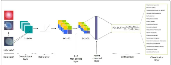
Each layer: In our convolutional network classification model, there are totally seven layers which represent different functions successively, and the general scheme of these connected seven layers network is depicted in Fig.1. There are image input layer, convo-lutional layer, rectified linear layer, max pooling layer, fully connected layer, softmax layer and classification layer, respectively.
Fig. 1The general structure of the conventional neural network
is 3-by-3. We choose this small scope of size because the discriminations among different kinds of bacteria is subtle, such as different shape of margin of colonies, for the reason that small scopes of filters can have a better characteristics to highlight the fine variations among bacterial colonies. To fully represent all features of the bacterial colony image, we set the number of filter as 50, which means that there are equivalently 50 neurons that can extract, evaluate and transport 50 kinds of information into the next layer of visualiza-tion. When the input volume of images has been transported through the convolutional layer, the dot products are calculated between the entries of filters and the input. From the dot product map, the convolutional layer can detect some specific features at some spatial spaces in the input layer, and these detected features will serve as an activation of filters. We combine all the activated filters together to activation maps, which are able to act as the output volume of this convolutional layer.
The following layer of the convolutional layer is the ReLU layer, which is for rectifying the convolutional output volume by linear function. The processing function in this layer can be written asf(x) =x+ = max(0,x), which can help remove negative values in the convolutional output and do linear amplification to positive values [15].
We set a pooling layer after processing of the rectified linear unit. It is responsible for reducing the spatial dimension from the output of previous convolutional layer, and it aims at decreasing computational overhead and load as well as avoiding over-fitting for lots of parameters to consider. Here the pooling method we utilize is the max pooling algorithm, which can screen the input image with rectangular region and then figure out the maximum element in this region. The height and width of this screening rectangular region is 2, and we also set the stride, number of elements for moving along the image horizontally and vertically, as 2. In this way, as the dimension of stride being equal to that of the screening region, in every period of screening there will be no overlap between these screening regions.
we denote the set of observed data byxand the set of parameters byθ. The recognized probability of each classification would be:
P(cr|x,θ)=
P(x,θ|cr)P(cr)
k
j=1P(x,θ|cj)P(cj)
(1)
HereP(cr)is the prior probability of class r, and thekj=1P(cj|x,θ)is equal to 1 [16]. Then the returned probabilities by this activation function will be assigned to each exclusive class by final classification layer.
Detailed training: The set of parameters for training and the selection of training algo-rithm are essential for the feasibility of this model building and application. Here we set the algorithm of training as stochastic gradient descent with momentum, the number of circles on the whole training data as 30, and the initial learning rate as 0.0001. When we get the error function that is calculated from the entire training data and the output train-ing prediction after several traintrain-ing iterations, the stochastic gradient descent algorithm is able to minimize the error functions by taking steps in the fastest gradient descent directions [17]. We assume one parameter of the training model isa, the calculated error function isE(a), and the learning rate isμ, thus the i+1 times of modification of this parameter can be expressed as:
ai+1=ai−μ∇E(ai) (2)
And a momentum term, which is how much the parameter from previous step contributes to current iteration, can be added to this equation so as to prevent the error function E(a) from oscillating around several steepest descents to the objective function [18]. Assume the σ as the coefficient of contribution from parameter in previous iterations to the current iterations, so the modified function can be written as:
ai+1=ai−μ∇E(ai)+σ(ai−ai−1) (3)
This momentum term can be explained from an analogy to momentum in physics, that would cause acceleration from the gradient of the force, so as to travel in the direction which is able to reduce oscillation [19].
Another issue is that we have 18 classifications and 18 dataset of observations, and the whole error functionE(a)can be divided into the sum of error functions from each dataset,1kkj=1E(aj). In this way the parameters can be updated by minimizing the whole error function through stochastic gradient decent algorithm, and calculating the gradients of the parameter of current iteration with backpropagation algorithm. By getting these gradients as input and updating them to minimize the error functions again and again, the neural network training model can be built to mimic the entire training data in an optimal way.
AlexNet neural network
network, to solve this classification problem. As AlexNet neural network is a kind of con-volutional neural network, the general structure of this network also consists of image input layer, convolutional layer, pooling layer, fully connected layer, and etc. However, the AlexNet neural network is much deeper compared with common convolutional neural network, which has more channels of convolutional layers and gathering layers of these multi-channel layers to collect and normalize information [20]. And these specific lay-ers of AlexNet neural network can be called cross channel normalization layer. What is more, as the distributions of convolutional layers are different, there are many convolu-tional layers from different channels set at the second layer of the AlexNet so as to extract more features from images, and after a set of pooling layers there will be a series of dense convolutional layers, that is these featured convolutional layers will stack on top of each other without any pooling layer inserting in the middle [21].
Each layer and detailed training: We have a total of 25 layers in this AlexNet archi-tecture. The first layer is the image input layer for dimensions of 227×227×3 images. The next are two convolutional-ReLU-cross channel normalization-pooling layers’ cir-cles, with following condensed convolutional layers and ReLU layers. The dimensions of convolutional layers in the first two circles are 11×11×3, 5×5×48, and 3×3×256, respectively. And dimensions of subsequent dense convolutional layers are 3×3×192, 3×3×192 in order. The following are fully connected layers with insertions of ReLU lay-ers and dropout laylay-ers. In the end, they are softmax layer and classification layer, which are similar with that in our previous convolutional neural network. The dropout layer in this AlexNet architecture is to dropout half of the trained neurons randomly, which is responsible for reducing the computational load, especially for this multi-channel con-volutional neural network, but it will not decrease any parameters calculated from the training process. The multi-channel design coupled with dropout method will effectively prevent over-fitting and long computation time. That is also an essential improvement of the AlexNet to deal with large amount of training data.
The application of this AlexNet network is not to train the network from the very begin-ning, but to adapt it to our application. Thus after getting the training data from half of the entire data, we choose the 20th layer, the second fully connected layers array, of the net-work to extract features from our training image data. Because the layer array we choose is the 4096-element fully connected layer, we can get a 4096-element feature from each image, and we set this 4096×2491 feature matrix as thetrainingfeaturesmatrix. Next, for this supervised learning model to be built, we label every image from the 2491 with their standard bacterial categories. By combing thetrainingfeaturesmatrix and the labeled cat-egorical matrix together, we can build a support vector machine (SVM) classifier. This algorithm can efficiently perform a non-probabilistic binary linear classification as well as a non-linear classification with kernel trick. Based on qualities of AlexNet network and SVM algorithm, a complicated and efficient classifier which is suitable to deal with large amount of data and more classifications is built.
Unsupervised Autoencoder neural network
anomalies, we use both supervised and unsupervised machine learning methods to tackle with this classification problem. For the unsupervised artificial neural network, we apply the Autoencoder neural network, which can extract features automatically with unlabeled bacterial colony images.
Our Autoencoder has one input layer, one output layer, and some hidden layers con-nected between them. The number of nodes in the input layer is the same as that in the output layer, with a feedforward, non-recurrent training direction. Another feature of this Autoencoder neural network different from convolutional neural network are the encoder and decoder parts [22]. In this case, every input valuexfrom input space will be weighted with a weight matrixWto get the code:
z=α(Wx+δ) (4)
Herezis the corresponding code, the latent variable isx,αis the activation function for this input, andδis the bias vector. After encoding, the decoder layer would transfer the zmap to the structure of output space ofx´, which has the same dimension as the input space ofx.
´
x= ´αW z´ + ´δ (5)
And by backpropagation algorithm, eachx´value from output space will be made similar to thexvalue from input space by adjusting the identity function. Thus the error function ofxandx´can be built as [23]:
E(x,x´)=x− ´α(W´(α(Wx+δ))+ ´δ)2 (6)
By minimizing the error function and updating the weights, this model can improve its performance continuously.
Each layer and detailed training: There are several components for the model con-stitution. The hidden units in the first hidden layer are 800, which is forced to learn a compressed features from the input. The dimension of our input image 50×50×3 is much larger than 800, which makes the encoder layer be able to learn more significant features for the bacterial colonies discrimination. The training epochs we set in the first hidden layer, in the encoder layer is 400, the weight of each element in the input space as we describe above is 0.004, and the average output of each neuron in the hidden layer is 0.15. After encoding, the decoder layer will try to reverse the mapping to reconstruct the original input.
After getting the extracted data from the hidden layer of the first Autoencoder model, we can build a second Autoencoder model with the similar way. The difference of this second Autoencoder is that it does not utilize the training data but taking use of the fea-tures from the first Autoencoder model instead. The input size of the second Autoencoder model is even smaller, and it can give out smaller representative features of the colonies. Here the dimension we reduce by the second Autoencoder is 200, and the final layer is the 18-dimensional layer aiming to classify these 200-dimensional vectors into 18 digit classes.
images into this stack neural network and visualize the accuracy with a confusion matrix. We can also use backpropagation manually to improve the tuning of this multilayer net-work, and it can be seen from the statistical results that the performance becomes much better.
Results and discussion
In this paper, three popular neural network algorithms have been used for training and testing the bacterial colony classification models. The feasibility of these proposed models has been evaluated in terms of the standard classification of bacterial images from clinical database.
Dataset
The utilized dataset for these proposed models has been collected from clinical micro-biology lab of Peking University First Hospital and classes are given based on the species of these bacterial, such asEscherichia coli,Klebsiella pneumonia,Staphylococcus aureus, Pseudomonas aeruginosaand etc. There are totally 18 classes of bacterial colonies in this dataset, which all belong to the most common human pathogenic bacteria. The total number of every bacterial class in this dataset is 4982. And the images from each class have been divided into both training and testing sets. The percentages of images for training set and testing set are both 50%. 2491 images are used in training set and 2491 are used in testing set, respectively. The input images for the convolutional neu-ral network and the AlexNet neuneu-ral network have the 100×100 dimensions with colors, and the input images for the unsupervised Autoencoder neural network have the dimen-sion of 50×50×3, which would greatly reduce the computational load for this model. And some examples are given in this paper shown as Figs.2 and 3 which represents the differences among different classifications and variations among individual images of each class.
Fig. 3Images fromStreptococcus agalactiaeclass showing the intra variations
Classification performance
To evaluate the performance of these three models, we use several parameters, the true positiveT+, the false positiveF+, the true negativeT−and the false negativeF−. The sensitivity, is the model to correctly classify the bacterial colonies into their species, can be expressed as [24]:
Sensitivity= 1 18
18
j=1
T+
T++F− (7)
The specificity for correctly rejecting bacteria to classifications that are not belonging to, has the expression as:
Specificity= 1 18
18
j=1 T−
T−+F+ (8)
And the precision and accuracy of each model have the expression: Precision =
1 18
18
j=1 T
+
T++F+ andAccuracy=
1 18
18
j=1 T
++T−
for description and discrimination, so that the precision and sensitivity can be affected. The misclassification may be generated from our sample variations, which may be intro-duced from bacteria living in different maconkey agar or blood agar. And it also means the repeatability of our models prediction is limited, maybe due to small number of neu-rons being integrated for classification. When the number of neuneu-rons for judgement is not enough, it will make the features representing for one bacterial species localized, which makes it hard to integrate enough feature weights to give a comprehensive judgement. In addition, these three models have many false negative values and few false positive ones which lead to overall low sensitivity and high specificity [25]. The range of sensitivity is from 0.069 to 1.000, and the species with lowest sensitivity value isEnterococcus faecalis, as excepted. However, the specificity of each bacteria is very high which can commonly reaches more than 0.950. This phenomenon may be because the number of neurons for giving bacterial category in fully connected layer is not enough, the screening process will be less strict to identify many false negative values. In this way, the not excluded false negative values will make the denominator bigger and the sensitivity lower. In another way, this less strict classification models can lead to lower false positive values and higher specificity. Thus they can serve their benefits of alerting clinical staffs to the situation when they classify some colonies into dangerous species.
Comparison
To evaluate the feasibility of each deep learning based framework, the performance com-parison was made among these three neural networks- conventional CNN, AlexNet and Autoencoder. According to accuracy and precision results, CNN and AlexNet methods are comparable, both having better precision performance than Autoencoder. This maybe because unsupervised neural network will extract some features that are not specific for bacterial classification, such as the features of agar background. For sensitivity and speci-ficity, the two supervised networks also work better, and AlexNet has higher sensitivity than conventional CNN which maybe due to its highly compressed convolutional layers. Thus we can conclude that the supervised neural networks have more promising clas-sification characteristics for bacterial colony application, and the unsupervised network should have more advantages in revealing novel characteristics from bacterial colony morphology [26].
Clinical bacterial colony features
Fig. 4Bacterial colonies’ features extraction from the conventional convolutional neural network
the Autoencoder neural network will give us more intuitive discriminations about bacte-rial colonies, which seems that the shapes and the edge-like information of the bactebacte-rial colony are on the foreground of the extracted features that this neural network system is going to take into consideration. And we can learn some classification strategy from this for clinical bacterial colonies recognition.
Performance evaluation of statistical results
Statistical results of classification of our unsupervised CNN are shown in Table1. Because the unsupervised neural network is based on the natural morphologies of colonies’ fea-tures, we can learn some information about classification from them. There are different classification performances among different bacteria. TheStaphylococcus aureushas the
highest classification accuracy in the output class, while theKlebsiella oxytocahas the highest probability to misclassify. This may becauseKlebsiella oxytocacan grow in both maconkey and blood agar, and they can show different colony morphologies in the two different kinds of agar [28]. The samples we prepared forKlebsiella oxytocaincludes both of these two morphologies from the same species, which makes the unsupervised net-work difficult to extract similar features from them, finally leading to low precision and sensitivity of classification.
Sensitivity analysis
There are several issues needed to be considered about our three neural network models. The two critical conditions as the input values having objective influence on the final clas-sification accuracy are sample size (n=4982) and the proportion of training set and testing set. The sample size of 4982 in our experiment is large, which means every species can have average 277 images for training and testing. However, not every bacterial species can have this number of images for simulation. In practice, we took photos in our clinical lab-oratory for several weeks to get all the data. Thus the number of images of each bacterial species was different from each other, which depended on the frequencies of detection in clinical laboratory in Peking University First Hospital. The more frequently the bacterial species was detected in clinic, the more number of images we can got, and more pre-cise the classification method could be in theory. In this case, our classification method is very useful for practical application in clinic, because the more frequent-occurred species always means the more needs of attention in clinical diagnosis.
The following chart is the number of used images of each bacterial species. From this chart, we can see the numbers of images ofBurkholderia cepaciaandEnterococcus faecalis are less than 100, and both of them have relatively low sensitivity values, especially the Enterococcus faecalis. The number of availableEnterococcus faecalisimages is only 60,
Table 2The number of images of each bacterial species
Bacterial species Number of images
Streptococcus agalactiae 384
Klebsiella oxytoca 168
Staphylococcus hominis 100
Stenotrophomonas maltophilia 324
Escherichia coli 404
Staphylococcus capitis 124
Proteus mirabilis 352
Enterococcus faecium 118
Burkholderia cepacia 68
Staphylococcus haemolyticus 208
Serratia marcescens 196
Enterococcus faecalis 60
Pseudomonas aeruginosa 468
Klebsiella pneumoniae 300
Staphylococcus epidermidis 240
Staphylococcus aureus 624
Enterococcus cloacae 176
Acinetobacter baumannii 668
and the homogeneity of its colony is not very good, which are both related to its low sensitivity value.Enterococcus faecaliscan have circle or elliptical colonies with blurry edges and the color is variable at different place, which may lead to the high probability of misclassification (Table2).
Another important input variable that may affect the training performance is the ratio of training set to testing set. As is described above, with certain number of available images, the low proportion of training set means small number of training images, which may lead to bad performance of feature description. To elucidate the effect of proportion changes on these three different neural networks, we made the sensitivity analysis. The ratio has been changed from 0.1 to 0.9, and the accuracy of all bacterial species has been calculated. The trend describing the correlation between the ratio and the total accuracy can be shown in Fig.6.
From this figure we can clearly see the difference between supervised and unsupervised methods. The CNN and AlexNet neural networks can have an obvious increasing trend together with the ratio of training set to testing set. In contrast, the unsupervised Autoen-coder method seems not have a significant relationship with the ratio changes. This may be because with the increasing number of training set images, the supervised neural net-works can get more input data to learn more complicated information of specific features of each species, which is a process of data collection and can lead to their better perfor-mance. However, for Autoencoder, it does not depend on human experience but totally relies on its own feature extraction technique. The classification process will no longer be a process of data accumulation, thus the relationship between total accuracy and the ratio is not significant.
Conclusion
This paper presented a computational bacterial colony classification system with three supervised and unsupervised neural networks. The detailed description about general structure, constitution of each layer and training processes are given in this paper. The parameters set in these neural networks could have different affections on the classifica-tion performance. The comparisons of classificaclassifica-tion performance among different neural networks are proposed, which can reflect the advantages of supervised convolutional
neural networks over unsupervised ones. While for giving us more classification feature instructions, the unsupervised network is obviously a more dominant method, which can also provide some clinical bacterial colony features to our clinical staffs. And there are some advantages gotten from our computational vision classifier, which can help clini-cal staffs distinguish vague bacterial colonies without the use of manpower and cliniclini-cal expertise, and the accuracy for each species of bacteria can reach as high as 90%. In addition, the low false positive values and high specificity of the predicted classification can serve as an alert to clinical staffs when some dangerous bacteria appear. Based on these points, our presented classification networks will have significant values referring to clinical experience and bacterial colony features.
Acknowledgements
We thank the Department of Clinical Laboratory for preparing our raw data.
Funding
All funding for the present research were obtained from Peking University First Hospital.
Availability of data and materials
Raw data and neural network codes can be available from corresponding author upon request.
Authors’ contributions
LH and TW have same contributions to this paper. LH has done the clinical classification, data collection, models building, models discussion and results interpretation. TW has done models building, models discussion, models modification and results interpretation. Both authors read and approved the final manuscript.
Ethics approval and consent to participate
Not applicable.
Consent for publication
Not applicable.
Competing interests
The authors declare that they have no competing interest.
Publisher’s Note
Springer Nature remains neutral with regard to jurisdictional claims in published maps and institutional affiliations.
Author details
1Department of Clinical Laboratory, Peking University First Hospital, 8 Xishiku Street, Beijing, China.2Peking University
Health Science Center, 38 Xueyuan Road, Beijing, China.
Received: 7 May 2018 Accepted: 1 October 2018
References
1. Adibi A, Golshahi M, Sirus M, Kazemi K. Breast cancer screening: Evidence of the effect of adjunct ultrasound screening in women with unilateral mammography-negative dense breasts. J Res Med Sci. 2015;20(3):228–32. 2. Soliman A, Khalifa F, Elnakib A, Abou El-Ghar M, Dunlap N, Wang B, et al. Accurate Lungs Segmentation on CT
Chest Images by Adaptive Appearance-Guided Shape Modeling. Ieee T Med Imaging. 2017;36(1):263–76. 3. Salas-Gonzalez D, Gorriz JM, Ramirez J, Illan IA, Padilla P, Martinez-Murcia FJ, et al. Building a FP-CIT SPECT Brain
Template Using a Posterization Approach. Neuroinformatics. 2015;13(4):391–402.
4. Xiang L, Qiao Y, Nie D, et al. Deep auto-context convolutional neural networks for standard-dose PET image estimation from low-dose PET/MRI. Neurocomputing. 2017;267:406–16.
5. Houpikian P, Raoult D. Traditional and molecular techniques for the study of emerging bacterial diseases: One laboratory’s perspective. Emerg Infect Dis. 2002;8(2):122–31.
6. Phumudzo T, Ronald N, Khayalethu N, Fhatuwani M. Bacterial species identification getting easier. Afr J Biotechnol. 2013;12(41):5975–82.
7. Cabeen MT, Jacobs-Wagner C. Bacterial cell shape. Nat Rev Microbiol. 2005;3(8):601–10.
8. Bergmans L, Moisiadis P, Van Meerbeek B, Quirynen M, Lambrechts P. Microscopic observation of bacteria: review highlighting the use of environmental SEM. Int Endod J. 2005;38(11):775–88.
9. Pincus DH. Microbial identification using the Biomerieux Vitek2 system. Encyclopedia rapid microbiol methods. 2017.http://www.pda.org/bookstore. Accessed 30 Dec 2017.
11. Bengio Y, Courville A, Vincent P. Representation Learning: A Review and New Perspectives. Ieee T Pattern Anal. 2013;35(8):1798–828.
12. Ji W, Dayong W, Steven CHH, et al. Deep learning for content-based image retrieval: A comprehensive study. ACM Multimedia. 2014:157–66.
13. Matsugu M, Mori K, Mitari Y, Kaneda Y. Subject independent facial expression recognition with robust face detection using a convolutional neural network. Neural Netw. 2003;16(5–6):555–9.
14. Quartz. The data that transformed AI research-and possibly the world. 2018. https://cacm.acm.org/news/219702-the-data-that-transformed-ai-research-and-possibly-the-world/fulltext. Accessed 16 Mar 2018.
15. Hahnloser RHR, Sarpeshkar R, Mahowald MA, Douglas RJ, Seung HS. Digital selection and analogue amplification coexist in a cortex-inspired silicon circuit. Nature. 2000;405(6789):947–51.
16. Bishop CM. Pattern Recognition and Machine Learning. New York: Springer; 2006. 17. Michael AN. Neural Networks and Deep Learning. United States: Determination Press; 2015. 18. Murphy KP. Machine Learning: A Probabilistic Perspective. Cambridge: The MIT Press; 2012. 19. Rumelhart DE, Hinton GE, Williams RJ. Learning Representations by Back-Propagating Errors. Nature.
1986;323(6088):533–36.
20. Bonnin R. Building Machine Learning Projects with TensorFlow. Birmingham: Packt Publishing; 2016. 21. CS231n Convolutional Neural Networks for Visual Recognition. 2017.
https://cs231n.github.io/convolutional-networks. Accessed 28 Nov 2017.
22. Liou CY, Cheng WC, Liou JW, et al. Autoencoder for words. Neurocomputing. 2014;139:84–96. 23. Bengio Y. Learning Deep Architectures for AI. Found and Trendsin Mach Learn. 2009;2:1–127.
24. Altman DG, Bland JM. Statistics Notes - Diagnostic-Tests-1 - Sensitivity and Specificity. Brit Med J. 1994;308(6943): 1552.
25. Powers DMW. Evaluation: From Precision, Recall and F-Measure to ROC, Informedness, Markedness & Correlation. J Mach Learn Technol. 2011;2(1):37–63.
26. Sathya R, Abraham A. Comparison of Supervised and Unsupervised Learning Algorithms for Pattern Classification. Int J Adv Res Artif Intell. 2013;2(2):34–38.
27. Learning features with Sparse Auto-encoders. 2018.https://www.amolgmahurkar.com/ learningfeatusingsparseAutoencoders. Accessed 16 Mar 2018.