© Author(s) 2010. This work is distributed under the Creative Commons Attribution 3.0 License.
High resolution modelling of snow transport in complex terrain
using downscaled MM5 wind fields
M. Bernhardt1, G. E. Liston2, U. Strasser4, G. Z¨angl3, and K. Schulz1
1Department of Geography, Ludwig-Maximilians-University (LMU), Munich, Germany
2Cooperative Institute for Research in the Atmosphere, Colorado State University, Fort Collins, USA 3Deutscher Wetterdienst (DWD), Offenbach, Germany
4Institut f¨ur Geographie und Raumforschung, University of Graz, Graz, Austria Received: 10 June 2008 – Published in The Cryosphere Discuss.: 11 July 2008
Revised: 26 November 2009 – Accepted: 27 January 2010 – Published: 5 February 2010
Abstract. Snow transport is one of the most dominant pro-cesses influencing the snow cover accumulation and ablation in high mountain environments. Hence, the spatial and tem-poral variability of the snow cover is significantly modified with respective consequences on the total amount of water in the snow pack, on the temporal dynamics of the runoff and on the energy balance of the surface. For the present study we used the snow transport model SnowModel in combina-tion with MM5 (Penn State University – Nacombina-tional Center for Atmospheric Research MM5 model) generated wind fields. In a first step the MM5 wind fields were downscaled by us-ing a semi-empirical approach which accounts for the eleva-tion difference of model and real topography, and vegetaeleva-tion. The target resolution of 30 m corresponds to the resolution of the best available DEM and land cover map of the test site Berchtesgaden National Park. For the numerical mod-elling, data of six automatic meteorological stations were used, comprising the winter season (September–August) of 2003/04 and 2004/05. In addition we had automatic snow depth measurements and periodic manual measurements of snow courses available for the validation of the results. It could be shown that the model performance of SnowModel could be improved by using downscaled MM5 wind fields for the test site. Furthermore, it was shown that an estimation of snow transport from surrounding areas to glaciers becomes possible by using downscaled MM5 wind fields.
Correspondence to: M. Bernhardt
1 Introduction
In alpine terrain wind induced snow transport may lead to a significant redistribution of the existing snow cover (Doesken and Judson, 1996; Pomeroy et al., 1998; Balk and Elder, 2000; Doorschot, 2002; Bowling et al., 2004; Bernhardt et al., 2009). As a result snow is transported from wind-ward towind-wards lee regions, into sinks, and at the windwind-ward side of taller vegetation or in the lee of e.g. vegetation strips (Pomeroy et al., 1993; Liston and Sturm, 1998; Hiemstra et al., 2003). The resulting heterogeneity of snow cover has ef-fects on the energy balance, the total amount of snow water equivalent (SWE) and the timing and intensity of snowmelt runoff as well as avalanche risk (Liston, 1995; Liston and Sturm, 1998; Liston et al., 2000; Lehning et al., 2006). Fur-thermore, snow transport may be responsible for an increase in sublimation rates of the snow cover itself as well as of air-borne snow particles (Strasser et al., 2008). Many numerical models have been developed over the last years in order to improve the prediction of lateral transport processes within snow hydrological, and/or climate applications (Liston and Sturm, 1998; D´ery and Yau, 1999; Essery et al., 1999; Win-stral and Marks, 2002; Liston, 2004; Lehning et al., 2006). While a physically based process description is an essential prerequisite, the appropriate reproduction of snow transport processes will largely depend on the representativeness of the meteorological data. The most sensitive parameters concern-ing the lateral redistribution of snow are wind speed and di-rection (Essery, 2001; Lehning et al., 2000; Eidsvik et al., 2004; Bernhardt et al., 2009).
et al. (2009) utilized a library of pre-generated MM5 wind fields for providing physically derived wind fields as input for SnowModel (Liston and Elder, 2006) and have demon-strated the general functionality of this approach at a grid-scale of 200 m. They could show that simulated snow trans-port was significantly increased when using MM5 wind fields due to elevation and convergence “speed up” effects at the crest regions. While also improving the prediction of erosion and accumulation processes, a precise location of accumula-tion and erosion zones has been found impossible at least at the 200 m scale used so far (Bernhardt et al., 2009).
In the following, we extend previous work (Bernhardt et al., 2009) by investigating the prediction of lateral snow transport processes when operating on a much higher spa-tial resolution of 30 m. This will include the use of a 30 m digital elevation model (DEM) as a basis for both, the spatial resolution of the snow hydrological modelling and the pre-generation (down-scaling) of MM5 wind fields. We here use SnowModel which has been successfully applied as a land surface model in many snow-hydrological applications for a range of grid sizes (5–200 m) (c.p. Liston and Elder, 2006). In order to further improve SnowModel predictions, a proce-dure for generating downscaled 30 m grid MM5 wind fields is introduced to drive fine resolution (30 m) SnowModel runs. These results are finally evaluated against remotely sensed snow cover maps for the winter season 2003/04 and winter field campaign data of 2004/05. The field campaigns were realized at two sites within the National Park area (Reiteralm and K¨uhroint, Fig. 1). In addition, the predic-tive power of the coupled SnowModel-MM5 model is also demonstrated for the snow water equivalent (SWE) dynam-ics of a small kar glaciers (Blaueis, Fig. 1).
2 Study area and measurements
The test site Berchtesgaden National Park is located in the southeast of Germany within the Free State of Bavaria (Fig. 1). The park is centered near 47◦360N, 12◦570E and covers an area of 208 km2with an average altitude of approx-imately 1000 m a.s.l. The high alpine area is characterised by rapid changes in elevation (minimum altitude: 501 m a.s.l., maximum altitude 2713 m a.s.l.). The vertical difference be-tween the K¨onigssee (603 m a.s.l.) and Watzmann summit (2713 m a.s.l.) is about 2100 m within a horizontal distance of only 3500 m.
GIS information of vegetation and topography were pro-vided by the National Park authority. The vegetation dataset is based on an interpretation of colour infrared aerial pho-tographs. The DEM used was derived from 20 m contour lines. Both data sets provide a spatial resolution of 10 m and were re-sampled to 30 m.
The climate of the National Park area is subject to signif-icant spatial variability, strongly influenced by topography. Small scale local differences are controlled by the general
Fig. 1. Test site (Berchtesgaden National Park) (Bayerisches
Lan-desvermessungsamt 1994, modified). The locations of Reiteralm (red) 1, 2 and 3, Schnau, Jenner and Khroint (blue) are marked with arrows. The location of Blaueis glacier is indicated by the brown square.
position within the mountainous landscape, the windward or lee position to the prevailing winds, and solar incidence an-gles. Meteorological data for the winter season of 2003/04 and 2004/05 were available from six automatic weather sta-tions; Table 1 summarizes their location, measured variables and temporal resolution.
Table 1. Meteorological stations within the Berchtesgaden National Park. The abbreviations, geographical coordinates, elevation,
meteoro-logical recordings and temporal resolution are shown: wind speed (WS), wind direction (WD), temperature (T), humidity (H), snow height (SH), global radiation (GR), and precipitation (P).
Elev Long Lat Temporal Measured Station (a.s.l.) (deg/east) (deg/north) resolution Parameters
Jenner I 1200 m 13.01926 47.58648 10 min T,H, SH
K¨uhroint 1407 m 12.95945 47.57142 10 min T,H, GR, WS, WD,P, SH Reiter Alm I 1755 m 12.80532 47.65132 10 min WS, WD
Reiter Alm II 1670 m 12.80984 47.64949 10 min T,H, SH Reiter Alm III 1615 m 12.81133 47.64720 10 min T,H, GR,P, SH Sch¨onau 617 m 12.98332 47.60941 10 min T,H, GR, WS, WD,P
the northernmost glacier within the European Alps. The area of the glacier was 11 ha in 2006 and the total extent in eleva-tion was about 400 m (from 1910 m a.s.l. up to 2385 m a.s.l.).
3 Model
SnowModel (Liston and Elder, 2006) was used for the calcu-lation of the snow cover development and for the description of snow transport processes in combination with the Penn State University – National Center for Atmospheric Research MM5 model (MM5), version 3.3 (Grell et al., 1995). Wind induced snow transport is described via SnowTran-3D (Lis-ton and Sturm, 1998) which is implemented within Snow-Model. SnowTran3D is based on a mass balance equation describing the temporal variation of snow depth at any grid cell: ∂ζ ∂t = 1 ρs
ρwP−
∂Q s ∂x + ∂Qt ∂x + ∂Qs ∂y + ∂Qt ∂y −Qv
(1) with Qs=horizontal mass-transport rates of saltation (kg m−1s−1), Qt=horizontal mass-transport rates of tur-bulent suspended snow (kg m−1s−1), Qv=sublimation of transported snow (kg m−2s−1),P=water equivalent precip-itation rate (m s−1), ζ=snow depth (m), t=time (s), x and
y=horizontal coordinates (m), ρs=snow density (kg m−3), andρw=water density (kg m−3).
The model predicts the spatio-temporal dynamics of dis-tributed snow depths as controlled by the horizontal mass transport rates of saltation and turbulent suspended snow, the sublimation losses of transported particles and the wa-ter equivalent precipitation rate. A detailed description of the snow density development and the other process formu-lations is given by Liston and Elder (2006) and Liston and Sturm (1998). SnowTran3D has proven its applicability for a wide range of environments from Arctic plains (Liston and Sturm, 1998; Liston and Sturm, 2002) to mountainous terrain (Greene et al., 1999; Liston et al., 2000; Prasad et al., 2001; Hiemstra et al., 2003, 2006; Hasholt et al., 2003; Bruland et al., 2004; Bernhardt et al., 2009).
The quasi-physically-based meteorological distribution model MicroMet (Liston and Elder, 2006) – also imple-mented in SnowModel – has been used for the spatial inter-polation of meteorological measurements including air tem-perature, incoming longwave radiation, incoming solar radi-ation, precipitradi-ation, relative humidity, surface pressure, wind direction, and wind speed. The spatial distribution of wind speed and direction measurements follows the approach of Ryan (1977) and Liston and Sturm (1998). A comprehen-sive description of the MicroMet interpolation schemes can be found in Liston and Elder (2006). While a former study of Bernhardt et al. (2009) has shown the limitations of us-ing MicroMet interpolated wind fields from local stations, a more physically based approach using MM5 generated wind fields is tested here instead.
A novel method addressing both issues – the smooth-ing and an appropriate downscalsmooth-ing algorithm – will be presented in the next section, before applying the coupled SnowModel-MM5 model (using a temporal resolution of 1 h) over a domain of about 400 km2covering the total area of the Berchtesgaden National Park.
4 Downscaling of MM5 wind fields 4.1 The downscaling procedure
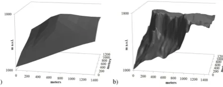
The required smoothing of the MM5 used 200 m DEM as described in Sect. 3 leads to a shift of the apexes and minima when compared to the high resolution 30 m DEM provided by the Nationalpark. These deviations are especially obvious at very exposed areas like Reiteralm (Fig. 2), Watzmann, or Hochkalter. In the case of the Reiteralm the crest of Wart-steinkopf still appears, but as can be seen in Fig. 2 is altered in position and orientation.
Spatial offsets can also be detected when analyzing the wind fields themselves. The topographically caused conver-gence of the airstream and the resulting acceleration of the air masses at the mountains crests are shifted into the faces of the respective massifs when using the 30 m DEM. For the geo-metric correction of the 200 m resolution smoothed DEM and corresponding MM5 wind fields, a polynomial re-sampling approach (Eqs. 2 and 3) with designated control points was applied, using the high resolution Nationalpark 30 m DEM as a reference map:
R0=a1·R2+a2∗C2+a3·R+a4·C+a5·R·C+a6 (2)
C0=b1·R2+b2·C2+b3·R+b4·C+b5·R·C+b6 (3) withR0=new row coordinate,C0 is new column coordinate,
R=old row coordinate,C=old column coordinate,a1−6 and
b1−6=parameters defined over the control points.
The control points are used to generate a (polynomial) transformation that is able to shift the grid elements of the 200 m DEM to the spatially correct location defined by the original 30 m DEM. At least six control points are needed for estimating the coefficientsa1−a6 and b1−b6, which are then also used for correcting all MM5 wind fields.
In the next step, the spatial resolution of the MM5 wind fields was reduced to 30 m by eliminating the coarse grid structure (as evident in Fig. 3a). This was done with a statisti-cal smoothing algorithm and in order to prevent SnowModel predictions from artefacts (edge effects) of the original 200 m resolution. A radial basis function (RBF) (Eq. 4) was used for smoothing of the wind fields while conserving the total amount of energy within each wind field:
φ (r)= −X∞
n=1
(−1)n(σ·r)2n
n!n =ln(σ·r/2) 2+E
1(σ·r/2)2
+CE (4)
Fig. 2. Test site Reiteralm within the smoothed 200 m MM5 DEM (a), and with a original 30 m resolution (b).
with φ (r)=Radial basis function, r=the Euclidean dis-tance (r=||si −s0||) between the prediction location s0 and each data location si, σ=the smoothing parameter, E1=exponential integral function, andCE=Euler constant.
RBF is an exact interpolation technique forcing the new surface through local measurement points. As a result, any 200 m grid element has an identical mean when compared to the average of corresponding newly generated 30 m grid cells.
Fig. 3. (a) Original 200 m MM5 data, (b) smoothed MM5 wind field with a resolution of 30 m, (c) final 30 m MM5 wind field.
the impact of vegetation leads to very small wind speeds in forested regions. This effect becomes obvious in Fig. 3c and can be identified through sharp black edges.
4.2 Validation of downscaled MM5 wind fields
The correlation between measured and modelled daily wind speeds was greatly improved by the downscaling procedure. The original modelled data correlated with anr2 of 0.41 to the measurements while the downscaled set produced anr2
of 0.62 for the season 2003/04 (Fig. 4a, b).
The weak correlation (r2=0.21) of hourly measurements is caused by the general omittance of local and temporary phe-nomena (like cooling or heating of some areas etc.) by the MM5 model, since model runs were initiated with the inten-tion of reaching steady state condiinten-tions for the wind fields under a certain synoptic inflow. The rationale behind this strategy is driven by the assumption that high wind speeds that are generating remarkable snow transport events are pre-dominantly controlled by synoptic inflow rather than local and micrometeorological effects. Summarizing, the determi-nation of the current wind field depends on the synoptic sit-uation which changes less frequently compared to local con-ditions and low correlation of hourly results are therefore in line with expectations.
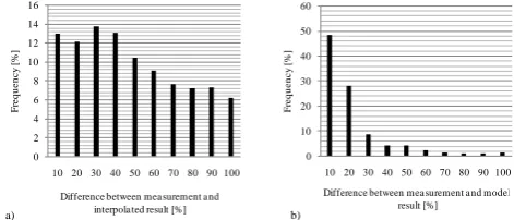
While providing considerably better local wind speed pre-dictions, MM5 generated wind directions are a fundamental improvement in comparison to standard interpolation proce-dures as can be seen for the Reiteralm in Fig. 5, when being evaluated against local measurements. The accuracy (maxi-mum deviation) of the predicted wind directions falls within 10% for about 50% of all measurements (September 2003– August 2004) and within 20% for about 75% (Fig. 5b).
5 Snow transport modelling results
In the following, the performance of the combined Snow-Model – MM5 model is analyzed when predicting horizon-tal snow transport processes at two test sites, Reiteralm and
Fig. 4. (a) Correlation between MM5 results and station recordings
before the downscaling procedure (Reiteralm I, daily resolution).
(b) Correlation between MM5 results and station recordings after
the downscaling procedure. The regression lines are highlighted in black. 0 2 4 6 8 10 12 14 16
10 20 30 40 50 60 70 80 90 100
F re q u e n c y [ % ]
Difference between measurement and interpolated result [%]
0 10 20 30 40 50 60
10 20 30 40 50 60 70 80 90 100
F re q u e n c y [ % ]
Difference between mea surement a nd modell result [%]
a) b)
Fig. 5. (a) Results of interpolated and measured wind directions.
The figure shows that 13% of the interpolation results showing a deviation to the measurements which is less than 10%, 12% are less than 20% and so on. (b) Results of modeled 30 m MM5 data and wind direction measurements. The figure shows that 48% of the model results showing a deviation to the measurements which is less than 10%, 28% are less than 20% and so on. A difference of 100% means that the interpolated wind speed is opposite to the measured one (180◦).
the applicability of the model to a larger range of scales and conditions.
The available satellite images are from April and May 2004 while the field campaign was realized from January 2005 onward. Satellite images of 2005 were not available because the target region was cloud covered for all available dates. Hence, SnowModel runs were performed for the win-ter season 2003/04 and 2004/05 with a temporal resolution of one hour and a spatial resolution of 30 m. The required input parameters, precipitation, humidity, radiation, wind speed, wind direction, air pressure and air temperature were deliv-ered by six meteorological stations (Table 1). The original 10 min data was averaged to hourly values for this study. Reiteralm has an area of about 2 km2and is equipped with 3 meteorological stations. Two of them were installed for observing snow transport activities from the higher situated meteorological station 2, to station 3 (Fig. 1). At K¨uhroint, mainly sheltered from the wind impact, the focus was on cor-rectly reproducing “no transport” conditions.
The parameterization of vegetation classes, decisively controlling the snow holding capacity, was adopted from Lis-ton and Sturm (1998) for the first model run at Reiteralm. After that, a vegetation type “sporadic trees” was created for areas with sparse canopy stands.
5.1 Reiteralm
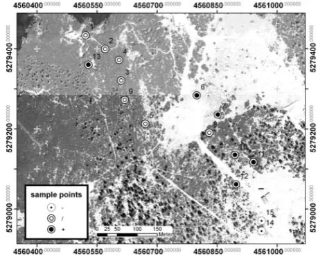
The SnowModel predicted snow depths were generally over-estimated at the upper part of Reiteralm and underover-estimated at the lower parts (see Fig. 6, symbols). A comparison of model and field campaign results reveals that differences be-tween the measurements at the sample points could be repro-duced by the model to some degree, but the modelled vari-ability is generally too small (Table 2).
Table 2 shows the standard deviations (SD) of all measure-ments per date in comparison to SnowModel predicted val-ues. It is obvious that SDs between measurement points are significantly higher than corresponding SnowModel results. Furthermore, the temporal variations of the measured snow depths are also higher, than those of modelled values. The differences within the model results are approximately sim-ilar for the first seven dates and only slightly smaller for the last two dates. Experiences of the Avalanche Warning Ser-vice of Bavaria, observing this site for over 10 years, indicate that considerable amounts of snow are blown from the upper (characterized by sample points 1–8, Fig. 6) to the lower part of the site (sample points 14 and 15, Fig. 6).
This experience is confirmed by the snow depth measure-ments of the automatic meteorological stations Reiteralm II and III but could not be fully reproduced by SnowModel. Horizontal transport processes were underestimated during the first model run using the vegetation class parameterisa-tion of Liston and Sturm (1998), thus a vegetaparameterisa-tion type “spo-radic tree” was created for areas with sparse canopy stands by reducing the snow holding capacity of “deciduous forest”
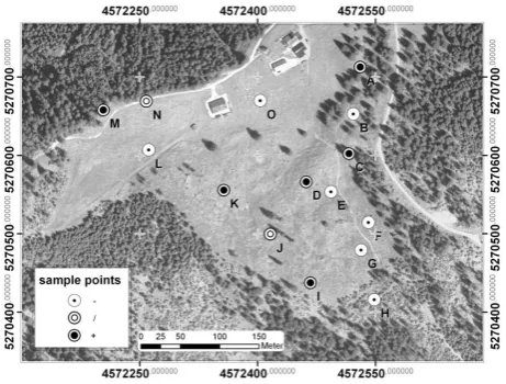
Fig. 6. Test site Reiteralm: the points indicate the position of the
snow gauges. White points with a large black dot in the middle indi-cate that the modelled snow depth of the winter season 2004/05 was in average more than 10% higher than the measured one, whereas white points with a small black point indicate that the modelled snow depth was in average more than 10% below of the measure-ments. White points with a black ring standing for measuring points were the model results are within these thresholds.
to 2 m. By adding the new vegetation type and MM5 wind fields the model results could be improved at the upper part of the Reiteralm (c.p. Fig. 7a), but there were no changes at the lower part (c.p. Fig. 7b, c). When comparing model re-sults using modelled MM5 versus standard interpolated wind fields, differences could be only found at the upper stations (Fig. 7a). Differences at other stations (close to or within the forest) were negligible.
5.2 K ¨uhroint
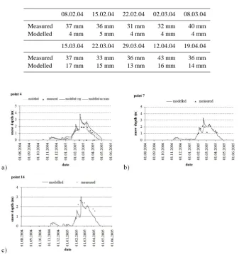
Table 2. Standard deviations of snow depth measurements and of the respective model results for the observation dates (Reiteralm).
08.02.04 15.02.04 23.02.04 02.03.04 10.03.04 14.03.04 23.03.04 30.03.04 05.04.04
Measured 43 mm 41 mm 35 mm 39 mm 54 mm 53 mm 38 mm 37 mm 39 mm Modelled 19 mm 19 mm 21 mm 20 mm 24 mm 23 mm 17 mm 14 mm 12 mm
Table 3. Standard deviations of the snow depth measurements and of the respective model 1 results for the observation dates (K¨uhroint).
08.02.04 15.02.04 22.02.04 02.03.04 08.03.04
Measured 37 mm 36 mm 31 mm 32 mm 40 mm Modelled 4 mm 5 mm 4 mm 4 mm 4 mm
15.03.04 22.03.04 29.03.04 12.04.04 19.04.04
Measured 37 mm 33 mm 36 mm 43 mm 36 mm Modelled 17 mm 15 mm 13 mm 16 mm 14 mm
Fig. 7. SnowModel predicted versus measured snow depths at three representative locations at Reiteralm. (a) is representative for the upper
part of Reiteralm. It shows the difference between the original SnowModel MM5 runs and the runs which used the vegetation class sporadic trees instead of the original parameterisation (characterized by “modelled veg”). (b) A representative result for the central region and (c) for the lower part (c.p. Fig. 6). The introduction of sporadic trees has not modified the results of (b) and (c).
Figure 9 shows three sample points at K¨uhroint. Point N) is located at the edge of the forest at the northern part of K¨uhroint; point F) is located at the clear cut area, and point K) can be found on the meadows in the western part of the area. The three points represent the range of model results of snow depth versus observational data: maximum overesti-mation N), best fit K) and maximum underestioveresti-mation F).
5.3 Comparison of 200 m and 30 m results
Fig. 8. The points indicating the position of the snow gauges. White
points with a large black dot in the middle indicate that the mod-elled snow depth of the winter season 2004/05 was in average more than 10% higher than the measured one, whereas white points with a small black point indicate that the modelled snow depth was in average more than 10% below of the measurements. White points with a black ring standing for measuring points were the model re-sults are within these thresholds.
SWE distribution can be related to altitudinal effects. The remaining variance is due to aspect. Using interpolated wind fields from local measurements at this scale instead, the per-centage related to altitude has increased to 96%, leaving the contribution of aspects negligible (Fig. 10).
The 30 m predictions of SWE are considerably different when compared to 200 m results. Other than in the 200 m model resolution runs, the statistical correlation of elevation and SWE is approximately the same for results with and without MM5 wind fields (MM5: r2=0.93 and MicroMet:
r2=0.94). Figure 10 shows that there is no significant corre-lation between SWE distribution and aspect. The rates of in-dividual snow transport components as illustrated in Fig. 12 on the other hand shows a similar distribution as compared to the 200 m SnowModel/MM5 runs. Considerable transport rates can be observed at crest regions but the spatial extent of the affected areas is smaller for the 30 m results and does not therefore significantly influence the absolute SWE dis-tribution of the area shown in Fig. 11. When comparing to the 200 m MM5 results, the 30 m MM5 transport pattern is more heterogeneous and does not show the clear transport tendency from west to east seen in Fig. 12. For example, transport processes with a south to north component can now be observed at the small crests at the west side of Hochkalter or Watzmann massif which stretch from west to east.
The effect of the sublimation processes within the 200 m and 30 m results can be observed in Fig. 10e and f. The max-imum modelled sublimation rates are slightly higher than those of the 200 m MM5 runs (920 mm to 860 mm) but the total amount of sublimation for the whole area is significantly
smaller (0.5 mm to 12 mm per 30 m grid cell in average). This is due to the fact that areas of high sublimation rates are again limited to the crest regions having a smaller spatial extent in the high resolution DEM. Furthermore, the inten-sity of the saltation and suspension process is higher within the 30 m runs (Fig. 12b and d).
5.4 Case study “Blaueis” glacier
The results achieved for Blaueis glacier have shown that the amount of transported SWE considerably depends on the se-lected model scale and wind simulation method. Principally, it can be stated that the use of SnowModel does not lead to any transport rates from and to the glacier if interpolated wind fields are used. This finding is independent of the used scale. When MM5 wind fields are used on the other hand, significant transport processes can be observed. The Snow-Model 30 m runs in combination with MM5 produce a max-imum SWE gain per pixel of 2140 mm SWE. The average contribution of windblown snow over the total glacier area is 220 mm SWE. The additional amount of SWE corresponds to 12% of the total precipitation (1850 mm) and to 23% of the snowy precipitation (950 mm) within the observed period (03/04) (Fig. 13a).
The 200 m runs in contrast produce considerably differ-ent results. The maximum gain per pixel is greatly reduced (740 mm SWE) and the total average contribution is only 4 mm SWE (Fig. 13b). This can be explained by a scale de-pendent shift – as presented for Reiteralm (Fig. 2a and b) – generating an erosion zone of the glacier located in the crest region of Hochkalter within in the 200 m DEM. Hence, ero-sion prevails and the SWE is reduced compared to the 30 m runs. Figures 13a and b show the wind induced gain and loss of SWE for the Blaueis glacier (30 m vs. 200 m resolution, again), illustrating the problem of an accurate estimation of the location of the accumulation and erosion zones at coarser scales (see Liston, 2004).
5.5 Spatial validation of the 30 m SnowModel-MM5 results
The 30 m SnowModel results are spatially evaluated on the basis of remotely sensed data. Model predictions correspond to the extent and support (Bl¨oschl and Sivapalan, 1995) of Landsat 7 ETM+ images allowing a direct comparison.
Fig. 9. SnowModel predicted versus measured snow depths at three representative locations at K¨uhroint covering the range of model results
of snow depth versus observational data: maximum overestimation N), best fit K) and maximum underestimation F).
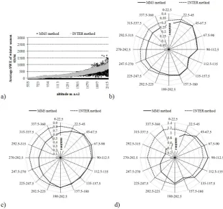
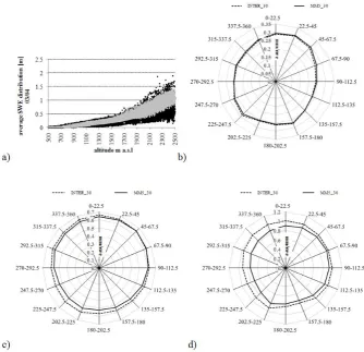
Fig. 10. SnowModel predictions over the winter season 2003/04 at different spatial scales comparing MM5 (MM5 method) generated and
Fig. 11. SnowModel predictions over the winter season 2003/04 comparing 30 m MM5 generated (MM5 method) and interpolated (INTER
method) wind fields. Mean modeled SWE distribution for (a) the total area, (b) areas above 1800 m a.s.l. and (c) areas above 2200 m a.s.l. The different volumes under the curves are due to higher sublimation losses within the MM5 runs.
28 April 2004 (4% on 30 May), while 9% (for both dates) of the modelled grid cells are predicted to be snow covered but are snow free within the classification. The model is overes-timating the extent of the snow coverage on both dates and over the total area. The modelled snow line lies approxi-mately 200–400 m in distance lower than the observed one. It has to be stated that an exact analysis of the model error is difficult due to the fact that the snow line is located in wooded regions on both observation dates.
Another compelling result is that predicted snow cover distributions are much more homogeneous when compared to mapped classification results. While independent of the wind fields used (MM5 or interpolated), it can be attributed to an inability of the model to reproduce the extent of the real transport rates and/or to the fact that the model is not able to handle all transport processes relevant, such as e.g. preferen-tial snow distribution or snow slides.
In order to further analyze SnowModel (30 m) perfor-mance, areas which are snow free within the Landsat 7 ETM+ images, but are predicted to be snow covered were detected in a first step. Then, SnowModel results with and without MM5 wind field integration were compared with a SnowModel run omitting wind induced transport. Using this
run as basis, it is possible to determine to which extent Snow-Model results could be improved by including the blowing snow model algorithm in combination with interpolated wind fields or MM5 wind fields.
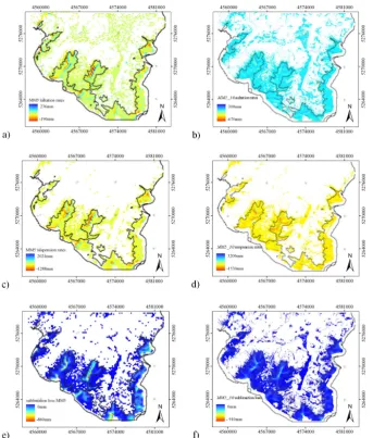
Fig. 12. SnowModel predicted rates of the different transport terms at the 200 m and at the 30 m scale (both with SnowModel and MM5):
saltation, suspension and sublimation in (a), (c) and (e) for 200 m model runs, and (b), (d) and (f) for 30 m model runs with downscaled wind fields. The black line is the 1800 m isohypsis.
Fig. 13. Predicted loss and gain of SWE due to wind induced snow transport at Blaueis glacier (a) 30 m resolution results using MM5 wind
Table 4. Comparison between SnowModel results generated with SnowTran-3D, with and without the usage of MM5. The values belong to
the areas highlighted in Fig. 15a. The areas are snow free in reality, the values within the table showing the improvement of the SnowModel results when the transport routine is used with and without MM5. The percent values standing for the changes of the SWE depth calculated by SnowModel using MM5 or interpolated fields in comparison to SnowModel runs which are omitting snow transport processes.
Improvement when using: Area 1 Area 2 Area 3 Area 4 Area 5 Area 6 Area 7 Area 8 Area 9
Interpolated wind fields 5% 3% 3% 0% 2% 2% −100% 0% −2%
MM5 wind fields 28% 26% 9% 16% 30% 26% 12% 22% 26%
SWE with interpolated wind fields −3 mm −2 mm −1 mm 0 mm −2 mm −2 mm +132 mm 0 mm +2 mm
SWE with MM5 wind fields −18 mm −20 mm −3 mm −18 mm −26 mm −23 mm −16mm −22 mm −21 mm
Table 5. Comparison between SnowModel results generated with SnowTran-3D and with as well as without the usage of MM5. The values
belonging to the areas highlighted in Fig. 15b. The areas are snow free in reality, the values within the table showing the improvement of the SnowModel results when the transport routine is used with and without MM5. The percent values standing for the changes of the SWE depth calculated by SnowModel using MM5 or interpolated fields in comparison to SnowModel runs which are omitting snow transport processes.
Improvement when using: Area 1 Area 2 Area 3 Area 4 Area 5 Area 6
Interpolated wind fields 0% −2 1% 0% 1% 12%
MM5 wind fields 80% 46% 63% 55% 35% 86%
SWE with interpolated wind fields 0 mm +2 mm −1 mm 0 mm −1 mm −2 mm SWE with MM5 wind fields −78 mm −43 mm −39 mm −84 mm −30 mm −31 mm
6 Summary and discussion
The downscaling procedure described in 4 was able to im-prove the convergence between meteorological station and model results in a significant way. The results achieved in Sects. 5.3 and 5.4 are further indicators suggesting the appli-cability of the presented scheme.
The comparison of field campaign data and model re-sults has shown that SnowModel (with or without MM5) is able to reproduce the measured snow depth at Reiteralm and K¨uhroint in a satisfying way (c.p. Figs. 6 and 8). Neverthe-less, the modelled variability between the different measur-ing points was still too small (Tables 2 and 3). Transport pro-cesses from the higher to the lower part of Reiteralm could not be displayed. Further analysis revealed that this is due to the forest which subdivides Reiteralm into two parts. The model treats this forest as a physical barrier which blocks snow transport. The introduction of an additional vegetation class “sporadic trees” resulted in no improvement. This can be attributed to the general model setup. So, a simple reduc-tion of the snow holding capacity makes more snow available for transport but cannot solve the existing lack within the model formulations. For the appropriate representation of snow transport over the forest land cover, two different wind velocity layers would be required within SnowModel, but only one is currently available. While extending SnowTran-3D was bey ond the scope of this project, the required in-put wind fields would in principle be available as from MM5 runs.
The results at K¨uhroint have demonstrated that Snow-Model can reproduce no-transport conditions at a wind shel-tered site in combination with downscaled MM5 wind fields. In correspondence to the results at Reiteralm, the overall variance of the modelled data is too small with respect to the snow depth differences between the sample points. This might be due to the DEM used in this study which describes K¨uhroint, which is undulated in reality, as an almost com-pletely flat area. The DEM at K¨uhroint was checked because of unexpectedly homogeneous snow distribution within the model results. The analysis revealed some inaccuracies within the data, which were unfortunately detected only after the progression of the field campaign. It became evident that the small knolls in the area are not displayed in the DEM even in its original 10 m resolution. However, the example shows that the generation of topographical input parameters can be problematic in Alpine regions and can therefore represent a source for deviations between model and measurements.
Fig. 14. Comparison between SnowModel derived and Landsat 7 ETM+ NDSI classified snow cover distribution (a) NDSI map of 28 April,
2004; (b) NDSI map of 30 May, (c) Modelled snow cover of 28 April, 2004 (200 m resolution) (d) 30 m resolution, (e) Modelled snow cover of 30 May, 2004 (200 m resolution) (f) 30 m resolution. The snow cover is indicated with the blue colour, clouds are masked with the pink colour.
Fig. 15. (a) validation areas of 28 April, 2004: Blue: snow cover, Red: test areas. (Bands: 5,4,3) (b) validation areas of 30 May, 2004: Blue:
of the transported amounts was not possible there. Results presented here indicate that SnowModel-MM5 predictions at the 30 m scale are well able to account for these transported SWE amounts.
The analysis of the general snow cover distribution within the National Park area (Fig. 8) has shown that the effect of wind induced snow transport on the total snow cover distribu-tion is significant at the 200 m scale. However, results at the 30 m scale reveal the importance of wind induced snow trans-port on spatially limited regions, such as the Blaueis glacier or the crest regions of Hochkalter and Watzmann. The ef-fect on the total snow distribution within the National Park is negligible when using the higher model resolution (Fig. 9). This finding is also true for the calculated sublimation rates. The sublimation loss can reach 910 mm within a few pixels at the crest regions. Nevertheless, the influence of the sub-limation process on the water balance for the total region is small within the 30 m results. The average loss by sublima-tion is 0.5 mm per pixel here which is considerably smaller than the 12 millimetres predicted with the 200 m model reso-lution (Fig. 11e and f).
While the integration of 30 m MM5 wind fields can prove SnowModel results in comparison to the satellite im-ages (Tables 4 and 5), SnowModel in combination with in-terpolated wind fields can also reduce the accuracy of the results (Tables 4 and 5). This indicates that the downscaled MM5 wind fields are more reliable – at least in Alpine set-tings – than interpolated wind fields which are the standard setting for the application of SnowModel.
The comparison to the remotely sensed data has also shown that the modelled snow cover is too homogeneous with respect to the mapped snow cover. The inclusion of the 30 m MM5 wind fields has also lead to a more heteroge-neous snow distribution and to an improvement of the spatial SWE distribution (Tables 4 and 5). Nevertheless, the inclu-sion of additional processes like gravitational snow transport or preferential snow deposition would be needed to obtain a more realistic picture of the snow distribution.
As the accuracy of the presented approach is not depen-dent on the general location of the observed area, it could be a helpful alternative for any Alpine environments, indepen-dent on the quality and density of monitoring strategies. Acknowledgements. The authors want to thank the National Park Berchtesgaden authority for providing the GIS information and the meteorological data, as well as the Bavarian Avalanche Warning Service for meteorological data. A special thank goes to the National Park rangers, who accomplished the snow depth measurements; this encouragement of the rangers cannot be ac-knowledged high enough because of the prevailing local conditions.
Edited by: M. Van den Broeke
References
Adrian, G. and Fr¨uhwald, D.: Design der Modellkette GME/LM, PROMET, 27, 106–110, 2002.
Balk, B. and Elder K.: Combining binary decision tree and geo-statistical methods to estimate snow distribution in a mountain watershed, Water Resour. Res., 36, 13–26, 2000.
Bernhardt, M., Z¨angl, G., Liston, G. E., Strasser, U., and Mauser, W.: Using wind fields from a high resolution atmospheric model for simulating snow dynamics in mountainous terrain, Hydrol. Process., 23, 1064–1075, 2009.
Bl¨oschl, G. and Sivapalan, M.: Scale Issues in Hydrological Mod-eling – a Review, Hydrol. Process., 9, 251–290, 1995.
Bowling, L. C., Pomeroy J. W., and Lettenmaier, D. P.: Parameteri-zation of Blowing-Snow Sublimation in a Macroscale Hydrology Model, J. Hydrometeorol., 5, 745–762, 2004.
Bruland, O., Liston, G. E., Vonk, J., Sand, K., and Killingtveit, A.: Modelling the snow distribution at two high arctic sites at Sval-bard, Norway, and at an Alpine site in central Norway, Nordic Hydrology, 35, 191–208, 2004.
D´ery, S. J. and Yau, M. K.: A Bulk Blowing Snow Model, Bound. Lay. Meteorol., 93(2), 237–251, 1999.
Doesken, N. J and Judson, A.: The Snow Booklet: A guide to the science, climatology, and measurement of snow in the United States, Colorado State University, Fort Collins, CO, 1996. Doorschot, J.: Mass transport of drifting snow in high alpine
envi-ronments, online available at: http://e-collection.ethbib.ethz.ch/ show?type=diss\&nr=14515, 2002.
Eidsvik, K. J., Holstad, A., Lie, I., and Utnes, T.: A Prediction Sys-tem for Local Wind Variations in Mountainous Terrain, Bound.-Lay. Meteorol., 112(3), 557–586, 2004.
Essery, R. L. H., Li, L., and Pomeroy, J. W.: A Distributed Model of Blowing Snow over Complex Terrain, Hydrol. Process., 13, 2423–2438, 1999.
Essery, R. L. H.: Spatial statistics of windflow and blowing-snow fluxes over complex terrain, Bound.-Lay. Meteorol., 100, 131– 147, 2001.
Greene, E. M., Liston, G. E., and Pielke, R. A.: Simulation of above treeline snowdrift formation using a numerical snow-transport model, Cold Reg. Sci. Technol., 30, 135–144, 1999.
Grell, G. A., Dudhia, J., and Stauffer, D. R.: A description of the fifth generation Penn State/NCAR mesoscale model (MM5), Technical report, National Centre for Atmospheric Research, Boulder, Colorado, USA, 1995.
Hall, D. K., Riggs, G. A., and Salomonson, V. V.:Development of Methods for Mapping Global Snow Cover Using Moderate Reso-lution Imaging Spectroradiometer Data, Remote Sens. Environ., 54, 127–140, 1995.
Hasholt, B., Liston, G. E., and Knudsen, N. T.: Snow-distribution modelling in the Ammassalik region, south east Greenland, Nordic Hydrology, 34, 1–16, 2003.
Hiemstra, C. A. A., Liston G. E., and Reiners W. A.: Snow redistri-bution by wind and interactions with vegetation at upper treeline in the Medicine Bow Mountains, Wyoming, USA, Arctic Antarc-tic and Alpine Research, 34, 262–273, 2003.
Hiemstra, C. A., Liston, G. E., and Reiners, W. A.: Observing, mod-elling, and validating snow redistribution by wind in a Wyoming upper treeline landscape, Ecol. Modell., 197, 35–51, 2006. Kuhn, M: Zwei Gletscher im Karwendelgebirge, Zeitschrift f¨ur
Kuhn, M.: The mass balance of very small glaciers, Zeitschrift f¨ur Glaziologie und Gletscherkunde, 31, 171–179, 1995.
Lehning, M., Doorschot, J., Raderschall, N., and Bartelt, P.: Com-bining snow drift and SNOWPACK models to estimate snow loading in avalanche slopes, Snow Eng., 4, 113–122, 2000. Lehning, M., V¨olksch, I., Gustafsson, D., Nguyen, T. A., St¨ahli,
M., and Zappa, M.: ALPINE3D: A detailed model of mountain surface processes and its application to snow hydrology, Hydrol. Process., 20, 2111–2128, 2006.
Liston, G. E.: Local Advection of Momentum, Heat, and Moisture during the Melt of Patchy Snow Covers, J. Appl. Meteorol., 34, 1705–1715, 1995.
Liston, G. E. and Sturm, M.: A snow-transport model for complex terrain, J. Glaciol., 44, 498–516, 1998.
Liston, G. E., Winther, J. G., Bruland, O., Elvehoy, H., Sand, K., and Karlof, L.: Snow and blue-ice distribution patterns on the coastal Antarctic Ice Sheet, Antarctic Science, 12, 69–79, 2000. Liston, G. E. and Sturm M.: Winter Precipitation Patterns in
Arc-tic Alaska Determined from a Blowing-Snow Model and Snow-Depth Observations, J. Hydrometeorol., 3, 646–659, 2002. Liston, G. E:. Representing Subgrid Snow Cover Heterogeneities in
Regional and Global Models, J. Climate, 17, 1381–1397, 2004. Liston, G. E. and Elder, K.: A distributed snow-evolution modeling
system (SnowModel), J. Hydrometeorol., 7, 1259–1276, 2006. Plattner, C., Braun, L., and Brenning, A.: The spatial variability
of snow accumulation at Vernagtferner, Austrian Alps, in Winter 2003/2004, Zeitschrift f¨ur Gletscherkunde und Glazialgeologie, 39, 43–57, 2006.
Pomeroy, J. W., Gray, D. M., and Landine, P. G.: The Prairie Blow-ing Snow Model - characteristics, validation, operation, J. Hy-drol., 144, 165–192, 1993.
Pomeroy, J. W., Gray, D. M., Shook, K. R., Toth, B., Essery, R. L. H., Pietroniero, A., and Hedstrom, N.: An evaluation of snow accumulation and ablation for land surface modelling, Hydrol. Process., 12, 2339–2367, 1998.
Prasad, R., Tarboton, D. G., Liston, G. E., Luce, C. H., and Seyfried, M. S.: Testing a blowing snow model against distributed snow measurements at Upper Sheep Creek, Idaho, United States of America, Water Resour. Res., 37, 1341–1356, 2001.
Ryan, B. C.: A mathematical model for diagnosis and prediction of surface winds in mountainous terrain, J. Appl. Meteorol., 16, 571–584, 1977.
Strasser, U., Bernhardt, M., Weber, M., Liston, G. E., and Mauser, W.: Is snow sublimation important in the alpine water balance?, The Cryosphere, 2, 53–66, 2008,
http://www.the-cryosphere-discuss.net/2/53/2008/.
Winstral, A. and Marks, D.: Simulating wind fields and snow re-distribution using terrain-based parameters to model snow accu-mulation and melt over a semi-arid mountain catchment, Hydrol. Process., 16, 3585–3603, 2002.
Z¨angl, G.: An Improved Method for Computing Horizontal Diffu-sion in a Sigma-Coordinate Model and Its Application to Simu-lations over Mountainous Topography, Mon. Weather Rev., 130, 1423–1432, 2002.