www.atmos-meas-tech.net/4/1105/2011/ doi:10.5194/amt-4-1105-2011
© Author(s) 2011. CC Attribution 3.0 License.
Measurement
Techniques
Assimilation of GPS radio occultation data at DWD
H. Anlauf, D. Pingel, and A. Rhodin
Deutscher Wetterdienst, Frankfurter Str. 135, 63067 Offenbach, Germany
Received: 28 January 2011 – Published in Atmos. Meas. Tech. Discuss.: 2 March 2011 Revised: 26 May 2011 – Accepted: 7 June 2011 – Published: 17 June 2011
Abstract. We describe the status of the assimilation of
bend-ing angles from GPS radio occultations in the 3D-Var for DWD’s operational global forecast model GME (“Global Model for Europe”). Experiments show that the assimilation of GPSRO data leads to a significant reduction of biases in the analyses of temperature, humidity and wind in the upper troposphere and the stratosphere, as well as a better r. m. s. fit in the comparison to radiosondes. The impact on forecasts is most prominent in the data sparse Southern Hemisphere, but is also quite notable in the Northern Hemisphere extra-tropics. The positive results found in the impact experiments lead to the implementation of the assimilation of GPS radio occultations from GRACE-A, FORMOSAT-3/COSMIC and GRAS/MetOp-A into the operational suite on 3 August 2010. We also show some initial results from assimilation experi-ments using radio occultation data from the German research satellite TerraSAR-X.
1 Introduction
Data assimilation, i.e., the determination of the state of the at-mosphere from observations plays a central role in numerical weather forecasting. Common observational data sources in-clude in-situ data such as radiosondes, weather station mea-surements, and data from aircrafts and buoys. Nowadays, satellite remote sensing provides an increasing amount of in-formation. Profiles of the thermal structure of the atmosphere can be retrieved from microwave radiance measurements, al-though with vertical resolution less than what is achievable by balloon ascents.
Global Positioning System (GPS) Radio Occulta-tions (RO) (Kursinski et al., 2000) are a relatively new source of observational data with potentially high vertical
Correspondence to: H. Anlauf (harald.anlauf@dwd.de)
resolution (of the order of 100 m). They provide information on temperature and humidity from the atmospheric refrac-tion of the GPS radio signals as measured by a satellite on a low-earth orbit. In contrast to radiance data GPS radio occultations are unaffected by clouds or precipitation and are bias-free (at least at the level of the raw observations). These properties make them interesting in particular for inter-instrument calibration studies, e.g. in climate research. Finally, the horizontal coverage of the radio occultation observations is close to uniform, which is beneficial for their use in data assimilation. Thus, GPSRO data have proven to be a valuable source of information in atmospheric research and weather prediction, and are now being used opera-tionally at many NWP centers, e.g. MetOffice, ECMWF, NCEP, M´et´eo-France, Environment Canada, and JMA (for an overview see the talks and proceedings of the GRAS SAF workshop (2008) and OPAC workshop (2010) and references cited therein).
In the past, the DWD was involved in two projects with focus on the use of GPSRO observations in data assimila-tion. Within the “Radio Occultation Processing Intercompar-ison Campaign” (ROPIC), the processing of initial phase de-lay observations to bending angles with different numerical algorithms, implemented at the participating centres, were compared. At DWD the canonical transform CT2 (see Gor-bunov et al., 2006, and references cited therein) was eval-uated. The results were validated with bending angles cal-culated from the ECMWF model background by a (presum-ably rather accurate) ray-tracing operator based on geometri-cal optics (Gorbunov and Kornblueh, 2003).
DWD, different bending angle forward operators were eval-uated (3-D ray-tracing, 1-D Abel transform, multiple Abel transforms at tangential points of the respective rays) for the use in the 3D-Var data assimilation system of the DWD global model. First impact studies with assimilation of GP-SRO data at DWD (at that time on the IBM RS/6000 Power5 system running under AIX) have shown that these new ob-servations were beneficial for NWP (see Pingel and Rhodin, 2009).
This paper reviews the developments at DWD that lead to the operational use of GPSRO observations in the global numerical weather prediction suite.
2 Assimilation of GPS radio occultations
At the German weather service, the operational assimilation of observational data into the global forecast model GME (Majewski et al., 2002) is performed by a three-dimensional variational assimilation system with a physical space analy-sis scheme (3D-Var PSAS) (Daley and Barker, 2000).
A variational data assimilation scheme determines the analysis by a combination of a preceeding short-range fore-cast (xb) and the observations (yo) with the help of a cost functionJ (x)that contains penalty terms for deviations of the analysis state (x) from both the forecast and the observa-tions, weighted by their respective statistical uncertainties.
J (x) = 1
2 (xb −x)
TB−1(xb −x)
+ 1
2 (yo−H(x))
T R−1(y
o −H(x)) (1)
HereHdenotes the non-linear observation operator, and R and B model the covariances of observation and background error, respectively. The 3D-Var PSAS performs the numeri-cal minimization of the cost function in observation space. The assimilation of radio occultations is performed using bending angles as observations. The model counterpart is calculated from the refractivity field which depends on the atmospheric fields of pressure, temperature and humidity.
The ray-tracing operator (Gorbunov and Kornblueh, 2003) leads to best results in terms of standard deviation of the dif-ference of observation to background (Pingel and Rhodin, 2009) by a small margin, but it has a high computational cost. For the use of GPS radio occultations in operations we cur-rently use a one-dimensional forward operator based on the Abel integral. To take into account the drift of the tangen-tial points relative to the nominal occultation point at least to some extent, an effective occultation point is determined as the mean of the individual rays’ tangential points in the low-est 15 km of the occultation profile.1The refractivity
calcula-1This value is somewhat smaller than the 20 km used in a
pre-vious study (Pingel and Rhodin, 2009). It leads to slightly better agreement between short-range forecasts and observations, proba-bly because the resulting effective occultation point is more
repre-tion uses the expression given in (R¨ueger, 2002) and recom-mended in GRAS SAF Report 05 (GRAS SAF project, 2011) for the neutral atmosphere (see also Healy, 2011 for a criti-cal review and a discussion of non-ideal gas effects which we neglect throughout),
N ≡ 106(n−1) = 77.6890 p
T −6.3938
pw
T
+3.75463 ×10⁵ pw
T2, (2)
whereT denotes the temperature in Kelvin, andpandpw
denote pressure and partial water vapour pressure in hPa. The bending angle,α, for a (locally) spherically symmet-ric atmosphere is a function of impact parameter,a, and can be calculated from the refractive index,n,
α(a) = −2a
Z ∞
a
d lnn/dx
√
x2 −a2 dx, (3)
wherex= nr for vertical coordinater. Above the model top (5 hPa, corresponding to approximately 36 km) the refractiv-ity profile is extended using the MSIS-90 climatology.
The original implementation of Eq. (3) by Gorbunov (Gor-bunov and Kornblueh, 2003) performs the integration using a spline interpolated version of the numerator to a grid reg-ularly spaced in x with a rather small spacing (δx∼50 m) even for high altitudes, which is inefficient. For the opera-tional code which has to run on NEC SX-9 vector processors we performed several adaptations and optimizations, includ-ing a splittinclud-ing-up of the integral into two ranges. The lower part still uses constant integration steps, whereas the upper part uses steps linearly increasing towards the upper integra-tion limit. The numerical integraintegra-tion formula used is exact for a linearly varying numerator in the integrand of Eq. (3) for the lower part. For the upper part we assume an expo-nential variation of the numerator between levels similar to Healy and Th´epaut (2006). In order to keep systematic dif-ferences between the original and modified implementation small in the troposphere and lower stratosphere, the height for the range splitting was set to 30 km.
An error model which accounts for observational errors of each occultation individually, based on the actual situation as provided with COSMIC data or derived by the canonical transform (Gorbunov et al., 2006) should be advantageous. However, in order to use the same model for all data we al-ways applied the error model described in Healy and Th´epaut (2006), where it is assumed that the combination of forward model error and observation error varies only with impact height,h, which is defined ash=a−Rc, whereRcis the ra-dius of curvature provided with the measurement. The stan-dard deviation of the error is assumed to decrease linearly from 10% of the observed value to 1 % for impact heights from 0 to 10 km, and to stay at 1 % above 10 km, with an absolute lower limit of 6×10⁻⁶radians. We do not use the
1e-08 1e-07 1e-06 1e-05 1e-04 1e-03 1e-02 1e-01 1e+00
1e-14 1e-12 1e-10 1e-08 1e-06 1e-04 1e-02 1e+00 1e+02
Normalized difference of gradients
Normalized step size
Comparison of tangent-linear approximation and finite-differences
Fig. 1. Difference of the gradient of the observational cost function for the contribution of a single ray evaluated in the tangent-linear
approximation to finite differencing of the non-linear operator as a function of step size.
observation error provided with the COSMIC data, except when it exceeds the value from the error model. Since we use bending angles for assimilation, we assume that observa-tion errors are vertically uncorrelated.
2.1 Quality control of GPSRO observations
Before assimilation, several checks are applied to the profiles of bending angles:
– As a first step we examine the product quality flag
provided by the processing center. Profiles with non-nominal quality, non-non-nominal processing of excess phase or bending angle will only be monitored.
– For each ray in a profile, we check the consistency of
provided tangent point and georeferencing point, by al-lowing for a maximum great circle distance of currently 3◦, corresponding to a maximum spatial separation of 330 km. In experiments using data before mid-2010 this lead to a rejection of a subset of rays within some COSMIC occultations passing over the 180◦ merid-ian. These occultations typically contained several rays with no reported longitude, and some rays in the pro-file having geographical locations inconsistent with the occultation geometry. This finding was reported to the CDAAC team. The problem was not observed for COS-MIC near real-time data disseminated after 9 July 2010 and appears to have been fixed.
– We exclude occultation events with profiles starting
above 20 km impact height. This mainly affects rising occultations featuring abnormally large first-guess de-partures. (See also Poli et al., 2008, who use a limit of 10 km.)
– An observation-minus-first guess check of 4σis applied
to each ray to remove outliers. This check is chosen less
tight than for conventional observations, as a compensa-tion for a possibly poor representacompensa-tion of the first-guess uncertainty in the upper troposphere and in the strato-sphere, as well as for model bias in the stratosphere. Note that the 3D-Var also employs a variational quality control during minimization that reduces the weight of observations with large departures from the first guess.
– Observations with a relative observation error larger
than 10 % or an absolute observation error larger than 0.01 rad are discarded. This removes observations mostly in the tropical lower troposphere (influence of humidity fluctuations) and in the stratosphere (residual stratospheric fluctuations induce additional noise).
– The value of the bending angle is confined to the interval
[0,0.02] rad to exclude errors due to excessive bending angles (caused by e.g. ducting processes).
– Adjustment of observation errors: To achieve a better
balance in the assimilation process, individual observa-tion errors are adjusted such thateo/ebg>0.5.
– Clipping of the lowest section of GPSRO profiles:
resolution of nonlinearities by radio-optical process-ing can cause a non-monotonous bendprocess-ing angle pro-file. Beneath a given impact height parameter (presently 8000 m) the GPSRO profile section below such points of non-monotonicity is discarded when the bending angle decreases by more than 3 times the assigned observa-tional standard deviation. There is currently no check for the occurrence of super-refraction based on the re-fractivity lapse rate (Poli et al., 2009).
we thin to a vertical spacing of 400 m, between 10 km and 20 km to a vertical spacing of 500 m to 700 m, and between 20 km and 30 km to a vertical spacing of 2 km. The thinning process includes an exponential smoothing of the bending angle profiles in order to remove small-scale fluctuations and to improve the representativity of the observational data. For the assimilation we select impact heights in the range from 3 km to 30 km independent of latitude.
2.2 Monitoring of data and impact experiments
An initial monitoring of GPSRO measurements was per-formed at DWD with near real-time data sets of the CHAMP and GRACE-A missions provided by GFZ, and COSMIC by UCAR (University Corporation for Atmospheric Research) (Pingel and Rhodin, 2009). Impact experiments showed clear benefits of the use of these data. However, the computational cost of the initial implementation was very high, partly due to slow convergence of the 3D-Var when GPSRO were as-similated in addition to other observations, and partly due to the code for the bending angle forward operator needing optimization. The latter issue became even more important when DWD moved the operational system to the NEC SX-9, but it was eventually solved.
The investigation of the slow convergence turned up an inconsistency between the non-linear and tangent-linear/adjoint operator which was finally resolved. The in-consistency was discovered by comparing the gradient of the observational cost function for the contribution of a single ray evaluated in the tangent-linear approximation to finite differencing of the non-linear operator as a function of step size. Figure 1 shows the expected behaviour of the normal-ized difference of the gradients when the increment for finite differencing is chosen as a random vector and the scale of the increment is given by the background error. For large step sizes, the discrepancy is caused by non-linearity of the observation operator, while for very small step sizes round-ing error dominates. The level of the plateau (10−7...10−8) shown in Fig. 1 for moderate step sizes is consistent with the expected accuracy for numerical differentiation with IEEE double precision. For the inaccurate implementation of the tangent-linear operator there was a broad plateau at the level of 10−1...10−2.
Furthermore, we found that convergence was much faster when surface pressure observations were removed from the assimilation. This problem was finally resolved by chang-ing the Variational Quality Control (VQC) for surface pres-sure. VQC is implemented by use of a non-quadratic formu-lation (i.e. a non-Gaussian probability density function) for the observational cost function. In general a Huber-function (Huber, 1973) like expression is chosen which represents a Gaussian p. d. f. with fat tails.2 This formulation was used for all observed quantities except surface pressure, because
2Our formulation consists of a two times differentiable function
which is very similar to the piecewise quadratic or linear Huber
surface pressure observations had a large number of outliers which were not well represented by the fat tails of the Huber p. d. f. but better by a superposition of a Gaussian and a flat distribution. Therefore the latter formulation (see e.g. Ander-sson and J¨arvinen, 1999, and references cited therein) was previously used for surface pressure. The convergence of the minimization was considerably improved when the Huber-function was applied to surface pressure as well.3 We ex-plain the interference of surface pressure observations and radio occultations by the fact that RO basically observe re-fractivity as a function of geometrical height. Rere-fractivity is closely related to atmospheric pressure and therefore RO pro-vide information on pressure as a function of height which otherwise is only constrained by surface pressure observa-tions. All other observation types only provide information on pressure gradients (temperature, thickness).
After the above issues had been addressed, we performed impact experiments for an extended period. These experi-ments exposed several problems in the Antarctic: when com-paring short-range forecasts of both temperature and wind speed to radiosonde observations, we found an increase of the mean departures in the Antarctic stratosphere. In an ex-periment where radio occultations were blacklisted south of 65◦S, these biases clearly decreased to the level of the op-erational system. On the other hand, this increase in bias appeared to have no significant negative impact on other re-gions, so no blacklisting was done when the GPSRO were operationally implemented. Later investigations revealed that part of the increased bias resulted from an inappropri-ate choice of the vertical correlations in the background error covariance model which had been taken over from the previ-ous forecast model resolution.
Furthermore, there is the well-known problem of a nega-tive bias of the bending angles derived from GRAS closed-loop data in the lower troposphere up to about 10 km. In a conservative approach one would blacklist this part of the profiles (Healy, 2008; Poli et al., 2008; Rennie, 2010). On the other hand, according to the error model described above, the assigned observation error for GPSRO observations also increases with penetration into the troposphere, leading to a reduced observation impact.
We performed a comparison of experiments which assim-ilated GRAS data down to 3 km and 8 km impact height, re-spectively. The negative bias in the bending angles appears to lead to a systematic but small reduction of moisture when comparing the respective analyses, but we did not see a sig-nificant detrimental effect in the comparison of short-range forecasts to radiosondes, nor did we see a significant effect
function. The ensuing cost function has a positive definite Hessian and – in absence of strong non-linearities of the observation opera-tor – no multiple minima, leading to enhanced convergence of the minimization algorithm.
3The large number of outliers for surface pressure stems from
-2 -1 0 1 2 Bias of Temperature [K]
925 850 700 500 400 300 250 200 150 100 70 50 30 20
10 0
Area=60/20 0/360 0.0 0.5 1.0 1.5 2.0 2.5 3.0 RMS error of Temperature [K] 925 850 700 500 400 300 250 200 150 100 70 50 30 20
10 0
Pressure (hPa) Pressure (hPa) 8934 19866 23545 24902 24496 24572 24645 24335 23786 23973 23130 21804 20938 19469 17924 9607 -20 -3 4 22 96 59 46 24 54 56 86 55 493 372 1488 1312
-2 -1 0 1 2 Bias of Temperature [K] 925 850 700 500 400 300 250 200 150 100 70 50 30 20
10 0
Area=20/-20 0/360 0.0 0.5 1.0 1.5 2.0 2.5 3.0 RMS error of Temperature [K] 925 850 700 500 400 300 250 200 150 100 70 50 30 20
10 0
Pressure (hPa) Pressure (hPa) 3544 4311 4850 4925 4639 4648 4754 4740 4652 4544 3582 3457 3076 2292 1371 726 -3 -10 -14 38 82 -2 14 2 7 17 541 161 387 -59 70 64
-2 -1 0 1 2 Bias of Temperature [K] 925 850 700 500 400 300 250 200 150 100 70 50 30 20
10 0
Area=-20/-60 0/360 0.0 0.5 1.0 1.5 2.0 2.5 3.0 RMS error of Temperature [K] 925 850 700 500 400 300 250 200 150 100 70 50 30 20
10 0
Pressure (hPa) Pressure (hPa) 1641 2347 2530 2561 2480 2460 2479 2407 2384 2398 2139 2197 1964 1580 732 211 -1 11 13 53 44 50 40 73 85 73 266 93 232 -18 114 11
Fig. 2. The mean departure (left) and RMS difference (right) of radiosonde temperature observations to 3-h forecasts for the reference run
(dash-dotted blue line) and the GPSRO experiment (continuous red line). The rows show the comparisons for observations in the latitude bands 20◦N–60◦N, 20◦S–20◦N, and 60◦S–20◦S (from top to bottom). The central columns display the number of samples used in the experiment (red) and the difference of experiment to reference (black).
in the global precipitation. For this reason we currently apply the same selection and quality control criteria for GRAS as for other GPSRO, but we will reassess these parameters for GRAS when we find evidence for a negative impact.4
4As a side note, we would like to mention that we also
assim-ilate other observations where the presence of a significant bias is established, but their omission would lead to worse forecasts. In the case of aircraft temperature, a bias correction scheme is under development.
2.3 Assimilation results
-10 -5 0 5 10 Bias of Relative Humidity [%]
925
850
700
500
400
300
250
200
Area=-20/-60 0/360 0 5 10 15 20 RMS error of Relative Humidity [%] 925
850
700
500
400
300
250
200
Pressure (hPa) Pressure (hPa) 1666
2273
2158
2127
2262
2216
2183
0
-16
1
-20
24
56
53
17
0
Fig. 3. The mean departure (left) and RMS difference (right) of radiosonde humidity observations to 3-h forecasts for the reference run
(dash-dotted blue line) and the GPSRO experiment (continuous red line) in the Southern Hemisphere (60◦S–20◦S). The central columns refer to the number of used observations, cf. caption of Fig. 2.
0.3 0.4 0.5 0.6 0.7 0.8 0.9 1 1.1 1.2 1.3 1.4
0 24 48 72 96 120 144 168
RMS difference to analysis [K]
Forecast Time [h] Temperature at 50 hPa, NH
GME Routine GMEP GPSRO
0.6 0.8 1 1.2 1.4 1.6 1.8
0 24 48 72 96 120 144 168
RMS difference to analysis [K]
Forecast Time [h] Temperature at 50 hPa, TR GME Routine
GMEP GPSRO
0.5 1 1.5 2 2.5 3 3.5 4
0 24 48 72 96 120 144 168
RMS difference to analysis [K]
Forecast Time [h] Temperature at 50 hPa, SH
GME Routine GMEP GPSRO
Fig. 4. The RMS difference of the 50 hPa temperature as a function of forecast time in the Northern Hemisphere (top), Tropics (middle),
0.4 0.5 0.6 0.7 0.8 0.9 1
0 24 48 72 96 120 144 168
Anomaly correlation
forecast time (h)
ANOC geopotential 500 hPa SH 2010070100 till 2010073100 (31 forecasts)
GME routine GMEP GPSRO
Fig. 5. Anomaly correlation of the 500 hPa geopotential height in
the Southern Hemisphere (90◦S–20◦S) of the reference (GME rou-tine, blue line) and of the GPSRO experiment (red line), based on the statistics from 31 forecasts during July 2010. The shaded blue area and the red error bars indicate the respective 90 % confidence intervals derived from the bootstrap method.
being actively used, with selection criteria as described above and applying the exact data cutoff time of the routine to the GPSRO observations as well.
The set of observations assimilated in the GPSRO ex-periment therefore consisted of in-situ observations from SYNOP stations, BUOYs, SHIPs, aircraft, radio- and drop-sondes, PILOTs, and space-borne remote sensing data in-cluding sea surface winds from ASCAT, atmospheric mo-tion vectors from geostamo-tionary and polar orbiting satellites, AMSU-A brightness temperatures from the MetOp-A and NOAA polar orbiting satellites, and GPSRO bending angles from GRACE-A, FORMOSAT-3/COSMIC 1–6, and GRAS on MetOp-A.
At DWD, the operational global data assimilation system uses a static bias correction scheme for the satellite radiances. The coefficients used in the bias correction are reevaluated off-line from time to time, to counteract drifts of satellite brightness temperature sensors and imperfect model climate. The bias correction is also susceptible to changes that influ-ence the model state in the stratosphere. For the long-term impact experiment using GPS radio occultations, the coef-ficients of the bias correction therefore had to be adjusted independently from the operational system.
Figure 2 shows the comparison of the mean departures (observation minus first-guess) and RMS differences of ra-diosonde temperatures in three latitude bands (20◦N–60◦N, 20◦S–20◦N, and 60◦S–20◦S) for the reference run, which is the operational system, and the GPSRO experiment during July 2010. Evidently the bias and RMS error of the short-range forecasts is reduced, with the impact being largest in the Southern Hemisphere (where less observational data is available than in the Northern Hemisphere) and in the
strato-sphere. A comparison of the count of temperature observa-tions used after variational quality control (displayed in the central columns in Fig. 2) shows that more data are actu-ally used, which can be explained by the better consistency of the short-range forecasts of the GPSRO experiment with radiosonde measurements.
Since the refractivity of air depends on the water vapour pressure (cf. Eq. 2), we should expect some improvement in the comparison to radiosonde humidity observations. Disap-pointingly, this effect is rather small in the Northern Hemi-sphere and in the Tropics. We do find a significant positive effect in the Southern Hemisphere, see Fig. 3. Note, however, that it is restricted mostly to the upper troposphere where the humidity contribution to refractivity is expected to be rather small. We therefore think that this improvement is an indirect effect of the general improvement of the short-range forecast with respect to vertical structure rather than a direct effect of the analysis.
In order to assess the persistence of the information gained by the assimilation of radio occultations, we performed com-parisons of forecasts to each experiment’s own analyses. Fig-ure 4 shows the average RMS difference of the 50 hPa tem-perature as a function of forecast time for the Northern Hemi-sphere (20◦N–90◦N), Tropics, and Southern Hemisphere (90◦S–20◦S) for July 2010. Evidently there is a large re-duction in RMS error in the GPSRO experiment which sig-nificantly increases with forecast lead time. However, some-times there is a minor degradation at shorter forecast lead times, as can be seen from the 12 h forecast time data points for the Northern and Southern Hemispheres. We find this behaviour for temperature forecast also at other stratospheric levels. As a possible explanation for this phenomenon we suggest that the analysis state is either not well balanced or not consistent with the forecast model’s climate.
The impact on forecast quality may be demonstrated by showing the improvement of the anomaly correlation score of the 500 hPa geopotential. For the Northern Hemisphere this impact was rather small, but we found a very nice increase of this score for the Southern Hemisphere, cf. Fig. 5.
As the overall assessment of the impact of GPS radio oc-cultations on forecasts was positive, it was decided to switch on their assimilation into the operational system on 3 Au-gust 2010.
2.4 Radio occultation data from TerraSAR-X
The German research satellite mission TerraSAR-X carries as a secondary payload an IGOR GPS receiver (Beyerle et al., 2010), which is of the same type as those installed on the COSMIC micro-satellites. TerraSAR-X is capable of provid-ing roughly 200 settprovid-ing occultations per day, which are pro-cessed by GFZ Potsdam and disseminated via GTS through DWD since 21 October 2010.
-0.04 -0.02 0.00 0.02 0.04 Bias of (O-B)/O
1
2
3
4
5
6
7
8
9
10
11
12
13
14
15
16
17
18
19
20
21
22
23
24
25
26
27
28
29
30Area=90/-90 0/360 Solid=OBS-FG, Dashed=OBS-AN 0.00 0.02 0.04 0.06 0.08 0.10 Stdev of (O-B)/O 1
2
3
4
5
6
7
8
9
10
11
12
13
14
15
16
17
18
19
20
21
22
23
24
25
26
27
28
29
30
Impact height (km) Impact height (km) 0
0
0
3632
5540
9577
7799
14155
10566
15763
9921
10220
10428
10581
10722
10654
5156
5178
10044
4926
5180
0
4942
0
4707
0
4761
55
5188
47
0
0
0
7128
8891
14524
10220
16930
11602
17080
10981
11095
11040
11147
11192
8782
7724
5465
10649
5140
5564
11
5270
3
5058
2
4891
4
5567
1
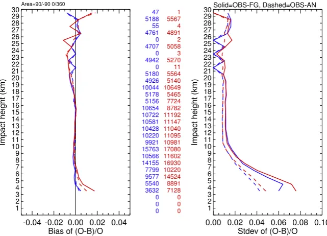
Fig. 6. The global mean (left) and standard deviation (right) of observation minus first-guess (continuous lines) and observation minus
analysis (dashed lines) of the TerraSAR-X (blue) bending angle departures for impact heights from 3 km to 30 km, and compared to COSMIC FM-1 (red). The departures are normalized with respect to the observed bending angles. The statistics is based on 28 days of data (22 October to 18 November 2010). The central columns display the number of samples passing first-guess checks and being used after the variational quality control within a 1-km interval (left: TerraSAR-X, right: COSMIC). Impact heights between 21–22 km, 23–24 km, and 25–26 km were sparsely populated after vertical thinning.
0.5 1 1.5 2 2.5 3 3.5 4 4.5 5
0 24 48 72 96
RMS difference to analysis [hPa]
Forecast Time [h] Mean-Sea-Level Pressure, NH
GME Routine TSR-X Experiment
Fig. 7. The RMS difference of mean-sea-level pressure as a function of forecast time in the Northern Hemisphere for the operational routine
(dashed blue line) and the experiment including GPSRO data from TerraSAR-X (thick red line). The statistics is based on 56 forecasts (00Z and 12Z) corresponding to 28 days of data (22 October–18 November 2010). The error bars give a rough indication of the uncertainty of the mean as estimated from the time series of the RMS differences. The comparisons are performed against each experiment’s own analyses.
to those used in the operational suite. Figure 6 compares the global mean and standard deviation of the first-guess depar-tures and of the analysis depardepar-tures of the bending angles from TerraSAR-X and COSMIC FM-1 for the period from 22 October to 18 November 2010. Taking into account that the TerraSAR-X occultations generally have a smaller pen-etration into the lower troposphere than COSMIC, we
available radio occultation observations. Nevertheless, since we found no negative impact, and since the number of oc-cultations observed by the COSMIC mission is expected to decrease due to its end-of-life approaching, it was decided to switch on operational assimilation of TerraSAR-X data into the 3D-Var on 9 December 2010. At the same time, modified vertical background error correlations were activated to mit-igate the problems encountered in the Antarctic stratosphere (see Sect. 2.2).
3 Conclusions
The above results demonstrate that GPS radio occultations provide valuable information for numerical weather predic-tion, and that their assimilation leads to improved atmo-spheric analyses and forecasts, confirming the findings of other operational weather services. Being a source of in-formation independent of and complementary to previously used data, they may help to detect problems and identify deficits in the data assimilation system.
Experiments using radio occultation data from GRACE-A, COSMIC, and GRAS showed a significant positive im-pact on DWD’s global forecast system, so that assimilation of these data was turned on 3 August 2010. Evaluation of the quality of GPSRO data from TerraSAR-X data was positive, although the additional impact was very small. In light of the already diminishing number of data from the COSMIC mis-sion, and in order to be able to gain the most benefit from this kind of observational data, the assimilation of TerraSAR-X at DWD was activated on 9 December 2010.
Acknowledgements. We thank EUMETSAT and the GRAS SAF
for providing MetOp GRAS data, TACC and UCAR for providing data from the joint Taiwan/U.S. FORMOSAT-3/COSMIC mission, and GFZ for their efforts to provide GPSRO measurements from GRACE-A and TerraSAR-X in near real-time.
Edited by: A. K. Steiner
References
Andersson, E. and J¨arvinen, H.: Variational quality control, Q. J. Roy. Meteor. Soc., 125, 697–722, 1999.
Beyerle, G., Grunwaldt, L., Heise, S., K¨ohler, W., K¨onig, R., Michalak, G., Rothacher, M., Schmidt, T., Wickert, J., Ta-pley, B. D., and Giesinger, B.: First results from the GPS atmosphere sounding experiment TOR aboard the TerraSAR-X satellite, Atmos. Chem. Phys. Discuss., 10, 28821–28857, doi:10.5194/acpd-10-28821-2010, 2010.
Daley, R. and Barker, E.: NAVDAS Source Book 2000: NRL Atmo-spheric Variational Data Assimilation System, Naval Research Laboratory, Monterey, California, 2000.
Gorbunov, M. E. and Kornblueh, L.: Principles of variational assim-ilation of GNSS radio occultation data, Report 350, Max-Planck-Institut f¨ur Meteorologie, Hamburg, Germany, 2003.
Gorbunov, M. E., Lauritsen, K. B., Rhodin, A., Tomassini, M., and Kornblueh, L.: Radio holographic filtering, error estimation, and
quality control of radio occultation data, J. Geophys. Res., 111, D10105, doi:10.1029/2005JD006427, 2006.
GRAS SAF project home page: http://www.grassaf.org/, last ac-cess: 28 January, 2011.
GRAS SAF Workshop on Applications of GPSRO measurements, ECMWF, Reading, UK, 16–18 June 2008, 2008.
Healy, S. B.: Assimilation of GPS radio occultation measurements at ECMWF, in: Proceedings of the GRAS SAF Workshop on Applications of GPSRO measurements, ECMWF, Reading, UK, 16–18 June 2008, 99–109, 2008.
Healy, S. B.: Refractivity coefficients used in the assimilation of GPS radio occultation measurements, J. Geophys. Res., 116, D01106, doi:10.1029/2010JD014013, 2011.
Healy, S. B. and Th´epaut, J. N.: Assimilation experiments with CHAMP GPS radio occultation measurements, Q. J. Roy. Me-teor. Soc., 132, 605–623, 2006.
Huber, P. J.: Robust Regression: Asymptotics, Conjectures and Monte Carlo, Ann. Stat., 1, 799–821, 1973.
Kursinski, E. R., Haji, G. A., Leroy, S. S., and Herman, B.: The GPS Radio Occultation Technique, Terr. Atmos. Ocean. Sci., 11, 53–114, 2000.
Majewski, D., Liermann, D., Prohl, P., Ritter, B., Hanisch, T., Paul, G., Wergen, W., and Baumgardner, J.: The Operational Global Icosahedral-Hexagonal Gridpoint Model GME: Description and High-Resolution Tests, Mon. Weather Rev., 130, 319–338, 2002. OPAC2010: International Workshop on Occultations for Probing Atmosphere and Climate, Graz, Austria, 6–11 September 2010, 2010.
Pingel, D. and Rhodin, A.: Assimilation of Radio Occultation Data in the Global Meteorological Model GME of the German Weather Service, in: New Horizons in Occultation Research, Studies in Atmosphere and Climate, edited by: Steiner, A., Pirscher, B., Foelsche, U., and Kirchengast, G., Springer-Verlag, Berlin, Heidelberg, 111–129, doi:10.1007/978-3-642-00321-9, 2009.
Poli, P., Beyerle, G., Schmidt, T., and Wickert, J.: Assimilation of GPS radio occultation measurements at M´et´eo-France, in: Pro-ceedings of the GRAS SAF Workshop on Applications of GP-SRO measurements, ECMWF, Reading, UK, 16–18 June 2008, 73–82, 2008.
Poli, P., Moll, P., Puech, D., Rabier, F., and Healy, S.: Quality control, error analysis, and impact assessment of FORMOSAT-3/COSMIC in numerical weather prediction, Terr. Atmos. Ocean. Sci., 20, 101–113, 2009.
Rennie, M. P.: The impact of GPS radio occultation assimila-tion at the Met Office, Q. J. Roy. Meteor. Soc., 136, 116–131, doi:10.1002/qj.521, 2010.