R E S E A R C H
Open Access
Probabilistic Volcanic Ash Hazard Analysis
(PVAHA) I: development of the VAPAH tool
for emulating multi-scale volcanic ash fall
analysis
A. N. Bear-Crozier
1*, V. Miller
1, V. Newey
1, N. Horspool
1,2and R. Weber
1Abstract
Significant advances have been made in recent years in probabilistic analysis of geological hazards. Analyses of this kind are concerned with producing estimates of the probability of occurrence of a hazard at a site given the location, magnitude, and frequency of hazardous events around that site; in particular Probabilistic Seismic Hazard Analysis (PSHA). PSHA is a method for assessing and expressing the probability of earthquake hazard for a site of interest, at multiple spatial scales, in terms of probability of exceeding certain ground motion intensities. Probabilistic methods for multi-scale volcanic ash hazard assessment are less developed. The modelling framework presented here, Probabilistic Volcanic Ash Hazard Analysis (PVAHA), adapts the seismologically based PSHA technique for volcanic ash. PVAHA considers a magnitude-frequency distribution of eruptions and associated volcanic ash load attenuation relationships and integrates across all possible events to arrive at an annual exceedance probability for each site across a region of interest. The development and implementation of the Volcanic Ash Probabilistic Assessment tool for Hazard (VAPAH), as a mechanism for facilitating multi-scale PVAHA, is also introduced. VAPAH outputs are aggregated to generate maps that visualise the expected volcanic ash hazard for sites across a region at timeframes of interest and disaggregated to determine the causal factors which dominate volcanic ash hazard at individual sites. VAPAH can be used to identify priority areas for more detailed PVAHA or local scale ash dispersal modelling that can be used to inform disaster risk reduction efforts.
Keywords:Probabilistic, Volcanic ash, Statistical emulator, Hazard, Computational modelling
Background
Numerous approaches have been adopted in the past to assess volcanic ash hazard at the local-scale (10s km) in-cluding observational, statistical, deterministic and prob-abilistic techniques (Bonadonna et al. 2002a; Bonadonna et al. 2002b; Blong 2003; Bonadonna and Houghton 2005; Costa et al. 2006; Magill et al. 2006; Jenkins et al. 2008; Costa et al. 2009; Folch et al. 2009; Folch and Sulpizio 2010; Simpson et al. 2011; Bear-Crozier et al. 2012; Jenkins et al. 2012a; Jenkins et al. 2012b). However, incom-plete historical data on the magnitude and frequency of eruptions worldwide and the difficulties associated with up-scaling computationally intensive volcanic ash dispersal
models have limited regional or global scale assessments (100 s km).
Simple assessments of volcanic ash hazard are based on compiling observations of the distribution of volcanic ash from historical eruptions, an approach that is still adopted worldwide (McKee et al. 1985; Barberi et al. 1990; Bonadonna et al. 1998; Costa et al. 2009). These maps discriminate land areas buried by volcanic ash fall-out in the past from those that have not. Deterministic methods extend the usefulness of observational methods by utilising the benefits of numerical and computational models and typically consider the causes driving the haz-ard. The advantage of this approach is that it is compu-tationally straightforward and provides a conservative result, which can be used to maximise safety. The disad-vantage is that subjective and implicit assumptions made * Correspondence:[email protected]
1Geoscience Australia, GPO Box 378, Canberra, ACT 2601, Australia
Full list of author information is available at the end of the article
on the probability of the chosen scenario commonly re-sult in an overestimation of conservative hazard values, whereby the largest possible eruption may be possible but highly unlikely.
Probabilistic methods estimate the probability of occur-rence of the hazard at a site according to the location, magnitude and frequency of occurrence of hazardous events around that site. They are flexible and can take into account as much data as you have available. Probabilistic methods produce hazard curves, which provide informa-tion on the level of expected hazard for any given time-frame. Incorporating occurrence rate information into hazard analysis is more complex than deterministic, statis-tical or observational approaches. However, the resulting hazard curve is more useful for prioritising regions where more detailed analysis is needed. Probabilistic approaches to volcanic ash hazard assessment are the focus of this study.
Previous work
In the past, probabilistic analyses of volcanic ash haz-ard have focused on quantitative assessments of the frequency and potential consequences of eruptions. Simpson et al. (2011) undertook a quantitative assess-ment of volcanic ash hazard across the Asia-Pacific re-gion using the Smithsonian Institution’s Global Volcanism Program (GVP) database that enabled the straightforward production of magnitude–frequency plots for each country and, to some extent, provinces within countries, in the region. Quantitative ap-proaches have focused on a single source or site of interest at the local scale (10s of km) using tephra dis-persal models (e.g. Campi Flegrei, Italy (Costa et al. 2009); Gunung Gede, Indonesia (Bear-Crozier et al. 2012); Okataina, New Zealand (Jenkins et al. 2008); Somma-Vesuvio, Italy (Folch and Sulpizio 2010) and Tarawera, New Zealand (Bonadonna and Houghton 2005). Numerical simulations of volcanic ash fallout generally involve running a deterministic eruptive sce-nario that represents the most likely event (based on historical investigation and/or modern analogues) over a period of time sufficiently large as to capture all possible meteorological conditions (Magill et al. 2006; Folch et al. 2008a; Folch et al. 2008b; Folch and Sulpizio 2010; Bear-Crozier et al. 2012)
Regional-scale probabilistic volcanic ash hazard assess-ments are less common (Yokoyama et al. 1984; Hoblitt et al. 1987; Hurst 1994; Hurst and Turner 1999; Magill et al. 2006; Ewert 2007). (Jenkins et al. 2012a; Jenkins et al. 2012b) employed a stochastic simulation technique that up-scales implementation of the ash dispersal model ASHFALL for regional-scale assessments (Hurst 1994; Hurst and Turner 1999). This approach presented a method for assessing regional-scale ash fall hazard,
which had not been attempted previously and represents an important step forward in the development of tech-niques of this kind. However, limitations associated with up scaling conventional ash dispersal modelling methods include the computationally intensive nature of regional-scale applications that would require significant high-performance computing resources, long simulation times and could potentially constrain the spatial reso-lution, geographic extent and number of sources consid-ered. Hazard curves of annual exceedance probability versus volcanic ash hazard for individual sites of interest are typically not generated and therefore disaggregating the dominant contribution to the hazard at particular sites of interest by magnitude, source or distance is not captured.
Motivation for the current work
Workers in other geohazards fields (earthquake, wind, flood etc.) have faced similar limitations associated with quantifying hazard on the regional-scale. Major develop-ments were made by seismologists working in this space in the 1960’s, with a view to assessing ground motion haz-ard at multiple sites associated with potential earthquake activity (Cornell 1968). A methodology was developed for quantifying earthquake hazard at the regional-scale named Probabilistic Seismic Hazard Analysis (PSHA; Cornell 1968; McGuire 1995, 2008). PSHA consists of a four-step framework for which uncertainty in size, location and like-lihood of plausible earthquakes can be incorporated to model the potential impact of future events (Robinson et al. 2006). This methodology has since been adapted for tsunami (Lin and Tung 1982; Rikitake and Aida 1988; Geist and Parsons 2006; Thio et al. 2007; Thomas and Burbidge 2009; Sørensen et al. 2012; Power et al. 2013) and applied to regional–scale tsunami hazard assessments (e.g. Indonesia; Horspool et al. 2014). Early attempts at partially adapting PSHA to volcanic ash (on a local scale) were reported by Stirling and Wilson (2002) for two vol-canic complexes on the North Island of New Zealand (Okataina and Taupo). This study seeks to further advance the adaptation of PSHA for volcanic ash hazard at re-gional spatial scales.
Probabilistic Seismic Hazard Assessment (PSHA)
PSHA was developed to assess seismic risk at individual sites however over time the methodology was applied systematically to a grid of points yielding a regional seis-mic probability map with contours of maximum ground motion of equal timeframe (Cornell 1968; McGuire 1995). Traditional PSHA considers the contribution of magnitude and distance to the hazard and selects the most likely combination of these to accurately replicate the uniform hazard spectrum (McGuire 1995). Advances in seismic hazard analysis and the proliferation of high-performance computing have led to the development of event-based PSHA. Event-based Probabilistic Seismic Hazard Analysis allows calculation of ground-motion fields from stochastic event sets.
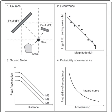
The four-step procedure for event-based PSHA re-ported by Musson (2000) is summarised below and pre-sented in Fig. 1:
1. Seismicity data for the region of interest must be spatially disaggregated into discrete seismic sources. 2. For each seismic source the seismicity is
characterised with respect to time (i.e. the annual rate of occurrence of different magnitudes).
3. A stochastic event set is developed which represents the potential realisation of seismicity over time and a realisation of the geographic distribution of ground motion is computed for each event (taking into account the aleatory uncertainties in the ground motion model).
4. This database of ground-motion fields, representative of the possible shaking scenarios that the investigated area can experience over a user-specified time span, are used to compute the corresponding hazard curve for each site. Hazard curves are computed for each event individually and aggregated to form probabilistic estimates.
This paper presents a methodology developed at Geo-science Australia, which modifies the four-step proced-ure of PSHA for volcanic ash hazard analysis at a regional-scale. The framework named here, Probabilistic Volcanic Ash Hazard Analysis (PVAHA) considers the magnitude-frequency distribution of eruptions and asso-ciated volcanic ash load attenuation relationships and produces an integrated description of volcanic ash haz-ard for all events across a region of interest. An algo-rithm was developed to facilitate a PVAHA named here, the Volcanic Ash Probabilistic Assessment tool for Hazard (VAPAH). This approach builds on the previous work of Stirling and Wilson (2002), Simpson et al. (2011) and Jenkins et al. (2012a; 2012b) towards the development of tools and techniques for conducting regional-scale prob-abilistic volcanic ash hazard assessment.
An assessment for the Asia-Pacific region was under-taken during the development of the VAPAH algorithm. The reader is referred to the companion paper (Miller et al. 2016) for a detailed workflow and discussion of the Asia-Pacific region case study. This paper focuses on the adaptation of PSHA for volcanic ash, the development of the PVAHA framework and the VAPAH algorithm it-self. Results from sub-regions of the Asia-Pacific study are only included here as needed to illustrate concepts and to describe the advantages and disadvantages of the overall approach. This manuscript is divided into four sections:
1. A description of the proposed framework for PVAHA.
2. The procedure used for identification of source volcanoes, development of eruption statistics and calculation of magnitude frequency relationships for each source.
3. Derivation and validation of ash load prediction equations derived from volcanic ash dispersal modelling used to inform the PVAHA. 4. Development of the VAPAH algorithm.
Methodology
A framework for Probabilistic Volcanic Ash Hazard Analysis (PVAHA)
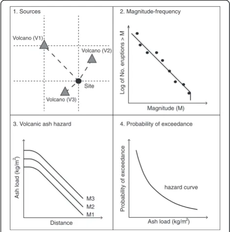
A probabilistic framework for assessing volcanic ash hazard at multiple spatial scales (PVAHA) adapted from Fault (F1)
Site
1. Sources 2. Recurrence
3. Ground Motion 4. Probability of exceedance Area
Fault (F2)
Log of No. earthquakes > M
Magnitude (M)
Peak Accelaration
Distance
Probability of exceedance
Acceleration M1
M3 M2
hazard curve
PSHA is presented here (Fig. 2). The modified four-step procedure is outlined below:
1. Volcanic sources with respect to any given site of interest must be identified.
2. For each volcanic source the annual eruption probability must be calculated based on magnitude-frequency relationships of past events.
3. For a set of stochastic events (synthetic catalogue) volcanic ash load attenuation relationships must be calculated (derived from conventional ash dispersal modelling).
4. Calculation of the annual exceedance probability versus volcanic ash hazard for each stochastic event at each site across a region of interest.
Database development and data completeness
Following the procedure analogous to Jenkins et al. (2012a) a database of volcanic sources and events for the region of interest was prepared using entries from the GVP catalogue. The Smithsonian Institution’s Global Volcanism Program (GVP) catalogue of Holocene events was used to identify volcanic sources for analysis (Siebert et al. 2010). The GVP reports on current eruptions from active volcanoes around the world and maintains a data-base repository on historical eruptions over the past 10,000 years. We acknowledge this database is not a complete record and does contain gaps in the eruption record. Factors that contribute to these gaps, particularly
in data-sparse regions like the Asia-Pacific include incom-plete or non-existent historical records, poor preservation of deposits or lack of accessibility to geographically remote sources. However, the GVP database is widely recognised as the most complete global resource currently available and represents the authoritative source for information of this kind.
Other sources of data can be used to augment an ana-lysis of this kind including volcano observatory archive data and other databases including but not limited to the Large Magnitude Explosive Volcanic Eruptions data-base (LaMEVE; Crosweller et al. 2012). The procedure for creating a database of volcanic sources and events for a PVAHA is described below using the Asia-Pacific examples to provide context where needed (Miller et al., 2016). Database fields including volcano ID, region, sub-region, volcano type, volcano name, latitude, longitude, eruption year and Volcano Explosivity Index (VEI; New-hall and Self 1982) were captured for each eruption at each volcano in a region of interest. These entries were further examined and volcanic sources classified as sub-marine, hydrothermal, and fumerolic or of unknown type were discarded.
Before calculating magnitude frequency relationships each source in the database, the record must be assessed for completeness (Simpson et al. 2011). The eruption record consists of all known events for each volcano in the database. Different magnitude eruptions have differ-ent time periods for which the record is considered complete, and these periods may vary significantly across a region (Simpson et al. 2011). Additionally, larger erup-tions are better preserved in the record than smaller eruptions and this has important implications for data completeness (Jenkins et al. 2012a). With this in mind, events in the database are grouped into sub-regions de-fined by geographic boundaries already adopted by the GVP catalogue for consistency and further subdivided into magnitude classes, VEI 2–3 for smaller magnitude events and VEI 4–7 for larger magnitude events follow-ing the methodology of Jenkins et al. (2012a). Jenkins et al. (2012a) approach for calculating individual record of completeness for each magnitude class was based on reporting by Simkin and Siebert (1994) who declared smaller magnitude eruptions globally complete from the 1960’s and larger magnitude eruptions globally complete over the last century.
Sources with no assigned VEI but designated caldera ‘C’ or Plinian ‘P’ are allocated to the larger magnitude class as arbitrary VEI 4 events. This does not include all the remaining caldera and Plinian eruptions in the data-base, which were assigned a specific VEI (typically in range VEI 4–7). It’s important to note here that only those events classified ‘C’ or ‘P’ with no assigned VEI were arbitrarily allocated to VEI 4. We acknowledge that Volcano (V1)
Site
1. Sources 2. Magnitude-frequency
3. Volcanic ash hazard 4. Probability of exceedance Volcano (V3)
Volcano (V2)
Log of No. eruptions > M
Magnitude (M)
Ash load (kg/m )
Distance
Probability of exceedance
Ash load (kg/m ) M1
M3 M2
hazard curve
2
2
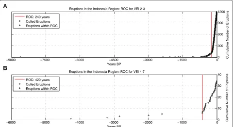
Plinian style, caldera-forming eruptions are commonly associated with eruptions greater than VEI 4 however VEI 4 is selected as a minimum magnitude representing a conservative estimate for the magnitude for the smaller number of these events given the absence of further in-formation (only 13 events identified where this is the case for the Asia-Pacific region). The record of com-pleteness (ROC) was then assessed for each sub-region using the‘break in slope’method by plotting the cumu-lative number of eruptions against time for each magni-tude class for each sub region (Simpson et al. 2011). Similar to Jenkins et al. (2012a) completeness was identi-fied by a linear increase in the cumulative number of eruptions per unit time. The reader is referred to Miller et al. (2016) for the individual ROC values for the Asia-Pacific. An example is provided here for the Indonesia sub-region (Fig. 3).
Magnitude-frequency relationships
Having established the record of completeness for each source in the database a procedure analogous to devel-oping earthquake magnitude-frequency distributions for PSHA is adopted here for assessing the annual rate of occurrence for eruptions of different magnitudes at each source (Musson 2000). Where traditional probabilistic techniques focus on a single volcano for which the haz-ard is estimated independent of the probability of the eruption occurring, the framework reported here is
based on the premise that the ash fall hazard associated with a given site may represent a maximum expected hazard from multiple sources. By extension of this, each source is likely to have varying eruption probabilities, styles and magnitudes and therefore traditional ap-proaches must be modified to accommodate for this heterogeneity (Connor et al. 2001; Bonadonna and Houghton 2005; Jenkins et al. 2008; Jenkins et al. 2012a). In order to calculate the annual eruption probability for each volcanic source at each magnitude the probability of an event of any magnitude occurring and the condi-tional probability of an event of a particular magnitude occurring must be calculated first.
Probability of an event of any magnitude
Firstly, the annual eruption probability for each volcanic source (λ) must be determined by dividing the total number of events (N) by the time period for which the catalogue is thought to be complete (T):
λ ¼ N=T ð1Þ
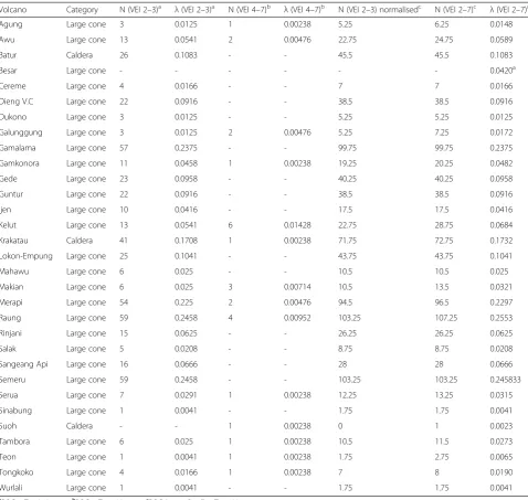
Equation 1 must be solved for each volcanic source in the small and large magnitude classes separately using the associated record of completeness values calculated in the previous section (i.e. λ (VEI 2–3) and λ (VEI 4–7); Table 1). In order to arrive at the likelihood of an event of ‘any magnitude’ occurring (i.e. λ (VEI 2–7) at each
−9000 −7500 −6000 −4500 −3000 −1500 00
300 600 900 1200
Years BP
Cumulative Number of Eruptions
Eruptions in the Indonesia Region: ROC for VEI 2-3
ROC: 240 years Culled Eruptions Eruptions within ROC
−6000 −5000 −4000 −3000 −2000 −1000 00
10 20 30 40
Years BP
Cumulative Number of Eruptions
Eruptions in the Indonesia Region: ROC for VEI 4-7
ROC: 420 years Culled Eruptions Eruptions within ROC
A
B
volcanic source (analogous to PSHA) the total number of events (N) and ROC (T) for each magnitude class in a sub-region must be aggregated into a single value for each. This is achieved by normalising the occurrence interval for the small magnitude class (240 years) to the occurrence interval of the large magnitude class (420 years), with an assumed constant eruption rate. The conversion factor for the number of events is calculated by taking the ratio of the large to the small magnitude completeness periods (e.g. Indonesia; 420:240 = 1.75). The
normalised number of small magnitude events ‘N
(VEI 2–3) normalised’ is then calculated for each source by multiplying the conversion factor (e.g.
Indonesia = 1.75) by the number of small magnitude events ‘N (VEI 2–3; Table 1). The final value for ‘N (VEI 2–7) for each source is calculated by adding the number of small magnitude events ‘N (VEI 2–3) nor-malised’ to the number of large magnitude events ‘N (VEI 4–7; Table 1)’. Sources with no events during the time period for which their record is deemed complete (e.g. Besar) are assigned records from analo-gous volcanoes (those of the same type category) fol-lowing the method of Jenkins et al. (2012a) in order to provide some insight on likely eruption behaviour in the absence of empirical data. Equation 1 can then be solved for the annual eruption probability of each
Table 1Annual eruption probability‘λ(VEI 2–7)’for each volcanic source in the Indonesian sub-region using a conversion factor of 1.75
Volcano Category N (VEI 2–3)a λ(VEI 2–3)a N (VEI 4–7)b λ(VEI 4–7)b N (VEI 2–3) normalisedc N (VEI 2–7)c λ(VEI 2–7)c
Agung Large cone 3 0.0125 1 0.00238 5.25 6.25 0.0148
Awu Large cone 13 0.0541 2 0.00476 22.75 24.75 0.0589
Batur Caldera 26 0.1083 - - 45.5 45.5 0.1083
Besar Large cone - - - 0.0420a
Cereme Large cone 4 0.0166 - - 7 7 0.0166
Dieng V.C Large cone 22 0.0916 - - 38.5 38.5 0.0916
Dukono Large cone 3 0.0125 - - 5.25 5.25 0.0125
Galunggung Large cone 3 0.0125 2 0.00476 5.25 7.25 0.0172
Gamalama Large cone 57 0.2375 - - 99.75 99.75 0.2375
Gamkonora Large cone 11 0.0458 1 0.00238 19.25 20.25 0.0482
Gede Large cone 23 0.0958 - - 40.25 40.25 0.0958
Guntur Large cone 22 0.0916 - - 38.5 38.5 0.0916
Ijen Large cone 10 0.0416 - - 17.5 17.5 0.0416
Kelut Large cone 13 0.0541 6 0.01428 22.75 28.75 0.0684
Krakatau Caldera 41 0.1708 1 0.00238 71.75 72.75 0.1732
Lokon-Empung Large cone 25 0.1041 - - 43.75 43.75 0.1041
Mahawu Large cone 6 0.025 - - 10.5 10.5 0.025
Makian Large cone 6 0.025 3 0.00714 10.5 13.5 0.0321
Merapi Large cone 54 0.225 2 0.00476 94.5 96.5 0.2297
Raung Large cone 59 0.2458 4 0.00952 103.25 107.25 0.2553
Rinjani Large cone 15 0.0625 - - 26.25 26.25 0.0625
Salak Large cone 5 0.0208 - - 8.75 8.75 0.0208
Sangeang Api Large cone 16 0.0666 - - 28 28 0.0666
Semeru Large cone 59 0.2458 - - 103.25 103.25 0.245833
Serua Large cone 7 0.0291 1 0.00238 12.25 13.25 0.0315
Sinabung Large cone 1 0.0041 - - 1.75 1.75 0.0041
Suoh Caldera - - 1 0.00238 0 1 0.0023
Tambora Large cone 6 0.025 1 0.00238 10.5 11.5 0.0273
Teon Large cone 1 0.0041 1 0.00238 1.75 2.75 0.0065
Tongkoko Large cone 4 0.0166 1 0.00238 7 8 0.0190
Wurlali Large cone 1 0.0041 - - 1.75 1.75 0.0041
a
ROC = T = 240 years,b
ROC = T = 420 years,c
source at any magnitude ‘λ(VEI 2–7)’ using the calcu-lated values for ‘N (VEI 2–7)’ and ‘T’ (e.g. Indonesia = 420 years).
Conditional probability of an event of a particular magnitude
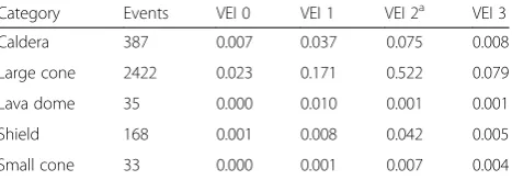
In the previous step, the probability of an event of any magnitude occurring λ(VEI 2–7) at each source was ascertained. The next step is to ascertain the conditional probability of an event being a ‘particular’ magnitude (e.g. VEI 2, 3, 4, 5, 6 or 7). This calculation is performed using the database of events and a classification scheme for volcano morphology (shape) used by Jenkins et al. (2012a). Firstly, all source volcanoes in the database (e.g. Asia-Pacific) are assigned a type category related to their morphology and previous eruption style. Five type cat-egories are considered; lava dome, small cone, large cone, shield and caldera; Table 1). The conditional prob-ability of an event at each magnitude is equal to the number of events for a type category at a particular magnitude divided by the total number of events in the magnitude class (i.e. small magnitude class (VEI 2–3) -Table 2; large magnitude class (VEI 4–7) - Table 3) in the database.
Annual probability of an event
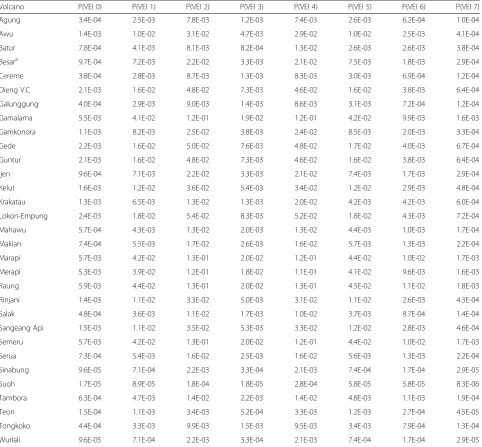
The annual probability of an event of a given magnitude for each source, needed for the PVAHA, can now be cal-culated by multiplying the annual probability of an event of any magnitude for a source by the probability that the event will be a particular magnitude (e.g. Indonesia; Table 4). Metadata is developed to preserve the distinc-tion between annual probability values based on histor-ical data versus analogues (e.g. Besar) so that uncertainty associated with these assumptions is carried through the remaining PVAHA. These magnitude-frequency rela-tionship calculations are repeated for all sub-regions in the database.
Emulating volcanic ash load attenuations relationships Earthquake hazard is measured in terms of the level of ground motion that has a certain probability of being exceeded over a given time period (McGuire 1995, 2008). Ground motion prediction equations (GMPEs) or attenuation relationships are used to provide a means of predicting the level of ground shaking and its associated uncertainty at any given site or location (Fig. 4). GMPEs are based on an earthquake magnitude, source-to-site distance, local soil conditions and fault mechanism and are an integral part of PSHA. A process was developed here for adapting the GMPE approach used for seismic hazard to volcanic ash hazard. The process involves der-ivation of a mathematical expression for volcanic ash load attenuation with distance from source, for an event, using a gridded hazard footprint generated by an ash dispersal model. The resulting equation, named here an Ash Load Prediction Equation (ALPE), statistically emu-lates the volcanic ash attenuation relationship (Fig. 4). Where up scaling of conventional volcanic ash dispersal modelling techniques would be computationally inten-sive and time consuming, ALPEs can be used to emulate generalised volcanic ash hazard (derived from dispersal models) for any given event(s) at any location(s), from any volcanic source of interest as a function of distance of the site from each source.
The procedure for calculating ALPEs for a PVAHA is described below and includes the following:
1. Development of a synthetic catalogue of events 2. Volcanic ash dispersal modelling
3. Derivation of an ALPE 4. Validation of an ALPE
Development of synthetic catalogue of events
Similar to approach taken for PSHA, a synthetic cata-logue of events is developed as a basis for the generation of the ALPEs (one ALPE per event) needed for the PVAHA. A relationship for the rate of volcanic ash load decay with distance from the source, as a function of magnitude, column height, duration, wind turbulence, direction and speed, must be established for each event of interest. The dispersal of volcanic ash through the
Table 2Conditional probability of an event VEI 3 or less occurring for each of the five volcano types in the database (e.g. Asia-Pacific)
Category Events VEI 0 VEI 1 VEI 2a VEI 3
Caldera 387 0.007 0.037 0.075 0.008
Large cone 2422 0.023 0.171 0.522 0.079
Lava dome 35 0.000 0.010 0.001 0.001
Shield 168 0.001 0.008 0.042 0.005
Small cone 33 0.000 0.001 0.007 0.004
a
VEI 2 events in the GVP database are typically more common than VEI 1 and VEI 0 and this is reflected in these values
Table 3Conditional probability of an event VEI 4 or greater occurring for each of the five volcano types in the database (e.g. Asia-Pacific)
Category Events VEI 4 VEI 5 VEI 6 VEI 7
Caldera 49 0.118 0.024 0.024 0.003
Large cone 209 0.500 0.177 0.042 0.007
Lava dome 8 0.017 0.010 0.000 0.000
Shield 18 0.049 0.007 0.007 0.000
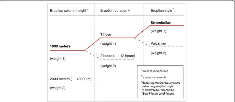
atmosphere produces deposits at ground level that di-minish gradually in load (kg/m2) with distance from the source but in directions controlled by the wind. Consequently, ash load attenuation is a complex func-tion of distance and azimuth from source (Stirling and Wilson 2002). Synthetic events developed here were based on the development of a logic-tree data struc-ture (Fig. 5). The purpose of this strucstruc-ture was to cap-ture all possible variations in volcanological conditions and to quantify the uncertainty associated with the in-puts for each event (Bommer and Scherbaum 2008). The influences of site-specific meteorological condi-tions are considered separately at a later stage in the procedure.
A simplified, schematic representation of the logic tree data structure used is presented in Fig. 5.
Input parameters included:
eruption column height (in meters; between 1 000 and 40 000),
eruption duration (in hours between 1 and 12) and;
eruption style (Strombolian, Vulcanian, Sub-Plinian and Plinian).
A total of 1056 events were developed and assigned an equal weighting for probability of occurrence. Events are not volcano specific but rather represent a suite of synthetic eruptions, which when coupled with
Table 4Annual probability of an event of a particular magnitude occurring for each volcanic source in the Indonesian sub-region
Volcano P(VEI 0) P(VEI 1) P(VEI 2) P(VEI 3) P(VEI 4) P(VEI 5) P(VEI 6) P(VEI 7)
Agung 3.4E-04 2.5E-03 7.8E-03 1.2E-03 7.4E-03 2.6E-03 6.2E-04 1.0E-04
Awu 1.4E-03 1.0E-02 3.1E-02 4.7E-03 2.9E-02 1.0E-02 2.5E-03 4.1E-04
Batur 7.8E-04 4.1E-03 8.1E-03 8.2E-04 1.3E-02 2.6E-03 2.6E-03 3.8E-04
Besara 9.7E-04 7.2E-03 2.2E-02 3.3E-03 2.1E-02 7.5E-03 1.8E-03 2.9E-04
Cereme 3.8E-04 2.8E-03 8.7E-03 1.3E-03 8.3E-03 3.0E-03 6.9E-04 1.2E-04
Dieng V.C 2.1E-03 1.6E-02 4.8E-02 7.3E-03 4.6E-02 1.6E-02 3.8E-03 6.4E-04
Galunggung 4.0E-04 2.9E-03 9.0E-03 1.4E-03 8.6E-03 3.1E-03 7.2E-04 1.2E-04
Gamalama 5.5E-03 4.1E-02 1.2E-01 1.9E-02 1.2E-01 4.2E-02 9.9E-03 1.6E-03
Gamkonora 1.1E-03 8.2E-03 2.5E-02 3.8E-03 2.4E-02 8.5E-03 2.0E-03 3.3E-04
Gede 2.2E-03 1.6E-02 5.0E-02 7.6E-03 4.8E-02 1.7E-02 4.0E-03 6.7E-04
Guntur 2.1E-03 1.6E-02 4.8E-02 7.3E-03 4.6E-02 1.6E-02 3.8E-03 6.4E-04
Ijen 9.6E-04 7.1E-03 2.2E-02 3.3E-03 2.1E-02 7.4E-03 1.7E-03 2.9E-04
Kelut 1.6E-03 1.2E-02 3.6E-02 5.4E-03 3.4E-02 1.2E-02 2.9E-03 4.8E-04
Krakatau 1.3E-03 6.5E-03 1.3E-02 1.3E-03 2.0E-02 4.2E-03 4.2E-03 6.0E-04
Lokon-Empung 2.4E-03 1.8E-02 5.4E-02 8.3E-03 5.2E-02 1.8E-02 4.3E-03 7.2E-04
Mahawu 5.7E-04 4.3E-03 1.3E-02 2.0E-03 1.3E-02 4.4E-03 1.0E-03 1.7E-04
Makian 7.4E-04 5.5E-03 1.7E-02 2.6E-03 1.6E-02 5.7E-03 1.3E-03 2.2E-04
Marapi 5.7E-03 4.2E-02 1.3E-01 2.0E-02 1.2E-01 4.4E-02 1.0E-02 1.7E-03
Merapi 5.3E-03 3.9E-02 1.2E-01 1.8E-02 1.1E-01 4.1E-02 9.6E-03 1.6E-03
Raung 5.9E-03 4.4E-02 1.3E-01 2.0E-02 1.3E-01 4.5E-02 1.1E-02 1.8E-03
Rinjani 1.4E-03 1.1E-02 3.3E-02 5.0E-03 3.1E-02 1.1E-02 2.6E-03 4.3E-04
Salak 4.8E-04 3.6E-03 1.1E-02 1.7E-03 1.0E-02 3.7E-03 8.7E-04 1.4E-04
Sangeang Api 1.5E-03 1.1E-02 3.5E-02 5.3E-03 3.3E-02 1.2E-02 2.8E-03 4.6E-04
Semeru 5.7E-03 4.2E-02 1.3E-01 2.0E-02 1.2E-01 4.4E-02 1.0E-02 1.7E-03
Serua 7.3E-04 5.4E-03 1.6E-02 2.5E-03 1.6E-02 5.6E-03 1.3E-03 2.2E-04
Sinabung 9.6E-05 7.1E-04 2.2E-03 3.3E-04 2.1E-03 7.4E-04 1.7E-04 2.9E-05
Suoh 1.7E-05 8.9E-05 1.8E-04 1.8E-05 2.8E-04 5.8E-05 5.8E-05 8.3E-06
Tambora 6.3E-04 4.7E-03 1.4E-02 2.2E-03 1.4E-02 4.8E-03 1.1E-03 1.9E-04
Teon 1.5E-04 1.1E-03 3.4E-03 5.2E-04 3.3E-03 1.2E-03 2.7E-04 4.5E-05
Tongkoko 4.4E-04 3.3E-03 9.9E-03 1.5E-03 9.5E-03 3.4E-03 7.9E-04 1.3E-04
Wurlali 9.6E-05 7.1E-04 2.2E-03 3.3E-04 2.1E-03 7.4E-04 1.7E-04 2.9E-05
a
magnitude-frequency statistics and prevailing meteoro-logical conditions for a region of interest, can be used to assess a range of potential events at any volcanic source. It is important to note that assignment of weightings can be modified where prevalent eruption behaviour for a region of interest is well known.
Volcanic ash dispersal modelling
The volcanic ash dispersal model FALL3D was used here to computationally model volcanic ash fall hazard footprints needed for the calculation of ALPEs. FALL3D is a time-dependant Eulerian model that solves the ad-vection–diffusion-sedimentation (ADS) equation on a
Bommer et al. (2007) Akkar & Bommer (2007)
M 7.0
6.0
5.0
4.0
M 3.0
w
w
100 10
1
0.1 1
PGA
(cm/s )
2
R distance (km)jb
ALPE 100
VEI 5
VEI 4
VEI 3
10
1
log_volcnaic ash load (kg/m )
2
log_distance (km)
2 10
10 10 10 10
0 2 3 4 5
102 10
3 0
10 10 10
0 2 3
A
B
ALPE 150 ALPE 201
Fig. 4aExample plot of predicted peak ground acceleration with changing distance using two European GMPE’s for different magnitude ranges modified after Akkar and Bommer (2007) and Bommer et al. (2007); (b) Example plot of volcanic ash load attenuation relationships using three ALPEs generated through dispersal modelling for this study (ALPE 100 - VEI 3; ALPE 150 - VEI 4; ALPE 201 - VEI 5)
1000 meters
2000 meters ( . . 40000 m)
Strombolian
Vulcanian 1 hour
2 hours ( . . .12 hours) (weight 1)
(weight 1)
(weight 2)
(weight 1)
(weight 2) Eruption column height * Eruption duration ^ Eruption style
dispersal model parameters reflecting eruption style (Strombolian, Vulcanian, Sub-Plinian andPlinian) 1 hour increments 1000 m increments
o
(weight 2)
structured terrain-following mesh. FALL3D outputs time-dependant deposit load at ground level as a hazard footprint of changing ash load with distance from source (Folch et al. 2012). It is acknowledged that FALL3D is one of a number of suitable ash dispersal models that could be utilised for an analysis of this kind.
An assessment of the mass eruption rate, height and shape of the eruption column is made for each schastic event in the catalogue. These parameters to-gether describe the eruptive source term needed to simulate the dispersal of volcanic ash using FALL3D. The source term can be defined as either a 1-D buoy-ant plume model (Bursik 2001) or as an empirical rela-tionship (Suzuki 1983). The empirical relarela-tionship (Suzuki, 1983) used here estimates the mass eruption rate (MER) given an eruption column height (H) using known best-fit relationships of MER versus H (Sparks et al. 1997). A generalised total grainsize distribution (TGSD) is used to account for a range of eruption po-tential eruption styles which includes minimum and maximum grainsize (phi), average grainsize (phi), sort-ing, density range (kg/cm3) and sphericity of clasts. FALL3D was used to simulate 1056 events in the syn-thetic catalogue.
Derivation of ash load prediction equations
A script was developed for extracting the volcanic ash attenuation relationship (changing ash load with dis-tance) for each hazard footprint generated by the disper-sal model in the synthetic catalogue (Fig. 6). Each ALPE represents a single event (1056 total). When coupled with magnitude-frequency statistics and prevailing
meteorological conditions for a region of interest, each ALPE can be used to statistically emulate the expected volcanic ash hazard from an event of this kind at any lo-cation of interest from any volcanic source as a function of distance of the site from the source. Not unlike GMPEs used to conduct PSHA, the generation and ap-plication of ALPEs will have a considerable influence on the outcome of the PVAHA. The ALPEs developed here use the dispersal model FALL3D however other dispersal models could be used (e.g. ASHFALL (Hurst 1994; Hurst and Turner 1999), HAZMAP (Costa et al. 2009), or TEPHRA (Bonadonna and Houghton 2005)) and the authors would encourage the development of ALPEs using a range of dispersal models currently available to build on and compare/contrast with the current work.
Validation
In order to determine the uncertainty of the ALPEs or the degree to which they accurately reproduce simulated ash fallout generated by FALL3D and observed deposit data gathered from field studies of historical eruptions, a validation is presented for the F2 Plinian fall deposit generated by the 1815 eruption of Tambora, on the is-land of Sumbawa, Indonesia. FALL3D has already been widely validated against several tephra deposits and air-borne ash cloud observations from different eruptions (Costa et al. 2006; Macedonio et al. 2008; Scollo et al. 2008a; Scollo et al. 2008b; Scollo et al. 2009; Corradini et al. 2011; Costa et al. 2012; Kandlbauer et al. 2013; Costa et al. 2014; Kandlbauer and Sparks 2014). An in-version simulation for the Tambora F2 deposit data is
0
0 100 200 300
300 200 100 0
Ash load (kg/m )2
A
distance (km)
distance (km) 100
200
300 300
200
100
300 200 100
(..) d c b a
10
1
log_volcnaic ash load (kg/m )
2
log_distance (km)
2 10
10 10
1 2 3
102 103
1
B
500 400
volcanic ash load attenuation
presented here using FALL3D by comparing observed measurements for the F2 deposit at 27 sample locations with simulated ash measurement generated by FALL3D at all corresponding sample sites (Sigurdsson and Carey, 1989). We then generate an ALPE from the FALL3D data following the methodology outlined above and use this equation to calculate the expected ash fallout for the F2 deposit. We present difference plots to compare ob-served versus simulated (FALL3D), simulated versus cal-culated (ALPE) and calcal-culated versus observed estimates (Sigurdsson and Carey 1989) for volcanic ash load and comment on performance of the ALPE for emulating the Tambora F2 Plinian fall deposit.
Validation of FALL3D for the Tambora F2 Plinian fall deposit
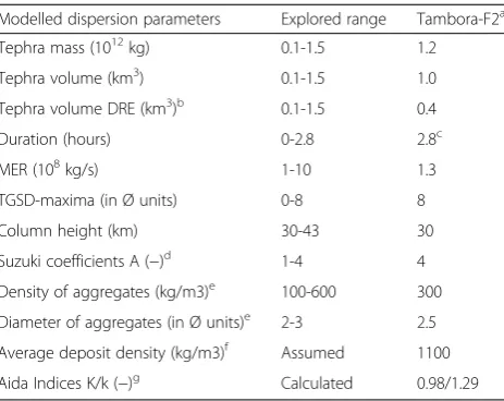
To inverse model the Tambora F2 Plinian fall deposit, the validation method of Costa et al. (2012) is adopted. Costa et al. (2012) constrained the eruption dynamics and ash dispersal characteristics associated with the Campanian Ignimbrite (39 ka) eruption in Italy and later the Youngest Toba Tuff (75 ka) super-eruption in Indonesia. This approach combines tidependant me-teorological fields for the region, a spectrum of volcano-logical parameters (erupted mass, mass eruption rate (MER), column height and total grainsize distribution) and over 100 simulations of the ash dispersal model, FALL3D. Optimal values of the input parameters are ob-tained by best-fitting measured Tambora F2 tephra thicknesses over the entire dispersal area (27 locations) and minimising the deviation of regression. The ex-plored range of input parameters for the Tambora-F2 eruption is reported in Table 5.
Ten years of wind data (January 2000 to December 2010) were obtained from the National Centres for Environmen-tal Protection (NCEP) and Atmospheric Research (NCA) global reanalysis project (Kistler et al. 2001). The NCEP/ NCAR reanalysis data archive contains six hourly data at 17 pressure levels ranging from 1000 to 10 mb with a 2.5° horizontal resolution. The methodology of Costa et al. (2012) used here assumes that this collection of modern meteorological fields can statistically represent a proxy for those at the time of the Tambora F2 eruption (~200 years ago). Vertical meteorological profiles were extracted from the wind data at a gridded location closest to the source and interpolated to the FALL3D computational grid. In order to reduce the computational requirements, vertical, but not horizontal, changes in wind conditions with dis-tance from the source were accounted for here at six hourly intervals using linear temporal and spatial interpolations. The computational domain was discretised by a horizontal grid step ofΔx =Δy = 1.35 km and a vertical step of Δz = 1 km. The computational domain extended from 9° S to 7° N and from 117° E to 118° W.
The distribution of mass within the column was calcu-lated using an empirical parameterisation based on that of Suzuki (1983) and Pfeiffer et al. (2005). In order to ac-count for aggregation processes (clustering of fine ash particles) an aggregation model similar to that of Cornell et al. (1983) and used by Costa et al. (2012; 2014) was adopted here. This aggregation model assumes that 50 % of the 63–44 μm (4–4.5Ø) ash, 75 % of the 44–31 μm (4.5-5Ø) ash and 95 % of the sub-31 μm (<5Ø) ash fell as aggregated particles. The diameter and density of the aggregates were determined by best fit in the simula-tions. An approach developed for best fitting the spatial variation between recorded and simulated tsunami heights, the Aida indices Aida (1978) was adopted by Costa et al. (2014) for tephra and is similarly used here to measure the reliability of modelled results. The Aida index K represents the geometric average of the distribu-tion and the second index k is the associated standard deviation of the distribution:
log K¼1ni¼1nlog Ki ð2Þ
log k ¼ 1nn¼1n log Kið Þ2‐ðlog KÞ2 1=
2
ð3Þ
Table 5The explored range and best-fit input parameters modelled dispersion of the Tambora-F2 fall deposit using FALL3D Modelled dispersion parameters Explored range Tambora-F2a
Tephra mass (1012kg) 0.1-1.5 1.2
Tephra volume (km3) 0.1-1.5 1.0
Tephra volume DRE (km3)b 0.1-1.5 0.4
Duration (hours) 0-2.8 2.8c
MER (108kg/s) 1-10 1.3
TGSD-maxima (in Ø units) 0-8 8
Column height (km) 30-43 30
Suzuki coefficients A (−)d 1-4 4
Density of aggregates (kg/m3)e 100-600 300
Diameter of aggregates (in Ø units)e 2-3 2.5
Average deposit density (kg/m3)f Assumed 1100
Aida Indices K/k (−)g Calculated 0.98/1.29
a
These scenarios are the combination of meteorological and volcanological parameters that best reproduce the observed deposits of the Tambora F2 Plinian fall layer
b
A density value of 2650 kg/m3
(trachyandesite) was used to convert into DRE volume
c
Short eruption duration interpreted to be the result of high magma discharge rate (Sigurdsson and Carey,1989)
d
The eruption source is described in a purely empirical way in order to reproduce the optimal geometrical shape of the deposits using the Suzuki distribution (in this instance the eruption column acts as a vertical line source)
e
Aggregation is accounted for using a model similar to that of Cornell et al. (1983) assuming that 50 % of the 63–44μm (4–4.5Ø) ash, 75 % of the 44–31μm (4.5-5Ø) ash and 95 % of the sub-31μm (<5Ø) ash fell as aggregated particles
f
This density value was used to convert deposit thickness, in mass loading and to calculate total tephra volume
g
where n is the total number of measurements and Ki = Mi/Hi is the ratio of measured thickness (load) at Mi,,the i-the location and Hi is the simulated thickness (load) at the same site. In keeping with the approach for tsunami and Costa et al. (2014) we consider the simulated tephra thickness results satisfactory when:
0:95<K>1:05 and k<1:45
The best-fit results from FALL3D are reported in Table 5 and indicate that the MER was ~1.2 x 10⁸kg/s, the eruption column height was ~33 km and the total mass deposits as fallout was ~ 1.2 x 10¹⁴ kg. These re-sults are in good agreement with estimates made by Si-gurdsson and Carey (1989) based on field observations. The corresponding simulated, best-fit, deposit thick-nesses are depicted in a difference plot and reported in Fig. 7. The correlation coefficient between log (measured thickness) and log (simulated thickness) is 0.87 for the best meteorological fit. All simulated thicknesses are
between 1/5 and 5 times the observed thicknesses and the reliability of the best-fit results are further emphasised by the Aida index values; reflecting a geometric average, K = 0.98 and a geometric standard deviation, k = 1.29.
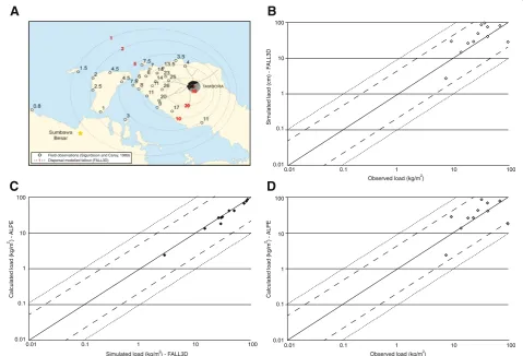
Validation of an ALPE for the Tambora F2 Plinian fall deposit
Following the procedure outlined above the volcanic ash attenuation relationship for the best-fit FALL3D simula-tion was considered and an ALPE was derived for this event. For the purposes of this validation all volcanic ash thicknesses were converted to load (kg/m2) the preferred unit of measurement for PVAHA. Validation of the ALPE was a two-step process involving first, verification that the ALPE could statistically emulate the simulated deposit load generated by FALL3D in previous step and secondly that when compared with the observed data of Sigurdsson and Carey (1989) for this event, ash load values were in good agreement with field measurements at the 27 sample localities. Following the methodology
A
B
C
D
of Costa et al. (2012) the modelled results are considered to be in good agreement with the measured observations when they are between 1/5 and 5 times the observed thickness (Fig. 7). A difference plot indicates good agree-ment (within 1/5 to 5 times), between the simulated best-fit (FALL3D) load (kg/m2) and the observed load (converted from thickness; (Sigurdsson and Carey 1989) plotted here at 27 sample localities (Fig. 7b). To verify that the calculated load from the ALPE closely approxi-mates the simulated load from FALL3D (from which it was derived), a difference plot was generated. As ex-pected, the calculated load and the simulated best-fit load are in good agreement (Fig. 7c). Finally, to complete the validation process the calculated load must be com-pared with the observed field data. A difference plot is generated and the calculated load (ALPES) and the ob-served load are found to be in good agreement (Fig. 7d).
Results
Volcanic Ash Probabilistic Assessment tool for Hazard (VAPAH)
An algorithm was developed to facilitate the fourth step of the PVAHA framework named here, the Volcanic Ash Probabilistic Assessment tool for Hazard (VAPAH). VAPAH utilises a scripted interface and high perform-ance computing technology in order to undertake assessments at multiple spatial scales. The VAPAH algo-rithm reads in magnitude-frequency relationships, an ALPE catalogue and global scale meteorological condi-tions for a region of interest and integrates across all possible events to arrive at a preliminary annual exceed-ance probability for each site across the region of inter-est. Other algorithms of this kind have been developed for probabilistic earthquake hazard assessment (e.g. the Earthquake Risk Model (EQRM; (Robinson et al., 2005) however this algorithm is the first of its kind specifically designed for volcanic ash hazard. Inputs for the VAPAH algorithm include:
1. Identification of volcanic sources for analysis. 2. Characterisation of magnitude-frequency relationships
for each volcanic source.
3. Characterisation of the volcanic ash load attenuation relationship (ALPE catalogue).
4. A spatial grid of pre-determined resolution clipped to the domain extent (default = auto-generated). 5. Characterisation of meteorological conditions
-prevailing wind direction (degrees) and wind speed (m/s)
Identification of volcanic sources, characterisation of magnitude-frequency relationships for each source and development of an ALPE catalogue have all been de-scribed previously. Characterisation of the meteorological
conditions for the region of interest are discussed below using the Indonesian sub-region as an example.
Characterisation of meteorological conditions
The VAPAH algorithm requires an estimation of the prevailing wind direction (degrees) and speed (m/s) at a single pressure level for each source. Meteorological data can be sourced from direct observations (e.g. weather balloons, anemometers and wind vanes) or modelled data available at multiple spatial scales depending on the purpose of the PVAHA (e.g. National Centres for Envir-onmental Protection and Atmospheric Research re-analysis (NCEP/NCAR), Weather Research and Fore-casting Model (WRF) and the Australian Community Climate and Earth System Simulator ACCESS). These estimates for wind direction and wind speed are consid-ered to be highly prevalent at each location by the algo-rithm and are assigned a probability weighting according to a Gaussian distribution with a standard deviation assigned by the user. An example is provided below for the deriving these variables for the Indonesia sub-region using one potential source of meteorological data.
Sixtyfour years of meteorological data (January 1950 -December 2014) was sourced from the NCEP/NCAR re-analysis for the Indonesia sub-region, available at grid inter-vals of 2.5° globally. Among other variables, wind direction and wind speed vector components are available for 17 pressure levels to a height of 40 km. Monthly mean vector components for meridional wind (u-component) and zonal wind (z-component) were extracted at 16 locations across Indonesia, from NCEP grid points closest to each volcanic source at the 250mb pressure level (Tropopause) for a 64 year period (Fig. 8). Monthly mean wind direction (degrees) and wind speed (m/s) were derived from the u and v wind components and aggregated first for each year and then for the 64 year period using the freeware me-teorological analysis and plotting tool, WRPLOT (Table 6). Prevailing wind direction and wind speed were assigned to each source from the closest NCEP point.
VAPAH algorithm procedure
The operational procedure for the VAPAH algorithm is presented in Fig. 9. A configuration file is used to cus-tomise the extent of the assessment (Attachment 1). The configuration file reads in a series of CSV (comma sepa-rated value) files including:
1) the ALPE catalogue,
2) the volcano sources (included prevailing wind speed and direction)
3) the sites of interest (pre-processed spatial grid)
user, geographic coordinates for the region of interest and the resolution can be input for auto-generation of the spatial grid by VAPAH. The user must define the timeframes of interest (e.g. 100, 500, 1000 etc.) in the configuration file. Mean wind direction and mean wind speed for each source are pre-configured (see previous section) however wind direction and wind speed prob-abilities vary seasonally, particularly in equatorial re-gions. The configuration file captures this uncertainty through the wind direction distribution parameter (e.g. normal or bimodal), the wind direction distribution standard deviation parameter (degrees), the wind speed distribution parameter (e.g. normal or bimodal distribu-tion), the wind speed distribution standard deviation parameter (m/s) and the number of wind speeds. Finally, hazard thresholds such as maximum distance from source, maximum ash load value at source and mini-mum sum of ash load needed to generate hazard curves or histograms can be set here by the user.
The VAPAH algorithm can be run in serial or parallel computing environments (i.e. on one or many processors simultaneously) but is optimised for high performance
computing platforms utilising thousands of CPUs. Simula-tion time will vary according to the number of events, the number of sources, the resolution of the hazard grid and the distribution and standard deviation of meteorological conditions. A script is used to execute the procedure as follows:
1. The first site is located on the hazard grid and the distance is calculated in kilometres between this site and the first source in the catalogue.
2. The distance value is used to evaluate the first ALPE for the first synthetic event in the catalogue in order to derive the expected ash load (kg/m2) at that site for the first event.
3. The calculated ash load for the first event and its associated probability derived from the magnitude-frequency relationships for the first source in the catalogue are written to a results file.
4. The algorithm repeats (2) and (3) for each ALPE for the first source.
5. The algorithm then moves to the next source in the catalogue and repeats steps (2), (3) and (4) until all
NCEP point volcanic source
NCEP_0 NCEP_7 NCEP_15 NCEP_12
ALPES have been assessed for the first source for the first site.
6. The algorithm will then calculates the cumulative probability of each event (e.g. each instance where a volcanic ash load was recorded from one or more sources) for the first site and generates a hazard curve of volcanic ash load (kg/m2) versus annual probability of exceedance and the maximum expected ash hazard for timeframes of interest (specified by the user in the configuration file). This process will capture all instances where the first site might experience multiple ash hazards from more than one source.
7. The algorithm then loops to the next site and repeats steps (1)–(6) until all sites have been evaluated.
VAPAH results
VAPAH generates a database file of hazard calculations collectively referred to here as the PVAHA. Like, PSHA the PVAHA results can be post-processed using VAPAH to generate hazard curves for annual probability of ex-ceedance at sites of interest (or all sites), maps for max-imum expected ash hazard at timeframes of interest and histograms which disaggregate the hazard (e.g. location, magnitude, source etc.) for determining the primary causal factors at sites of interest. Examples of each for the Indonesia sub-region are reported in Fig. 10). Hazard curves report the annual exceedance probability versus
volcanic ash load for a site of interest. These curves capture all instances where the site experienced ash loading from events originating from one or more sources (potentially thousands of events) that ash load will exceed a particular value (Fig. 10). The expected maximum ash load for timeframes of interest is also calculated. By aggregating the hazard calculations for each site, hazard maps can be generated which display the maximum expected ash load (kg/m2) at each site across the region for a timeframe of interest (e.g. 1-in-100 year event; Fig. 10). It’s important to clarify that a 1-in-100 year event does not suggest that the max-imum expected ash load for a site will occur regularly every 100 years, or only once in 100 years but rather, given any 100 year period, the maximum expected ash load for a particular site may occur once, twice, more, or not at all.
Disaggregation of the hazard calculations can ascertain which events dominate the hazard at a particular site. The ability to disaggregate the primary causal factors contributing to the hazard at a given site (i.e. magnitude, source, distance, ash load etc.) is an inherent strength of this approach. The user can specify disaggregation pa-rameters in the configuration file prior to undertaking an assessment and the VAPAH algorithm will generate histograms as part of the PVAHA results set (Fig. 10). Alternatively, histograms can be generated using a pre-generated database of events from assessments already computed. This functionality is useful for demonstrating what the percentage contribution to hazard of different volcanic sources on a site located in for example‘Jakarta’ might be, and of those volcanic sources what proportion are VEI 2, 3, 4, 5, 6 and 7 (Fig. 10).
Discussion
The PVAHA methodology presented here integrates across all possible events and expected volcanic ash loads to arrive at a combined probability of exceedance for a site of interest. The analysis incorporates the rela-tive frequencies of occurrence of different events and a wide range of volcanic ash dispersal characteristics. Like PSHA, this quantitative method of estimating volcanic ash hazard has the advantage of providing consistent es-timates of hazard and can be prepared for one site or many, all in the same region but in significantly different geographic orientations with respect to potential hazard sources (McGuire 1995, 2008).
The methodology is highly customisable allowing for the flexible integration of ALPEs generated using numer-ous ash dispersal models and eruption statistics derived from a variety of sources (Whelley et al. 2015). Capacity to build in flexibility in input assumptions highlights the power of this approach for quantifying uncertainty. The VAPAH algorithm effectively replaces the need for
Table 6Monthly mean wind direction and wind speed aggregated for a 64-year period (1950–2014) for 16 NCEP grid points across the Indonesian sub-region
NCEP point Longitude Latitude Wind direction (deg)
Wind speed (m/s)
0 97.5 5 254 9.78
1 97.5 2.5 262 9.90
2 100 0 269 9.96
3 102.5 −2.5 266 9.59
4 105 5 262 9.28
5 107.5 −7.5 257 7.72
6 110 −7.5 259 7.57
7 112.5 −7.5 261 7.52
8 115 −7.5 262 7.49
9 117.5 −7.5 263 7.39
10 120 −7.5 265 7.18
11 122.5 −7.5 269 6.95
12 130 −7.5 267 6.29
13 130 −5 263 8.63
14 127.5 0 267 11.65
computationally intensive and time-consuming ash dis-persal modelling that required to survey the number of events, spatial scale and resolution achievable using the technique. Similar to PSHA, the PVAHA framework proposed here is not intended to replace conventional ash modelling techniques. PVAHA considers all possible events, from all possible sources for a region of interest and produces a broad-brush, first approximation of the hazard (like PSHA) which can be updated and re-run regularly. It provides a quantitative mechanism for con-straining the causal factors of ash hazard globally and can be used to underpin prioritisation of sources for fur-ther local scale dispersal modelling work.
While the PVAHA procedure, through utilisation of the VAPAH algorithm, is primarily concerned with ag-gregating the hazard contributions from all sources, dis-aggregating the volcanic ash hazard has two important implications for the usefulness of the technique over other approaches to multi-scale assessments. Firstly, the causal factors, which dominate the volcanic ash hazard for each site including magnitude, distance and source, are captured in a results file that can be easily interro-gated (a limitation of dispersal modelling outputs
typically generated as gridded data). Second, disaggrega-tion can be used to identify priority areas (sites or sources) from the multitude of volcanic events, for sub-sequent, more detailed analysis at the local scale that could be used to inform decision-making (e.g. targeted ash modelling at Merapi for Yogyakarta hazard assess-ment). The benefit of disaggregating the analysis is a bet-ter overall understanding of the contributing factors to volcanic ash hazard for a region and evidence-based tar-geting of disaster risk reduction efforts.
Addressing uncertainty
The quality and value of the resulting assessment is controlled by the quality of the input models and it is critical that the uncertainties in parameter values, as well as those associated with the dispersal model itself are suitably accounted for. Uncertainty is ad-dressed here through the development of a suite of ALPEs that account for the full spectrum of input pa-rameters and the associated uncertainty of the disper-sal model in use. This process also allows multiple competing hypotheses on models and parameters to be incorporated into the analysis (i.e. ALPEs based on
dispersal modelling Synthetic
catalogue of events
volcanic source selection
ALPE database
spatial grid wind
conditions
V
A
P
AH algorithm
hazard curves histograms hazard maps
VAPAH configuration file GVP
database
Other databases
FALL3D
Other dispersal
models
Pre-processed input datasets
PV
AHA
results
NCEP data
VAPAH configured spatial grid
PVAHA
emulated ash hazard Other wind
data
other ash dispersal models). Integrating synthetic catalogue of events with magnitude-frequency rela-tionships derived for each source and prevailing me-teorological conditions for the region and carrying those probabilities through to the analysis outputs using the VAPAH algorithm also mitigates the uncer-tainty in assumptions made for annual eruption prob-ability. Sensitivity analyses should be periodically carried out for all parameters and models and up-dated as new data and information become available in order to refine the resulting analysis.
Limitations, assumptions and caveats
The PVAHA methodology presented here incorporates a number of assumptions and is subject to limitations on what is produced and how the information can be inter-preted and used. All assumptions are made explicit and are open to review and refinement with new evidence. Key assumptions made, limitations and caveats on the resulting assessment include the following:
1. Determination of the record of completeness for a sub-region is difficult to identify and can have a
A
B
Jakarta
Annual Exceedance Probability (AEP)
Ash Load (kg/m^2)
0 5000 10000 15000 20000
10 10 10 10 10 10 10-1
-3
-5
-7
-9
-11
-13
25000 10-15
C.
10
8
6
4
2
0 12
DempoBesarSuohKrakatauGagakSalakGedeTangkubanparahuPapandayanGunturGalunggungCiremaiSlametDieng V
.C SundoroMerbabuMerapi
1 in 1000 yr
VEI 2 VEI 3 VEI 4 VEI 5 VEI 6 VEI 7
% contribution to ash load hazard
significant impact on the probability values derived for those sources (e.g. volcanoes with long repose periods might be under-represented).
2. The probability of an event is based on the type of source (e.g. caldera, large cone etc.) and this study assumes a static source type (i.e. a caldera remains a caldera) however morphologies are typically
dynamic and evolve over the history of a source (e.g. large cones can become calderas). This has implications for estimating the probability of events. 3. All events are assumed to follow a memory-less
Poisson process meaning the probability of an event occurring today is not contingent on whether or not an event occurred yesterday.
4. A 2 km radii is applied to each source area and volcanic ash load estimates within this zone are not utilised due to over-estimations of proximal deposits (a feature of the dispersal model and considered acceptable due to the general absence of population, buildings and infrastructure within 2 km of a source (i.e. on the edifice slopes)
5. This procedure and the VAPAH tool are intended to be one in a range of tools and techniques used to provide a consistent fit-for-purpose approach to hazard assessment across multiple spatial scales.
Future directions
The PVAHA methodology presented here is fully cus-tomisable and can be modified to reflect advances in our understanding of the dynamics of volcanic ash dispersal, improvement of statistical analysis techniques for histor-ical eruptive events and ever increasing capabilities in high-performance computing. There is no limit to num-ber of ash dispersal models which could be used to gen-erate ALPEs for consideration and this allows multiple competing hypotheses on models and parameters to be incorporated into the analysis.
The VAPAH algorithm currently addresses hazard, how-ever the modular nature of the tool supports a framework for risk analysis. For example, a python module for dam-age (i.e. building damdam-age, infrastructure damdam-age or agri-cultural crop damage), containing vulnerability functions for volcanic ash could be developed and implemented as part of the VAPAH algorithm. Vulnerability functions are defined here as the relationship between the potential damage to exposed elements (e.g. buildings, agricultural crops, critical infrastructure, airports) and the amount of ash load (Blong 1981; Casadevall et al. 1996; Blong 2003; Spence et al. 2005; Guffanti et al. 2010; Wilson et al. 2012). Through integrating the hazard module (presented here) with a damage module, the conditional probability of damage (or loss in dollars) for an exposed element could be calculated for a given threshold of volcanic ash load. The resulting damage curves could be integrated
with an exposure data module (e.g. population density, building footprints and crop extents) for the region of interest and the potential impact of events could be quan-tified in a risk framework.
Conclusions
Significant advances have been made in the field of probabilistic natural hazard analysis in recent decades leading to the development of PSHA, a method for assessing and expressing the probability of earthquake hazard at a site of interest in terms of maximum credible ground-shaking intensity for timeframes of interest. The PVAHA methodology presented here modifies the four-step procedure of PSHA for volcanic ash hazard assess-ment at multiple spatial scales. This technique considers a magnitude-frequency distribution of eruptions, associ-ated volcanic ash load attenuation relationships and pre-vailing meteorological conditions and integrates across all possible events to arrive at a combined probability of exceedance for a site of interest. The analysis incorpo-rates the relative frequencies of occurrence of different events and a wide range of volcanic ash dispersal charac-teristics. This quantitative procedure can provide rigor-ous and consistent estimates of volcanic ash hazard across multiple spatial scales in less time and using far fewer computational resources than those needed to up-scale conventional ash dispersal modelling.
The VAPAH algorithm, developed here to facilitate this procedure calculates the probability of exceeding a given ash load for a site of interest and generates a hazard curve of annual probability of exceedance versus volcanic ash load (kg/m2). VAPAH also calculates the maximum ex-pected ash load at a given site for timeframes of interest. The database of results obtained for a grid of sites can be aggregated to generate maps of expected volcanic ash load at different timeframes or disaggregated by event in order to determine the percentage contribution to the hazard by magnitude, distance, source etc. This has important impli-cations for understanding the causal factors, which dom-inate volcanic ash hazard at a given site, and identifying priority areas for more detailed, localised modelling that can be used to inform disaster risk reduction efforts.
Competing interest
The authors declare that they have no competing interests.
Authors’contributions