The Cryosphere, 7, 841–854, 2013 www.the-cryosphere.net/7/841/2013/ doi:10.5194/tc-7-841-2013
© Author(s) 2013. CC Attribution 3.0 License.
EGU Journal Logos (RGB)
Advances in
Geosciences
Open Access
Natural Hazards
and Earth System
Sciences
Open AccessAnnales
Geophysicae
Open AccessNonlinear Processes
in Geophysics
Open AccessAtmospheric
Chemistry
and Physics
Open AccessAtmospheric
Chemistry
and Physics
Open Access DiscussionsAtmospheric
Measurement
Techniques
Open AccessAtmospheric
Measurement
Techniques
Open Access DiscussionsBiogeosciences
Open Access Open Access
Biogeosciences
Discussions
Climate
of the Past
Open Access Open Access
Climate
of the Past
Discussions
Earth System
Dynamics
Open Access Open Access
Earth System
Dynamics
DiscussionsGeoscientific
Instrumentation
Methods and
Data Systems
Open Access
Geoscientific
Instrumentation
Methods and
Data Systems
Open Access DiscussionsGeoscientific
Model Development
Open Access Open Access
Geoscientific
Model Development
DiscussionsHydrology and
Earth System
Sciences
Open AccessHydrology and
Earth System
Sciences
Open Access DiscussionsOcean Science
Open Access Open Access
Ocean Science
DiscussionsSolid Earth
Open Access Open Access
Solid Earth
DiscussionsThe Cryosphere
Open Access Open Access
The Cryosphere
DiscussionsNatural Hazards
and Earth System
Sciences
Open Access
Discussions
Snow cover thickness estimation using radial basis function
networks
E. Binaghi, V. Pedoia, A. Guidali, and M. Guglielmin
Dipartimento di Scienze Teoriche e Applicate University of Insubria Via Mazzini 5, 21100 Varese, Italy
Correspondence to: E. Binaghi ([email protected])
Received: 7 May 2012 – Published in The Cryosphere Discuss.: 16 July 2012 Revised: 22 April 2013 – Accepted: 22 April 2013 – Published: 14 May 2013
Abstract. This paper reports an experimental study designed
for the in-depth investigation of how the radial basis func-tion network (RBFN) estimates snow cover thickness as a function of climate and topographic parameters. The estima-tion problem is modeled in terms of both funcestima-tion regression and classification, obtaining continuous and discrete thick-ness values, respectively. The model is based on a minimal set of climatic and topographic data collected from a limited number of stations located in the Italian Central Alps. Sev-eral experiments have been conceived and conducted adopt-ing different evaluation indexes. A comparison analysis was also developed for a quantitative evaluation of the advantages of the RBFN method over to conventional widely used spatial interpolation techniques when dealing with critical situations originated by lack of data and limitedn-homogeneously dis-tributed instrumented sites. The RBFN model proved com-petitive behavior and a valuable tool in critical situations in which conventional techniques suffer from a lack of repre-sentative data.
1 Introduction
The increasing amount and quality of available geospatial, environmental data drive the need for new models with ana-lytical recognition and predictive capabilities. These models, rooted in techniques such as knowledge-based systems, neu-ral networks and soft computing open up new possibilities for the accurate estimation of complex environmental param-eters (Belward et al., 2003). This work focuses on snow cover thickness modeling, an important scientific topic addressing snow avalanche risks, hydrological scope and permafrost dis-tribution (Gong, 1996b). Snow is a significant environmental
and societal variable and it is also an important meteorologi-cal and climatologimeteorologi-cal element. Estimating snow cover thick-ness is a complex task for several reasons. One of the main challenges is the fact that snow cover thickness is strongly in-fluenced by many climatic and topographic variables whose to snow height is not well defined.
spatial data from multiple sources compared with conven-tional statistical and linear methods. Results were encourag-ing and confirmed the superiority of neural models in deal-ing with data with any measurement scale. The proven prop-erties of high parallelism, robustness, the ability to handle imprecise and fuzzy information outweigh the difficulties as-sociated with setting up suitable internal parameters and the complexity of the training stage. NNs have increasingly be-come practical tools for solving problems that more tradi-tional systems have found intractable in several geoscience contexts (Lees, 1996; Tagliaferri et al., 2003) dealing with a variety of topics such as land cover mapping (Binaghi et al., 1997; Civco, 1993; Foody, 1995), landslide prediction (Bi-naghi et al., 2004; Lee et al., 2003; Guzzetti et al., 1999) or forecasting atmospheric events (Gardner and Dorling, 1998). NNs have been successfully applied to the analysis of cli-mate variables enabling the construction of empirical mod-els to estimate their temporal and spatial distributions. An adaptive basis function network for analysing trends in rain-fall was proposed by Philip and Joseph (2003). Their study demonstrated experimentally that the periodicity of rainfall patterns may be understood using a neural model so that long-term predictions can be made. In Antoni et al. (2001) spatio-temporal distributions of climatic variables expressed at the level of monthly statistics are described as empirical functions of latitude, longitude, elevation and respective cli-matic time series obtained from a limited number of weather stations. To tackle the complexity of these nonlinear func-tional dependencies, a NN was used producing accurate re-sults.
Among the many NN models available, the most used in geoscience and remote sensing studies has been the multi-layer perceptron (MLP) coupled with the error back propa-gation (BP) algorithm. MLP networks are based on nonlinear sigmoid functions which give significant non-zero response in a wide region of the input space. Their approximations are smooth and continuous, and their accuracy increases with in-creasing numbers of nodes in the hidden layers. The benefits and limitations of MLP networks have become increasingly apparent and the results of comparative studies in diversified domains are now available (Corsini et al., 2003; Jayawardena et al., 1997). MLP is highly nonlinear in its parameters. The BP algorithm which uses the method of steepest descent does not guarantee convergence to a globally optimum set of pa-rameters. In recent years research has developed on different types of feedforward networks. The various promising net-works include the so-called radial basis function netnet-works (RBFNs). These neural feedforward models are three-layer networks whose output nodes form a linear combination of the basis functions (usually of the Gaussian type) computed by the hidden layer nodes. Each node provides a significant non-zero response only when the input falls within a small lo-calized region of the input space (Moody and Darken, 1989). Several studies proved theoretically and experimentally that RBFNs are capable of universal approximations and learning
without local minima, thereby guaranteeing convergence to globally optimum parameters (Hush and Horne, 1993; Park and Sandberg, 1991). Moody and Darken (1989) also demon-strated that the RBF type networks learn faster than MLP networks.
Geoscience literature shows a growing interest in studies investigating the use of RBFNs to solve a variety of prob-lems. Forecasting daily streamflow is, for example, a topic discussed in Moradkhani et al. (2004) and addressed by a RBFN integrating self-organizing principles. Dell’Acqua and Gamba (2003) used RBFNs both to approximate the rain field and to forecast the parameters of this approximation to anticipate the movements and changes in geometric charac-teristics of significant meteorological structures. The study reports decisively better performances than the MLP network and ordinary kriging. The present work investigates the per-formance of RBFNs in dealing with snow cover thickness es-timation as a function of climate and topographic parameters. The RBFN model was chosen because of the small absolute number of sampling sites and by their non-homogeneous dis-tribution in the study area. The estimation problem is mod-eled in terms of both function regression and classification, obtaining continuous and discrete thickness values respec-tively. The solutions investigated in this paper are an exten-sion of those adopted in a previous work (Guidali et al., 2010) from which we inherit the choice of the neural model. Ex-periments have been extended reporting an in-depth analy-sis of the results. A new task concerning snow cover map-ping has been inserted in which the neural model, trained on instrumented sites, is able to generalize the correlation be-tween climate/geographic factors and precipitation measure-ments. The RBFN model acts as a spatial interpolation pro-cedure estimating snow thickness values for non equipped sites. However, unlike the conventional spatial interpolation method, it does not consider true measurements values taken on a given date for a given map, but it induces approximate values (generalization stage) from a temporal series of in-strumented values seen during the training stage (learning stage). Results obtained by the RBF model have been eval-uated and compared with those produced by a snow map-ping algorithm based on the Normalized Difference Snow Index (NDSI) derived from landsat imagery (Crane and An-derson, 1984). A comparison has been also developed using two of the most widely used spatial interpolation techniques (Tabios and Salas, 1985), the inverse distance weight (IDW) and Spline, to see whether the proposed RBFN method can be considered an alternative to conventional procedures in critical situations originated by lack of data and limited non-homogeneous instrumented sites.
2 Related work
E. Binaghi et al.: Snow cover thickness estimation 843
we surveyed the literature in the related field of neural mod-els for snow parameter estimation. Machine learning meth-ods have been widely used in hydrology and water resources (Gray and Male, 2004; Coulibaly et al., 2001; Agarwal et al., 2006). In particularly when applied to hydrologic time series modeling and forecasting the NNs have shown better per-formance than the classical techniques (Gong, 1996a). How-ever, few studies involve the application of these methods in modeling snow parameters. In this context, NNs are es-pecially applied to remote sensing data acquired from opti-cal, infrared, and microwave sensors, allowing the estimation of snow thickness and snow water equivalent (SWE) param-eters and the production of accurate arial measurements of snow cover extent. Tedesco et al. (2004) employed an MLP network for retrieval of snow depth and SWE from special sensor microwave imager (SSMI) data and compared the re-sults with those obtained using the spectral polarization def-erence (SPD) algorithm, the Helsinki University of Technol-ogy (HUT) model-based iterative inversion and the Chang algorithm. They found that results obtained with the NN-based technique are better than or comparable to those ob-tained with other approaches. In Sun et al. (1997) classifi-cation techniques based on NNs were also successfully ap-plied for deriving brightness temperature clusters related to different snow conditions from SSM/I data. In particular, a single-hidden-layer NN classifier was designed to learn the SSM/I signatures. A BP algorithm was applied and a winner-takes-all method was used to determine the snow condition. Results showed that the NN classifier was able to outline not only the snow extent but also the geographical distribution of snow conditions, thereby confirming the potential of us-ing the nonlinear retrieval method for inferrus-ing land-surface snow conditions over varied terrain. Recently, a neural net-work approach was implemented to predicti changes in snow cover duration and distribution in the Black Forest mountain range of Germany (Sauter et al., 2010). On the basis of the In-ternational Panel on Climate Change (IPCC) A1B scenario, this work investigated the possible regional development of snow cover and snow duration in the Black Forest in south-west of Germany until 2050. In this application NNs are ad-vantageous over other approaches as it is unnecessary to as-sume linear mixing of signals in a pixel. End members are not required and auxiliary information such as land cover can be easily incorporated. Once the neural network is trained, it is computationally efficient to produce snow fraction maps on both regional and global scales (Dobreva and Klein, 2011). Simpson and McIntire (2001) used a recurrent NN to differ-entiate between cloud, land, snow-covered and mixed pixels. Dobreva and Klein (2011) proposed a study in which a multi-layer feed-forward NN trained through back propagation es-timates fractional snow cover (FSC) using MODIS surface reflectance, NDSI, normalized difference vegetation index (NDVI) and land cover as inputs. The NN was trained and validated with higher spatial resolution FSC maps derived from Landsat Enhanced Thematic Mapper Plus (ETM+)
bi-nary snow cover maps. The literature reviewed highlights the following two main aspects: the most used NN models in snow studies have been MLP and recurrent networks; in al-most all cases remote sensing plays a major role offering lo-cal, regional and global observations of snow, providing key information on snowpack processes. RBFNs have been used in few works. One of these by Xiao and Chandrasekar (1996) proposed a study in which an RBFN receives in input the whole radar observed reflectivity profile and produces snow-fall estimations. The results of these early works are promis-ing and suggest further studies and applications in snowpack processes.
Proceeding from these considerations, our study addresses the snow thickness estimation problem by measuring the ability of the RBFN to deal with difficulties arising from re-duced data that do not include remote sensing data and lim-ited instrumented sites. Under these conditions, the use of conventional statistical and parametric models is not recom-mended, being inapplicable and/or arbitrary (Binaghi et al., 1999).
Considering the different configurations with which neu-ral models are considered in the reviewed studies (recurrent, recursive, feedforward) a key point investigated in our analy-sis is the design of a unique configuration of the RBF model for solving different tasks in snow thickness estimation.
3 Study area
: 11
(a)
(b)
(c)
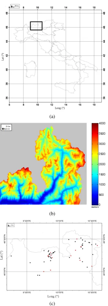
Fig. 1. (a) The study region enclosed in a black rectangle with
lat-itudes (y axes) and longlat-itudes (x axes) expressed. (b) The Digital Elevation Model, related to the study area indicated in (a). The lo-cations of all stations of the initial data set equipped with different types of sensors are marked in figure (c). The locations of the 14 stations equipped with air temperature sensor, snow thickness sen-sor and precipitation gauge, used for the final data set are colored in red.
Fig. 1. (a) The study region enclosed in a black rectangle with
lat-itudes (y-axes) and longlat-itudes (x-axes) expressed. (b) The digital elevation model, related to the study area indicated in (a). The lo-cations of all stations of the initial data set equipped with different types of sensors are marked in figure (c). The locations of the 14 stations equipped with air temperature sensor, snow thickness sen-sor and precipitation gauge, used for the final data set are colored in red.
4 Problem description
Several models and approaches were used to estimate the one-dimensional (z-direction) evolution of snow cover (e.g., Jordan, 1991; Melloh, 1999; Thorsen et al., 2010). When these models use only precipitation and air temperature as input data they require the definition of different physical thresholds. The literature shows that there is no universally accepted method for the evaluation of snow height that can be applied in every condition; often the choice of the most suitable method for the estimation of snow cover thickness (but also of other climatic data) depends on temporal resolu-tion, spatial resoluresolu-tion, data quantity and also on the region of interest. Proceeding from these considerations we propose a model based on the following input variables:
1. Climatic:
(a) Daily min temperature (b) Daily mean temperature (c) Daily max temperature (d) Daily precipitation
(e) Cumulative rain over a given temporal intervalT
(f) Mean of measures in 1a (Daily min temperature) within intervalT
(g) Mean of measures in 1b (Daily mean temperature) within intervalT
(h) Mean of measures in 1c (Daily max temperature) within intervalT.
2. Geographic: (a) Elevation (b) Aspect (c) Slope.
We assume that the value forT, the time interval in which the variables 1a–c are averaged for finding the variable h– f, can be heuristically assessed by a trial and error proce-dure during experiments (see Sect. 7). Based on the above listed climatic and geographic factors, we approach the snow cover thickness estimation as both a function regression and classification problem. In the first case, the output variable
snow cover thickness assumes continuous values; in the
E. Binaghi et al.: Snow cover thickness estimation 845
– Class A: absence of snow cover
– Class B: 1–10 cm
– Class C: 11–90 cm
– Class D: greater than 90 cm.
Table 1 summarizes inputs and outputs for regression and classification tasks.
5 Data set
The data set used was provided by Regione Lombardia1and consists of the climatic series recorded between 1987 and 2003 by 136 climatic sensors located in 64 different loca-tions (Fig. 1c). Unfortunately the series has different tempo-ral length and in many cases large gaps. Moreover the sta-tions were equipped in different ways with different sensors. Consequently the derived data set was built using the spa-tial intersection of stations equipped with the instruments needed; this operation reduced the number of the stations to 16. In order to have comparable data, we decided to use as source of input data only the observations for a restricted time period (2002–2003). With the temporal intersection we obtained the final data set composed of 5476 observations heterogeneously distributed in 14 different locations (Fig. 1c in red). Table 2 lists the final data available for each station distinguished by months. Looking into the details, we ob-serve that May, July and August are the most critical months in which 46 % of the data have gaps. Data related to input variables 1a, 1b, 1c listed in Sect. 4 are instrumental measure-ments drawn directly from the climatic database. Values of variables listed as 1e, 1f, 1g, 1h are obtained by applying cu-mulative and average procedures. Values of geographic vari-ables are extracted from the digital elevation model (DEM) downloaded free of charge from the geoportal of Regione Lombardia and has a spatial resolution of 20 m. Aspect and slope were computed using the dedicated tools (Spatial Ana-lyst Tools) of the ArcGIS 10 (ArcEditor).
6 Radial basis function networks
Our study modeled snow cover thickness estimation as a neu-ral learning task according to which the correlation between climatic/geographic factors and snow cover thickness is in-ferred by induction from supervised input-output pairs of data. We adopt radial basis function networks in both regres-sion and classification task.
1Many geospatial data (vector and raster) are available on the
geoportal related to the Lombardy region http://www.cartografia. regione.lombardia.it/geoportale.
12 :
x1
x2
x3
xk
xk−2
xk−1
hMx
hM−1x h2x h1x
∑ w1
w2
wM−1
wM
fx
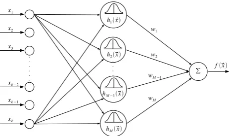
Fig. 2.Radial Basis Function Network architecture for function approximation.
Fig. 2. Radial basis function network architecture for function
ap-proximation.
6.1 RBFN architecture and training algorithm
RBFNs are characterized by a very simple three layer archi-tecture. The input layer propagates input values to a single hidden layer. In the output layer, each neuron receives a lin-ear combination of the output of hidden neurons. In the case of one output node, the global nonlinear function computed by the network can be expressed as a linear combination of
Mbasis functions associated with each hidden layer neuron. In the formula we have
f (x)=
M X
i
wjhj(x), (1)
wherex= [x1, .., xk]T is the K-dimensional input vector,wj are the weighting coefficients of the linear combination and
hj(x) represents the output of the Gaussian shaped basis function, with scale factorrj, associated with thej-th neuron in the second layer. The response ofj-th neuron decreases monotonically with the distance between the input vectorx and the center of each functioncj= [c1j, . . . , ckj]:
hj(x)=exp −
||x−c||2 rj
!
. (2)
During the training phase, the RBFN learns an approxi-mation for the true input–output relationship based on a given training set of examples constituted byNinput-output pairs{xi, yi}, i=1,2, . . . , N. Following Moody and Darken (1989), the training scheme is two-phased:
1. phase one is unsupervised and decides values for cj, j=1, . . . , M,
2. phase two solves a linear problem to find values for
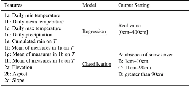
Table 1. Input and output variables used in regression and classification tasks.
Features Model Output Setting 1a: Daily min temperature
Regression
Real value [0cm–400cm] 1b: Daily mean temperature
1c: Daily max temperature 1d: Daily precipitation 1e: Cumulated rain onT 1f: Mean of measures in 1a onT
Classification
A: absence of snow cover B: 1cm–10cm
C: 11cm–90cm D: greater than 90cm 1g: Mean of measures in 1b onT
1h: Mean of measures in 1c onT 2a: Elevation
2b: Aspect 2c: Slope
Table 2. Amount of data in the final dataset. The division into months and altitude has been applied to emphasize the diversity and
incom-pleteness of the data structure.
Months
Station m a.s.l. Jan Feb Mar Apr May Jun Jul Aug Sep Oct Nov Dec Tot Branzi 830 23 25 28 0 0 56 0 0 60 0 0 9 201 Grosio 1220 54 53 31 0 0 55 0 0 60 0 60 42 355 Val Torreggio 1350 17 28 35 30 0 60 0 0 60 31 30 50 341 Val Dorena 1575 46 22 7 0 0 0 0 0 0 4 29 31 139 Laghi di Chiesa 1596 59 56 62 60 2 59 0 0 60 62 59 61 540 Alpe Costa 1672 62 56 62 60 21 59 0 0 60 62 60 62 564 Piazzo Cavalli 1719 62 56 62 60 18 59 0 0 60 62 60 62 561 Monte Masuccio 1770 17 28 31 30 0 30 0 0 30 29 30 31 256 Carona 1955 31 27 30 30 1 30 0 0 30 40 60 52 331 Funivia Bernina 2014 62 56 62 59 32 0 62 62 7 62 60 62 586 Saviore dell’Adamello 2017 0 0 0 0 0 0 31 31 1 28 30 0 121 Cam Boer 2114 62 56 62 52 24 0 46 38 20 55 55 62 532 Monte Trela 2150 55 56 62 60 0 0 59 50 0 62 60 57 521 Isola Persa 2700 31 28 31 30 31 30 31 31 30 33 60 62 428 Tot 581 547 565 471 129 438 229 212 478 530 653 643 5476
The configuration of the model requires two user parame-ters:
1. the numberMof first level local processing units and 2. the number p of the p-means heuristic (Moody and
Darken, 1989), used to determine the scale factor rj,
j=1, . . . , M of basis functions associated with first level processing units.
The second phase, having model parameters M, cj, j=1, . . . , M, rj, j=1, . . . , M known, computes
wi, i=1, . . . , M minimising the difference between pre-dicted output and truth by least mean squares, computed through the pseudo inverse. In formula
w=(HTH)−1HTy=H+y, (3)
where
H=
h1(x1) h2(x1) · · · hM(x1) h1(x2) h2(x2) · · · hM(x2)
..
. ... . .. ... h1(xN) h2(xN)· · ·hM(xN)
(4)
and y= [y1, ..yN] is the vector of output data, w=
[w1, ..wM]T are second level weights. The trained network is tested using a proper set of examples never seen during training.
6.2 Computation: regression and classification
E. Binaghi et al.: Snow cover thickness estimation 847
multidimensional function estimation modeled in the two different settings: regression and classification.
In the regression configuration, the RBFN learns from input-output pairs constituted as usual, by input patterns resented by a vector of measurements and output values rep-resenting numerical function values. The network is config-ured with a single output neuron.
We now formally define the components involved in the regression task. The setis composed of all available data coupled with the relative truth value:
= {(xi, yi), i=1, . . . , N}, (5) wherexi is a vector containing the input variables discussed in Sect. 4,yiis the truth value related toxiandNis the num-ber of available data. The setis then split into two parti-tions, namely the training set TrSand the test set TeS. If the regression task is arbitrary due to the poor reliability of the input data, the multidimensional function estimation can be conveniently modeled as a classification identifying inter-vals of the function codomain and making them correspond with a predefined class. The formal description of the model for classification can be easily obtained from the regression formalization, considering the valueyi in (5) as a label de-scrying membership in each of the defined classes. The net-work is configured with an output layer having a number of neurons equal to the number of classes. During training, in-put pattern vectors are made to correspond with predefined class labels, exemplifying a hard mapping at a lower gran-ularity with respect to regression, with mutually exclusive classes.
7 Experiments
Our experiments adopted different evaluation indexes. The agreement between reference truth and classification results was analyzed by means of the confusion matrix and derived accuracy indexes (Congalton, 1991). A confusion matrix lists the values of the reference data in the columns and the values of the classified data in the rows. The main diagonal of the matrix lists the correctly classified pixels.
– Overall accuracy (OA): OA provides a general
indica-tion of the classifier’s performance. The OA is equal to the ratio between the number of samples correctly classified, summing the values in the main diagonal of the confusion matrix, and the total number of observed samples.
– Producer accuracy (PA): PA measures the
omis-sion(exclusion) errors of the classifier. It is computed for each class. The PA for classit his equal to the ratio between the number of samples correctly classified in classit hand the number of reference samples belong-ing to classit h(columnit htotal).
– User accuracy (UA): UA measures the
commis-sion(inclusion) errors of the classifier. It is computed for each class. The UA for classit his equal to the ra-tio between the number of samples correctly classified in classit hand the total number of samples classified in classit h(rowit htotal).
The performance evaluation obtained using these indexes is complemented by the Cohen’s kappa coefficient believed to be a more robust measure that takes into account the agree-ment occurring by chance (Cohen, 1960).
The kappa formal definition is
K=Pr(a)−Pr(e)
1−Pr(e) , (6)
where Pr(a)=
Pr i=1Xi,i
N (7)
Pr(e)=
Pr
i=1Xi,+X+,i
N2 (8)
and
– r is the number of rows and columns in the confusion matrix;
– Nis the total number of observations;
– Xi,j is the observation in rowiand columnj;
– Xi,+is the marginal total of thei-th row;
– X+,iis the marginal total of thei-th column.
Intuitively, Pr(a) is the proportion of judgments consistent among the classifier and the reference data and Pr(e) is the proportion of agreements that would be observed ran-domly classifying. In contrast to the overall accuracy, Co-hen’s kappa also takes non-diagonal elements into account. To measure the magnitude of network mistakes the root mean square error (RMSE) index and its normalized version NRMSE are used in combination with the mean absolute er-ror (MAE). The formal definition of these index is given be-low:
RMSE=
r 1
n
X
(yˆi−yi)2 (9)
NRMSE= RMSE
MAX(yi)
×100 (10)
MAE= 1 n
X
whereyˆi is the estimated value. The overall data set com-posed of 5476 patterns was randomly split in the propor-tion of 23, 13 for training (TrS) and test (TeS), respec-tively. The radial basis function network configured for the tasks described above was applied to solve the problem of estimating snow cover thickness. The experiments focused on the parameters calibration process. A sensitivity analy-sis was conducted varying the input parameters described in Sect. 6.1. For the training phase focused on centroids identifi-cation, the K-means clustering algorithm was compared with a faster approach based on the random choice ofM points in the input space. These two methods showed comparable performances. However, as the K-means algorithm imposes a small number of centroids to limit the computational com-plexity, the random choice strategy was preferred.
7.1 Regression results
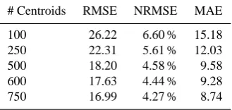
First of all, we present the results obtained using the RBFN configured for the regression task. The RBFN receives in in-put the vector of measurements derived from the set of fea-tures (input variables) described in section 4. Concerning the network architecture, the input layer has 11 neurons equal to the number of features and the output layer has 1 neuron representing the predicted snow height value. Several con-figurations of the RBFN were considered varying the tempo-ral windowT used in the computation of features 1e, 1f, 1g and 1h, which assumed values ranging from 10◦C to 45◦C. For each window size, different RBFN configurations were considered distinguished by the different numberMof basis functions which assumed values 100, 250, 500, 600, 750. The RBFN network showed the best behavior setting the temporal window dimension at 45. Table 3 shows the results obtained in this configuration, varying the neural internal parameter
M. Results are expressed in terms of RMSE, NRMSE and MAE indexes and are obtained training and testing the net-work with five different pairs TrSand TeS, randomly gen-erated from the overall datasetand averaging the individ-ual indexes obtained. Above the value ofM=500 the error indexes significantly decrease for each incremental increase inM. After the valueM=500 the error indexes as a function ofMshow an asymptotic behavior. We than chose than this value as a reference for an optimize balancing between com-putational cost, training accuracy and generalization power. For an in-depth analysis of how the snow cover thickness was modeled, Fig. 3 plots the estimated values versus truth values which are sorted in ascending order. Figure 5a and b show the mean weekly error of the modeled snow cover with re-spect to the weekly mean of the liquid precipitation (rain) of two automatic weather stations (AWS) representative of the lower altitude (ST1) and the higher altitude (ST2) for 2002 and 2003, respectively. There is no significant relationship between the measured liquid precipitation and the errors al-though there is a general increase in errors in late Fall and Spring. At that time the greatest differences of snow height
Table 3. Regression results varying the number of centroidsM,
ex-pressed in terms of RMSE, NRMSE and MAE.
# Centroids RMSE NRMSE MAE 100 26.22 6.60 % 15.18 250 22.31 5.61 % 12.03 500 18.20 4.58 % 9.58 600 17.63 4.44 % 9.28 750 16.99 4.27 % 8.74
at different altitude occur because precipitation is in the form of snow only at higher elevation. Nevertheless, some error peaks (like the first week of 2002 and 2003 and the week 21 of 2003) are clearly not related to the data input. The RMSE values obtained indicate an acceptable mean disagreement between reference and predicted values. However, we have to consider that different intervals within the snow height range have different relevance in the environmental analysis, and errors computed on these intervals become unacceptable making arbitrary numerical predicted values. We proceeded to model snow cover thickness estimation as a classification task.
7.2 Classification results
The criteria with which we introduce classes subdividing snow height intervals, are derived from the idea of using them within a more general study concerning permafrost. The modeling of permafrost is outside the scope of the present paper which is focused on snow depth. Indeed, during the winter, the ground suffers from the extremely low air tem-perature in areas where the snow is absent (class A), while class B (1–10 cm) has been distinguished from C (11–90 cm) because a certain percentage of radiation in class B can reach the ground surface, in addition to the more limited insula-tion of the thinner snow with respect to the air temperature. Above 90 cm (class D) the insulation of the snow can be con-sidered almost total.
E. Binaghi et al.: Snow cover thickness estimation 849
Table 4. Confusion matrix for the radial basis function network
classifier evaluated on the overall test set TeS; Class A: absence of snow cover, Class B: 1–10 cm, Class C: 11–90 cm, Class D: greater than 90 cm.
Reference data
Class A B C D Tot U UA data
A 442 31 5 0 478 92.47 % B 21 377 76 4 478 78.87 % C 2 92 603 15 712 84.69 % D 0 0 17 141 158 89.24 % Tot P 465 500 701 160 – – PA 95.05 % 75.40 % 86.02 % 88.12 % – –
Total accuracy: 85.5969 % (1563 hit, 263 miss, 1826 total) Total error: 14.4031 %
KAPPA value: 79.5523 % KAPPA std.err: 0.0001
Table 5. Confusion matrix for the radial basis function network
classifier evaluated on the test set TeS with elevation below 1000 m; Class A: absence of snow cover, Class B: 1–10 cm, Class C: 11–90 cm, Class D: greater than 90 cm.
Reference data
Class A B C D Tot U UA data
A 38 4 0 0 42 90.48 % B 0 10 3 0 13 76.92 %
C 0 0 0 0 0 //
D 0 0 0 0 0 //
Tot P 38 14 3 0 – – PA 100.00 % 71.43 % 0 % // – – Total accuracy: 87.2727 % (48 hit, 7 miss, 55 total)
Total error: 12.7273 % KAPPA value: 69.1259 % KAPPA std.err: 0.0077
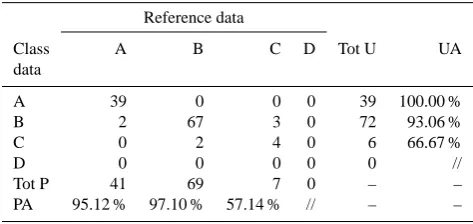
Table 6. Confusion matrix for the radial basis function network
classifier evaluated on the test set TeS with elevation between 1000 and 1300 m; Class A: absence of snow cover, Class B: 1– 10 cm, Class C: 11–90 cm, Class D: greater than 90 cm.
Reference data
Class A B C D Tot U UA
data
A 39 0 0 0 39 100.00 %
B 2 67 3 0 72 93.06 %
C 0 2 4 0 6 66.67 %
D 0 0 0 0 0 //
Tot P 41 69 7 0 – –
PA 95.12 % 97.10 % 57.14 % // – –
Total accuracy: 94.0171 % (110 hit, 7 miss, 117 total) Total error: 5.9829 %
KAPPA value: 88.4322 % KAPPA std.err: 0.0017
Table 7. Confusion matrix for the radial basis function network
classifier evaluated on the test set TeS with elevation between 1300 and 1600 m; Class A: absence of snow cover, Class B: 1– 10 cm, Class C: 11–90 cm, Class D: greater than 90 cm.
Reference data
Class A B C D Tot U UA
data
A 96 7 0 0 103 93.20 %
B 3 96 23 0 122 78.69 %
C 0 17 115 0 132 87.12 %
D 0 0 0 0 0 //
Tot P 99 120 138 0 – –
PA 96.97 % 80.00 % 83.33 % // – –
Total accuracy: 85.9944 % (307 hit, 50 miss, 357 total) Total error: 14.0056 %
KAPPA value: 78.8497 % KAPPA std.err: 0.0008
Table 8. Confusion matrix for the radial basis function network
classifier evaluated on the test set TeS with elevation between 1600 and 1900 m; Class A: absence of snow cover, Class B: 1– 10 cm, Class C: 11–90 cm, Class D: greater than 90 cm.
Reference data
Class A B C D Tot U UA data
A 114 8 1 0 123 92.68 % B 14 95 13 0 122 77.87 % C 0 27 183 0 210 87.14 %
D 0 0 0 0 0 //
Tot P 128 130 197 0 – – PA 89.06 % 73.08 % 92.89 % // – – Total accuracy: 86.1538 % (392 hit, 63 miss, 455 total)
Total error: 13.8462 % KAPPA value: 78.6163 % KAPPA std.err: 0.0006
850 E. Binaghi et al.: Snow cover thickness estimation
Table 9. Confusion matrix for the radial basis function network
classifier evaluated on the test set TeS with elevation between 1900 and 2200 m; Class A: absence of snow cover, Class B: 1– 10 cm, Class C: 11–90 cm, Class D: greater than 90 cm.
Reference data
Class A B C D Tot U UA data
A 155 12 4 0 171 90.64 % B 2 109 34 4 149 73.15 % C 2 46 250 9 307 81.43 % D 0 0 13 53 66 80.30 % Tot P 159 167 301 66 – – PA 97.48 % 65.27 % 83.06 % 80.30 % – –
Total accuracy: 81.8182 % (567 hit, 126 miss, 693 total) Total error: 18.1818 %
KAPPA value: 73.6529 % KAPPA std.err: 0.0004
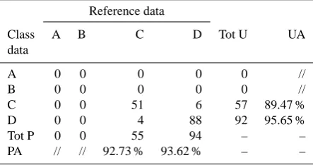
Table 10. Confusion matrix for the radial basis function network
classifier evaluated on the test set TeS with elevation above 2200 m; Class A: absence of snow cover, Class B: 1–10 cm, Class C: 11–90 cm, Class D: greater than 90 cm.
Reference data
Class A B C D Tot U UA data
A 0 0 0 0 0 //
B 0 0 0 0 0 //
C 0 0 51 6 57 89.47 % D 0 0 4 88 92 95.65 % Tot P 0 0 55 94 – – PA // // 92.73 % 93.62 % – – Total accuracy: 93.2886 % (139 hit, 10 miss, 149 total)
Total error: 6.7114 % KAPPA value: 85.6978 % KAPPA std.err: 0.0019
7.3 Snow cover mapping
In order to exploit the potential of RBFN in estimating snow cover distribution, addressed, the production of snow cover maps which offer a synoptic view of the phenomenon un-der investigation. This task was tackled by proceeding in the spatial interpolation of input climatic variables and then by using the RBF network to compute the corresponding pre-dicted snow cover value for each input pattern including cli-mate and geographic input variable. The spatial interpola-tion of temperatures is accomplished considering the varia-tion of this parameter as a funcvaria-tion of the elevavaria-tion (Dodson and Marks, 1997). With reference to a generic cellxy, steps were taken to homogenize the known values in terms of el-evation. Homogenization was obtained by performing linear regression between elevation and temperature values. Setting a reference evaluation value, each known temperature value was shifted as a function of the angular coefficient of the
lin-Fig. 3.Estimated snow cover thickness versus measured values in ascending order.
Fig. 3. Estimated snow cover thickness versus measured values in
ascending order.
ear dependence law. Subsequently spatial interpolation was performed by applying the inverse square distance method obtaining temperature values for each grid unit. These values were finally modified reporting them at the original elevation. The spatial interpolation of precipitation patterns is a critical aspect requiring domain dependent complex analysis. Our study adopted a simple and easily controlled method based on Voronoi tessellation, implicitly assuming that the known values are representative of a given area around the point of measurement (Kay and Kutiel, 1994). We refrained from conducting a more sophisticated analysis that could be arbi-trary in our context. Nine weeks were chosen based on their relevance for permafrost evolution (aggradation/degradation) and their variability. For these reasons, a higher frequency of examined weeks was chosen for the end of the spring (dur-ing the melt(dur-ing period). For each of the nine weeks, a snow map was generated with each grid element representing the neural-computed snow cover thickness.
An indirect validation procedure was accomplished com-paring our results with those obtained by a snow mapping algorithm based on the normalized difference snow index (NDSI) derived from Landsat imagery. The NDSI-based snow algorithm together with its physical assumptions and derived decision rules for producing binary snow cover maps is described in (Dozier, 1989). To proceed in the comparison, neurally computed snow cover thickness values were bina-rized heuristically setting the threshold to a value of 5 cm. This value is a threshold commonly used to define the days with snow on the ground (snow duration) (Hantel and Hirtl-Wielke, 2007). Comparative results have been organized in a confusion matrix in which the classes considered are the presence and absence of snow. Results obtained from NDSI-based snow algorithm serve as of reference data. Table 11 re-ports comparative results in terms of OA (overall accuracy), UA (user accuracy) and PA (producer accuracy) indexes.
E. Binaghi et al.: Snow cover thickness estimation 851
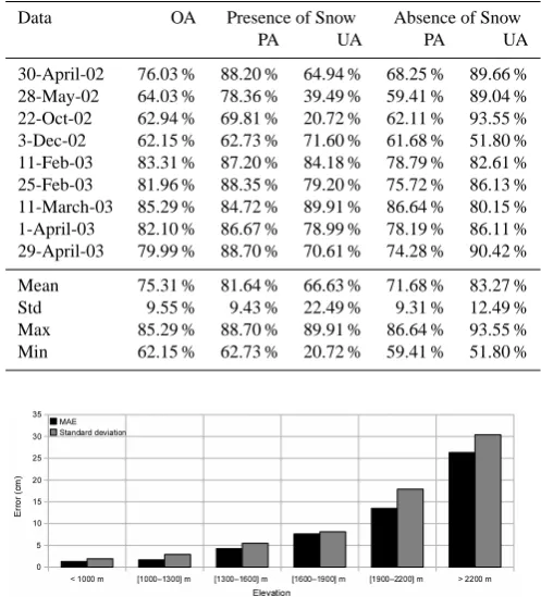
Table 11. Summary of the RBFN results.
Data OA Presence of Snow Absence of Snow
PA UA PA UA
30-April-02 76.03 % 88.20 % 64.94 % 68.25 % 89.66 % 28-May-02 64.03 % 78.36 % 39.49 % 59.41 % 89.04 % 22-Oct-02 62.94 % 69.81 % 20.72 % 62.11 % 93.55 % 3-Dec-02 62.15 % 62.73 % 71.60 % 61.68 % 51.80 % 11-Feb-03 83.31 % 87.20 % 84.18 % 78.79 % 82.61 % 25-Feb-03 81.96 % 88.35 % 79.20 % 75.72 % 86.13 % 11-March-03 85.29 % 84.72 % 89.91 % 86.64 % 80.15 % 1-April-03 82.10 % 86.67 % 78.99 % 78.19 % 86.11 % 29-April-03 79.99 % 88.70 % 70.61 % 74.28 % 90.42 %
Mean 75.31 % 81.64 % 66.63 % 71.68 % 83.27 % Std 9.55 % 9.43 % 22.49 % 9.31 % 12.49 % Max 85.29 % 88.70 % 89.91 % 86.64 % 93.55 % Min 62.15 % 62.73 % 20.72 % 59.41 % 51.80 %
14 :
Fig. 4.Mean Absolute Error and standard deviation in regression task as a function of elevation ranges.
Fig. 4. Mean absolute error (MAE) and standard deviation in
re-gression task as a function of elevation ranges.
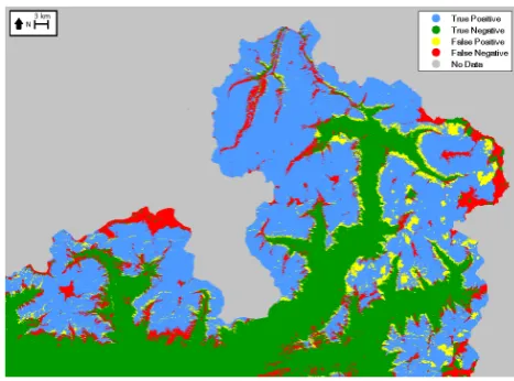
probable on the flat point where AWS are located rather than in the other surrounding areas (generally except for northern exposed slopes). Table 12 shows OA values distinguished by different elevation ranges. Results obtained are gener-ally good at low elevation (<1600 m); at higher elevation, above 1900 m a.s.l., the accuracy decreases below 70 % dur-ing the meltdur-ing season and at the beginndur-ing of Autumn, with a general underestimation. A different result was achieved between 1600 m and 1900 m, where poor results were ob-tained only during the winter core due to a problem of overes-timation. The overall results obtained from the mapping pro-cedure tallied in general with regression and classification re-sults (see Figs. 3 and 4). Figure 6 shows the map produced by the RBF network when processing data for the week 11-03-2003. The overlap of this map, hardened with a 5 cm thresh-old, with the corresponding NDSI map is shown in Fig. 7. A snow scientist examined the maps in light of the topographic features of the study areas, and judged the results satisfac-tory.
7.4 Comparison analysis
A comparison analysis was developed for a quantitative eval-uation of the advantages of the RBFN method with re-spect to conventional widely used spatial interpolation tech-niques when dealing with critical situations originated by
: 15
0 5 10 15 20 25 30 35 40 45 50
0 10 20 30 40 50 60
Time (weeks)
MAE (cm)
0 5 10 15 20 25 30 35 40 45 50
−50
−40
−30
−20
−10 0 10 20 30 40 50
Mean P (cm)
MAE ST1 ST2
(a)
0 5 10 15 20 25 30 35 40 45 50
0 10 20 30 40 50 60
Time (weeks)
MAE (cm)
0 5 10 15 20 25 30 35 40 45 50
−50
−40
−30
−20
−10 0 10 20 30 40 50
Mean P (cm)
MAE ST1 ST2
(b)
Fig. 5.Mean Absolute Error (MAE) in a regression task as a func-tion of weeks during the years 2002 (a) and 2003 (b) compared with the mean weekly liquid precipitation measured close at the altitudi-nal limits of the data set: ST1 485 m a.s.l. and ST2 2150 m a.s.l.
Fig. 5. Mean absolute error (MAE) in a regression task as a function
of weeks during the years 2002 (a) and 2003 (b) compared with the mean weekly liquid precipitation measured close at the altitudinal limits of the data set: ST1 485 m a.s.l. and ST2 2150 m a.s.l.
Table 12. Overall accuracy for 6 elevation ranges.
Date Overall accuracy
0–1000 1000–1300 1300–1600 1600–1900 1900–2200 >2200 30-April-02 99.95 % 94.69 % 99.82 % 82.73 % 56.13 % 68.14 % 28-May-02 99.98 % 98.98 % 99.99 % 91.41 % 47.42 % 42.61 % 22-Oct-02 99.30 % 96.25 % 99.14 % 91.94 % 58.70 % 37.15 % 3-Dec-02 70.60 % 51.78 % 50.82 % 55.14 % 74.42 % 61.33 % 11-Feb-03 99.67 % 91.98 % 93.60 % 67.60 % 60.77 % 87.44 % 25-Feb-03 99.98 % 96.32 % 98.79 % 72.89 % 46.92 % 86.17 % 11-March-03 99.93 % 97.40 % 94.43 % 73.35 % 69.26 % 86.51 % 1-April-03 99.78 % 99.80 % 99.48 % 84.02 % 65.42 % 77.13 % 29-April-03 99.97 % 98.31 % 99.92 % 91.96 % 61.96 % 71.93 % Mean 96.57 % 91.72 % 92.89 % 79.01 % 60.11 % 68.71 % Std 9.74 % 15.16 % 15.96 % 12.73 % 9.18 % 18.66 % Max 99.98 % 99.80 % 99.99 % 91.96 % 74.42 % 87.44 % Min 70.60 % 51.78 % 50.82 % 55.14 % 46.92 % 37.15 %
16 :
Fig. 6.Display on a logarithmic scale of the snow map produced by RBFN.
Fig. 6. Display on a logarithmic scale of the snow map produced by
RBFN.
(29 April 2003). Both the full winter conditions and the early melting are crucial for several environmental issues, but mainly, for permafrost distribution because the snow-free ar-eas in winter (above all at altitudes higher than 2200 m a.s.l. where air temperature are several degrees below 0◦C) are fa-vorable for permafrost aggradation/conservation because the ground can be deeply frozen. On the other hand, the areas where snow melting is late-lying (and therefore later than the end of April, in this area) is also favorable for permafrost formation because positive air temperatures are prevented by the late snow cover.
Consistent with the procedure described in the previous section, maps produced by all the three methods were bi-narized setting the threshold value to 5 cm. Table 13 shows the OA values obtained by RBFN, IDW and Spline, distin-guished by different elevation ranges consistently with the
: 17
Fig. 7.Overlapping of maps produced by the RBFN Network and NDSI. Considering the RBFN map as the first result and the NDSI map as the second, colors have the following meaning: Blue=PS-PS; Green= AS-AS; Yellow= PS-AS; Red=AS-PS, with PS=Presence of Snow and AS=Absence of Snow
Fig. 7. Overlapping of maps produced by the RBFN Network
and NDSI. Considering the RBFN map as the first result and the NDSI map as the second, colors have the following meaning: Blue = PS-PS; Green = AS-AS; Yellow = PS-AS; Red = AS-PS, with PS = Presence of Snow and AS = Absence of Snow
E. Binaghi et al.: Snow cover thickness estimation 853
Table 13. Comparison analysis among IDW, B-Spline and RBF: the results are presented in terms of overall accuracy for 6 elevation ranges.
Overall accuracy Mean Var
Date Methods 0–1000 1000–1300 1300–1600 1600–1900 1900–2200 >2200
11-Feb-03 RBF 99.67 % 91.98 % 93.60 % 67.60 % 60.77 % 87.44 % 83.51 % 15.62 %
DW 7.46 % 12.90 % 15.45 % 29.50 % 59.86 % 85.58 % 35.12 % 31.10 %
Spline 85.44 % 53.35 % 45.38 % 52.01 % 67.17 % 74.20 % 62.92 % 15.30 %
25-Feb-03 RBF 99.98 % 96.32 % 98.79 % 72.89 % 46.92 % 86.17 % 83.51 % 20.63 %
IDW 7.47 % 9.68 % 11.07 % 17.95 % 41.86 % 80.64 % 28.11 % 28.66 %
Spline 84.64 % 50.03 % 42.46 % 44.18 % 53.45 % 70.85 % 57.60 % 16.68 %
29-April-03 RBF 99.97 % 98.31 % 99.92 % 91.96 % 61.96 % 71.93 % 87.34 % 16.38 %
IDW 60.41 % 35.13 % 30.97 % 27.23 % 33.62 % 58.42 % 40.96 % 14.56 %
Spline 49.92 % 46.93 % 40.46 % 38.76 % 39.39 % 53.46 % 44.82 % 6.17 %
8 Conclusions
A method for snow cover thickness estimation is proposed within the context of a Permafrost studies in an alpine envi-ronment, based on the use of a radial basis function network capable of moving from regression and classification tasks which are usually complementary for understanding complex environmental phenomena at different levels of precision. As seen in the experimental context, the learning and approxi-mation capabilities of the network allow the user to overcome the limitations of available data characterized by such criti-cal aspects as the minimal set of climatic and topographic data and the reduced set of non-homogeneously distributed instrumented sites. The comparison analysis conducted be-tween IDW, Spline interpolation techniques and the proposed model demonstrates the superiority of the neural implemen-tation with respect to conventional deterministic approaches. The overall quantitative and qualitative evaluations of the ex-perimental work substantiates the general claim that a va-riety of problems in hydrology and water resources studies benefit from the use of neural techniques, demonstrating in particular the performances of the RBFN model in the spe-cific field of snow cover thickness estimation where its use is still little known. The results of our experiments suggest that RBFN approximation can provide a valuable solution for studies conducted in all mountain areas at high elevations where there are fewer weather stations and where permafrost and glaciers are more prevalent.
Acknowledgements. Work partially supported by the Italian MIUR
project PRIN 2008 “Permafrost e piccoli ghiacciai alpini come elementi chiave della gestione delle risorse idriche in relazione al cambiamento climatico”.
Edited by: J. L. Bamber
References
Agarwal, A., Mishra, S., Ram, S., and Singh, J.: Sim-ulation of Runoff and Sediment Yield using Artifi-cial Neural Networks, Biosyst. Eng., 94, 597–613, doi:10.1016/j.biosystemseng.2006.02.014, 2006.
Antoni, O., Krian, J., Marki, A., and Bukovec, D.: Spatio-temporal interpolation of climatic variables over large region of complex terrain using neural networks, Ecol. Model., 138, 255–263, 2001. Belward, A., Binaghi, E., Lanzarone, G., and Tosi, G. (Eds.): Geospatial Knowledge Processing for Natural Resource Man-agement, vol. 24 of Special Issue of International Journal of Re-mote Sensing, Taylor & Francis, 2003.
Benediktsson, J., Swain, P., and Ersoy, O.: Neural network ap-proaches versus statistical methods in classification of multi-source remote sensing data, IEEE T. Geosci. Remote, 28, 540– 552, 1990.
Binaghi, E., Madella, P., Grazia Montesano, M., and Rampini, A.: Fuzzy contextual classification of multisource remote sensing images, IEEE T. Geosci. Remote, 35, 326–340, doi:10.1109/36.563272, 1997.
Binaghi, E., Brivio, P., Ghezzi, P., Rampini, A., and Zilioli, E.: In-vestigating the Behaviour of Neural and Fuzzy-Statistical Clas-sifiers in Sub-Pixel Land Cover Estimation, Canad. J. Remote Sens., 25, 171–188, 1999.
Binaghi, E., Boschetti, M., Brivio, P., Gallo, I., Pergalani, F., and Rampini, A.: Prediction of displacements in unstable areas using a neural model, Nat. Hazards, 32, 135–154, 2004.
Bishop, C.: Neural networks for pattern recognition, Oxford Uni-versity Press, USA, 1995.
Civco, D.: Artificial neural networks for land-cover classification and mapping, Int. J. Geogr. Inf. Sci., 7, 173–186, 1993. Cohen, J.: A coefficient of agreement for nominal scales, Educ.
Psy-chol. Meas., 20, 37–46, 1960.
Congalton, R.: A review of assessing the accuracy of classifica-tions of remotely sensed data, Remote Sens. Environ., 37, 35–46, 1991.
Coulibaly, P., Bob´ee, B., and Anctil, F.: Improving extreme hy-drologic events forecasting using a new criterion for artifi-cial neural network selection, Hydrol. Process., 15, 1533–1536, doi:10.1002/hyp.445, 2001.
Crane, R. G. and Anderson, M. R.: Satellite discrimination of snow/cloud surfaces, Int. J. Remote Sens., 5, 213–223, doi:10.1080/01431168408948799, 1984.
Dell’Acqua, F. and Gamba, P.: Pyramidal rain field decomposition using radial basis function neural networks for tracking and fore-casting purposes, IEEE T.Geosci. Remote, 41, 853–862, 2003. Dobreva, I. D. and Klein, A. G.: Fractional snow cover
map-ping through artificial neural network analysis of {MODIS} surface reflectance, Remote Sens. Environ., 115, 3355–3366, doi:10.1016/j.rse.2011.07.018, 2011.
Dodson, R. and Marks, D.: Daily air temperature interpolated at high spatial resolution over a large mountainous region, Climate Res., 8, 1–20, doi:10.3354/cr008001, 1997.
Dozier, J.: Spectral signature of alpine snow cover from the Land-sat Thematic Mapper, Remote Sens. Environ., 28, 9–22, http: //linkinghub.elsevier.com/retrieve/pii/0034425789901016, 1989. Foody, G.: Land cover classification by an artificial neural network with ancillary information, Int. J. Geogr. Inf. Sci., 9, 527–542, 1995.
Gardner, M. and Dorling, S.: Artificial neural networks (the multi-layer perceptron) – A review of applications in the atmospheric sciences, Atmos. Environ., 32, 2627–2636, 1998.
Gong, P.: Integrated analysis of spatial data from multiple sources: using evidential reasoning and artificial neural network tech-niques for geological mapping, Photogramm. Eng. Remote Sens., 62, 513–523, 1996a.
Gong, P.: Integrated analysis of spatial data from multiple sources: using evidential reasoning and artificial neural network tech-niques for geological mapping, Photogramm. Eng. Remote Sens., 62, 513–523, 1996b.
Gray, D. and Male, D.: Handbook of Snow: Principles, Processes, Management & Use, Blackburn Press, http://books.google.it/ books?id=zhZFPgAACAAJ, 2004.
Guidali, A., Binaghi, E., Guglielmin, M., and Pascale, M.: Investi-gating the Behaviour of Radial Basis Function Networks in Re-gression and Classification of Geospatial Data, in: IDEAL’10, 110–117, 2010.
Guzzetti, F., Carrara, A., Cardinali, M., and Reichenbach, P.: Land-slide hazard evaluation: a review of current techniques and their application in a multi-scale study, Central Italy, Geomorphology, 31, 181–216, 1999.
Hantel, M. and Hirtl-Wielke, L.-M.: Sensitivity of Alpine snow cover to European temperature, Int. J. Climatol., 27, 1265–1275, doi:10.1002/joc.1472, 2007.
Hush, D. and Horne, B.: Progress in supervised neural networks, IEEE Signal Proc. Mag., 10, 8–39, 1993.
Jain, A., Mao, J., and Mohiuddin, K.: Artificial neural networks: A tutorial, Computer, 29, 31–44, 1996.
Jayawardena, A., Fernando, D., and Zhou, M.: Comparison of mul-tilayer perceptron and radial basis function networks as tools for flood forecasting, IAHS-AISH P., 239, 173–182, 1997.
Jordan, R.: A one-dimensional temperature model for a snow cover: Technical documentation for SNTHERM. 89., CRREL Special Report 91-16, US Army Cold Regions Research and Engineering Laboratory, Hanover, NH, 1991.
Kay, P. A. and Kutiel, H.: Some remarks on climate maps of precip-itation, Climate Res., 4, 233–241, 1994.
Lee, S., Ryu, J., Min, K., and Won, J.: Landslide susceptibility anal-ysis using GIS and artificial neural network, Earth Surf. Proc. Land., 28, 1361–1376, 2003.
Lees, B. G.: Neural network applications in the geosciences: An in-troduction, Comput. Geosci., 22, 955–957, doi:10.1016/S0098-3004(96)00033-7, 1996.
Leuangthong, O., McLennan, J., and Deutsch, C.: Minimum Accep-tance Criteria for Geostatistical Realizations, Nat. Resour. Res., 13, 131–141, doi:10.1023/B:NARR.0000046916.91703.bb, 2004.
Melloh, R.: A synopsis and comparison of selected snowmelt algo-rithms, CRREL Report 99-8, US Army Cold Regions Research and Engineering Laboratory. Hanover, NH, 1999.
Moody, J. and Darken, C.: Fast learning in networks of locally-tuned processing units, Neural Comput., 1, 281–294, 1989. Moradkhani, H., Hsu, K., Gupta, H., and Sorooshian, S.: Improved
streamflow forecasting using self-organizing radial basis func-tion artificial neural networks, J. Hydrol., 295, 246–262, 2004. Park, J. and Sandberg, I. W.: Universal approximation using
radial-basis-function networks, Neural Comput., 3, 246–257, doi:10.1162/neco.1991.3.2.246,, 1991.
Philip, N. S. and Joseph, K. B.: A neural network tool for analyzing trends in rainfall, Comput. Geosci., 29, 215–223, 2003. Sauter, T., Weitzenkamp, B., and Schneider, C.: Spatio-temporal
prediction of snow cover in the Black Forest mountain range us-ing remote sensus-ing and a recurrent neural network, Int. J. Clima-tol., 30, 2330–2341, doi:10.1002/joc.2043, 2010.
Simpson, J. and McIntire, T.: A recurrent neural network classifier for improved retrievals of areal extent of snow cover, IEEE T. Geosci. Remote, 39, 2135–2147, doi:10.1109/36.957276, 2001. Sun, C., Neale, C., McDonnell, J., and Cheng, H.-D.: Monitoring
land-surface snow conditions from SSM/I data using an artificial neural network classifier, IEEE T. Geosci. Remote, 35, 801–809, doi:10.1109/36.602522, 1997.
Tabios, G. Q. and Salas, J. D.: A comparative analysis of techniques for spatial interpolation of precipitation1, J. Am. Water Resour. As., 21, 365–380, doi:10.1111/j.1752-1688.1985.tb00147.x, 1985.
Tagliaferri, R., Longo, G., D’Argenio, B., and Incoronato, A.: In-troduction: Neural networks for analysis of complex scientific data: astronomy and geosciences, Neural Networks, 16, 295– 295, doi:10.1016/S0893-6080(03)00012-1, 2003.
Tedesco, M., Pulliainen, J., Takala, M., Hallikainen, M., and Pam-paloni, P.: Artificial neural network-based techniques for the re-trieval of{SWE}and snow depth from SSM/I data, Remote Sens. Environ., 90, 76–85, doi:10.1016/j.rse.2003.12.002, 2004. Thorsen, S., Roer, A., and Van Oijen, M.: Modelling the dynamics
of snow cover, soil frost and surface ice in Norwegian grasslands, Polar Res., 29, 110–126, 2010.