A model of gene-gene and gene-environment interactions and its implications for targeting environmental interventions by genotype

Open Access

Research

A model of gene-gene and gene-environment interactions and its

implications for targeting environmental interventions by genotype

Helen M Wallace*

Address: GeneWatch UK, The Mill House, Tideswell, Buxton, Derbyshire, SK17 8LN, UK Email: Helen M Wallace* - [email protected]

* Corresponding author

Abstract

Background: The potential public health benefits of targeting environmental interventions by genotype depend on the environmental and genetic contributions to the variance of common diseases, and the magnitude of any gene-environment interaction. In the absence of prior knowledge of all risk factors, twin, family and environmental data may help to define the potential limits of these benefits in a given population. However, a general methodology to analyze twin data is required because of the potential importance of gene interactions (epistasis), gene-environment interactions, and conditions that break the 'equal gene-environments' assumption for monozygotic and dizygotic twins.

Method: A new model for gene-gene and gene-environment interactions is developed that abandons the assumptions of the classical twin study, including Fisher's (1918) assumption that genes act as risk factors for common traits in a manner necessarily dominated by an additive polygenic term. Provided there are no confounders, the model can be used to implement a top-down approach to quantifying the potential utility of genetic prediction and prevention, using twin, family and environmental data. The results describe a solution space for each disease or trait, which may or may not include the classical twin study result. Each point in the solution space corresponds to a different model of genotypic risk and gene-environment interaction.

Conclusion: The results show that the potential for reducing the incidence of common diseases using environmental interventions targeted by genotype may be limited, except in special cases. The model also confirms that the importance of an individual's genotype in determining their risk of complex diseases tends to be exaggerated by the classical twin studies method, owing to the 'equal environments' assumption and the assumption of no gene-environment interaction. In addition, if phenotypes are genetically robust, because of epistasis, a largely environmental explanation for shared sibling risk is plausible, even if the classical heritability is high. The results therefore highlight the possibility – previously rejected on the basis of twin study results – that inherited genetic variants are important in determining risk only for the relatively rare familial forms of diseases such as breast cancer. If so, genetic models of familial aggregation may be incorrect and the hunt for additional susceptibility genes could be largely fruitless.

Published: 09 October 2006

Theoretical Biology and Medical Modelling 2006, 3:35 doi:10.1186/1742-4682-3-35

Received: 13 April 2006 Accepted: 09 October 2006 This article is available from: http://www.tbiomed.com/content/3/1/35

© 2006 Wallace; licensee BioMed Central Ltd.

Background

Some geneticists have predicted a genetic revolution in healthcare: involving a future in which individuals take a battery of genetic tests, at birth or later in life, to determine their individual 'genetic susceptibility' to disease [1,2]. In theory, once the risk of particular combinations of geno-type and environmental exposure is known, medical interventions (including lifestyle advice, screening or medication) could then be targeted at high-risk groups or individuals, with the aim of preventing disease [3].

However, there are also many critics of this strategy, who argue that it is likely to be of limited benefit to health [4-8]. One area of debate concerns the proportion of cases of a given common disease that might be avoided by target-ing environmental or lifestyle interventions to those at high genotypic risk. Known genetic risk factors have to date shown limited utility in this respect [9]. However, some argue that combinations of multiple genetic risk fac-tors may prove more useful in the future [10].

There are two possible approaches to considering this issue. The 'bottom-up' approach seeks to identify individ-ual genetic and environmental risk factors and their inter-actions and quantify the risks. However, this approach is limited by the difficulties in establishing the statistical validity of genetic association studies and of quantifying gene-gene and gene-environment interactions: see, for example, [11-14].

A 'top-down' approach instead considers risks at the pop-ulation level using twin and family studies and data on the importance of environmental factors in determining a trait. However, analysis of twin data is usually limited by the assumptions made in the classical twin study [15], including that: (i) there are no gene-gene interactions (epistasis); (ii) there are no gene-environment interac-tions; (iii) the effects of environmental factors shared by twins are independent of zygosity (the 'equal environ-ments' assumption). These assumptions have all been individually explored and shown to be important in influ-encing the conclusions drawn from twin and family data [16-18]. In addition, the magnitude of any gene-environ-ment interaction is critically important in determining the utility of targeting environmental interventions by geno-type [19]. Although a general methodology to analyze twin data without making these assumptions has been developed, the algebra becomes intractable once multiple loci are involved [17]. This is problematic because, for common diseases, the impacts of multiple genetic vari-ants, and potentially the whole genetic sequence, on dis-ease susceptibility (here called 'genotypic risk') may be important.

The four-category model of population risks developed by Khoury and others [19] is a useful starting point for a top-down analysis of genetic prediction and prevention. It allows the merits of a targeted intervention strategy (which seeks to reduce the exposure of the high-risk gen-otype group only) to be explored, and can readily be extended to include more than four risk categories [10]. However, this model's use to date has been limited to bot-tom-up consideration of single genetic variants or to stud-ying hypothetical examples of multiple variants. The four-category model is limited by the assumption of no con-founders, which means it is applicable to only a subset of possible models of gene-gene and gene-environment interaction. However, situations where the 'no confound-ers' assumption is valid are arguably most likely to be of relevance to public health.

The aim of this paper is to combine the four-category model with population level data from twin, family and environmental studies, without adopting the classical twin model assumptions. This model of gene-gene and gene-environment interactions is then used to implement a 'top-down' approach to quantifying the utility of genetic 'prediction and prevention'.

Method

The four-category model

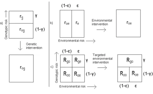
Consider a population divided into genotypic or environ-mental risk categories for a given trait (Figure 1a and 1b). The fraction of the population in the 'high environmental risk group' (designated by subscript e) is ε, and this sub-population is at risk r_e. The remainder of the population is at risk r_oe. The fraction of the population in the 'high genotypic risk' group (designated by the subscript g) is γ, and this subpopulation is at risk r_g, with the remainder of the population at risk r_og. The total risk r_t for this trait in this population is then given by:

rt = γrg + (1-γ)rog (1)

or by:

r_t = εr_e + (1-ε)r_oe (2)

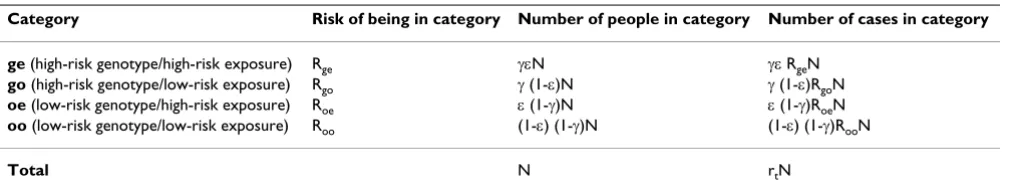
The same population can alternatively be divided into four categories, making a four-category model (Figure 1c)) with risks Roo, Roe, Rgo and Rge. Table 1 shows the risk categories in this model.

The risks are related to the previous definitions by:

r_g = εR_ge + (1-ε) R_go (3)

r_e = γR_ge + (1-γ) R_oe (5)

r_oe = γR_og + (1-γ) R_oo (6)

The category risks R remain constant in different popula-tions (i.e. as ε and γ vary), provided there are no con-founders. This assumption restricts the model to special cases of gene-gene and gene-environment interaction. Note that for a single genetic variant, r_g corresponds to the penetrance of the variant, and that in general (provided R_ge ≠ R_go) this varies with the proportion of the population in the high exposure group, ε, as has been observed [20,21].

The total risk for the given trait is given by:

r_t = γεR_ge + γ(1-ε)R_go + ε(1-γ)R_oe + (1-ε)(1-γ)R_oo (7)

The subpopulation of cases has different characteristics from the general population: for example, it contains a higher proportion of people from the 'ge' subgroup. The relative risk for a person drawn randomly from a subpop-ulation with the same genotypic and environmental

char-acteristics as the cases, RRcases_{, is given by the sum of the} relative risks for each category shown in Table 1:

Similarly, the relative risk for a person drawn randomly from a subpopulation with the same genotypic character-istics as the cases (but with the environmental characteris-tics of the general population) is:

The relative risk for a person drawn randomly from a sub-population with the same environmental characteristics as the cases (but with the genotypic characteristics of the general population) is:

RR R R R R

r

cases ge go oe oo

t

= γε +γ −ε +ε −γ + −ε −γ ( )

2 2 2 2

2

1 1 1 1

8

( ) ( ) ( )( )

RR r r

r

gen

cases g og

t

=γ + −γ

( )

2 2

2

1

9

( )

RR r r

r

env

cases e oe

t

=ε 2+ −(1₂ ε) 2

( )

10

The four-category model

Figure 1

Population attributable fractions

Provided there are no confounders, the population attrib-utable fraction (PAFE

e) due to the presence of the high exposure (E) in the high exposure population subgroup (e) may be defined as:

If the trait is a disease, PAFE

e is the proportion of cases that could be avoided if an environmental intervention (such as a lifestyle change or reduction in exposure) succeeds in moving everyone in the 'high environmental risk group' to the 'low environmental risk' category, as shown in Fig-ure 1b.

The targeted population attributable fraction (PAFE ge) may be defined as the proportion of cases that could be avoided by targeting the same environmental interven-tion at the 'high genotypic + high environmental risk' sub-group only (the 'ge' subsub-group), as shown in Figure 1c. Again assuming no confounders, it is given by:

Note that PAFE

ge differs from PAFge as defined by Khoury & Wagener [19]. The latter implicitly assumes that both environmental and genetic risk factors are reduced and thus is inappropriate for assessing the merits of a targeted environmental intervention. PAFE

ge as defined here is instead equivalent to the targeted attributable fraction (AFT) defined by Khoury et al. [10]. To avoid confusion, the notation adopted here specifies both the nature of the intervention (environmental, denoted by superscript E) and the target subpopulation (the 'ge' subgroup, at both high genotypic and high environmental risk). Thus, the proportion of cases that would be avoided were it possible to move the 'high genotypic risk' subgroup to 'low geno-typic risk' (as shown in Figure 1a) is written as PAFG

g, given by:

Although in practice it is not possible to change the geno-type of the population, the parameter PAFG

g is neverthe-less useful in the calculations that follow.

Measures of utility

Khoury et al. [10] define the Population Impact (PI) as:

PI is one possible measure of the usefulness of targeting the environmental intervention (E) at the 'ge' subgroup. It measures the proportion of cases avoided by targeting the 'high genotypic + high environmental risk' subgroup (the 'ge' subgroup), compared to the proportion avoided by applying the environmental intervention to the whole 'high environmental risk' group. PI has the property:

0 ≤PI ≤ 1 (15)

and has its maximum value when PAFE

ge = PAFEe. How-ever, as a measure of the utility of genotyping, PI has the disadvantage that it takes no account of the proportion of the population γ in the high genotypic risk group. This means PI = 1 when γ = 1 simply because the whole popu-lation is then in the high genotypic risk group, although using genotyping to target environmental interventions is more likely to be useful if PI = 1 and γ is also small.

Therefore, consider an alternative utility parameter U_ge, defined by:

which has the property

-γ≤U_ge ≤ (1-γ) (17)

Uge tends to 1 only if PI = 1 and γ is also small. It is a meas-ure of the utility of using genotyping to target the environ-mental intervention at the 'ge' subgroup, compared to randomly selecting the same proportion γ of the popula-tion to receive the intervenpopula-tion. U_ge is positive if those at high genotypic risk have more to gain than those at low PAF r r

r R R R R r

eE e oe

t ge go oe oo t

=ε( − )=ε γ

{

( − ) (+ −1 γ)( − )

}

( )11

PAF_geE =εγ(R_ge−R_go)/r_t

( )

12

PAF r r

r R R R R r

gG

g og

t ge oe go oo t

=γ( − )=γ ε

{

( − ) (+ −1 ε)( − )

}

( )13

PI=PAFgeE PAFeE

( )

14

U PAF PAF

R R R R

R R

ge geE eE

ge go oe oo

ge go

= − = −  − − − 

− +

γ γ γ

γ

( ) ( ) ( )

( )

1

((1− )( − ) 16

 γ R_oe R_oo  ( )

Table 1: The four category model: risks and cases for a population of size N.

Category Risk of being in category Number of people in category Number of cases in category

ge (high-risk genotype/high-risk exposure) Rge γεN γε RgeN

go (high-risk genotype/low-risk exposure) R_go γ (1-ε)N γ (1-ε)R_goN

oe (low-risk genotype/high-risk exposure) R_oe ε (1-γ)N ε (1-γ)R_oeN

oo (low-risk genotype/low-risk exposure) R_oo (1-ε) (1-γ)N (1-ε) (1-γ)R_ooN

genotypic risk from the intervention ((R_ge-R_go) ≥ (R_oe -R_oo)) and negative if they have less to gain from the inter-vention. This reflects the fact that targeting those who have least to gain through an intervention is worse than using random selection in terms of its impact on popula-tion health.

Note that even if genotyping is better than random selec-tion, other types of test that are more useful may be avail-able [22]; a population-based approach still has the potential to reduce more cases of disease [9,19,23]; and such targeting also has broader psychological and social implications. Therefore a positive U_ge does not necessarily imply that genotyping is the best means of selecting a sub-population to target, or that a targeted approach is neces-sarily effective or socially acceptable. Note also that the measure U_ge applies only to interventions that are consid-ered applicable to the whole population (such as smoking cessation) and neglects other relevant issues such as cost-effectiveness and the burden of disease [24]. In addition, it is necessary to consider the magnitude of the Popula-tion Attributable FracPopula-tion, PAFE

e before proposing this approach. This is because both PI and Uge may tend to unity even if only a small proportion of cases can be avoided by means of environmental interventions.

Limits on parameters

Consider only populations where r_g ≥ r_og and r_e ≥ r_oe for all values of ε and γ. Then the risks in the four box model must be ordered such that:

1 ≥R_ge ≥R_oe ≥R_oo ≥ 0 (18)

and

R_ge ≥R_go ≥R_oo (19)

Using the known relationships (Equations (11), (13) and (16)) between PAFE

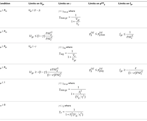
e, PAFGg, Uge and the risks Roo, Rgo, Roe and R_ge, leads to the limits on the utility parameter U_ge shown in Table 2. These conditions also ensure that PAFE

e, PAFG

g and PAFEge are all positive. The two remaining ine-qualities (R_ge ≤ 1 and R_oo ≥ 0) are considered later, where they are used to derive limits on the proportion of the population in the 'high genotypic risk' group, γ. This step is not possible at this stage because PAFE

e, PAFGg and PAFE

ge are themselves dependent on γ. The twin and familial risks model

Data from studies of monozygotic and dizygotic twins are commonly used to estimate the genetic and environmen-tal variances V_g and V_e of a trait. Here, the aim is to use twin and other data to estimate the possible magnitudes of the population attributable fractions and measures of utility defined above. To do this it is necessary to estimate

V_g, V_e and the variance due to gene-environment interac-tion, V_ge. The standard methodology for twin data analysis is inappropriate because it assumes V_ge = 0.

First note that we are interested in the extent to which rel-atives share risk categories (which may be either environ-mental or genotypic, or both), rather than a particular genetic variant. The probability that a relative of a proband is also a case depends on the extent to which their environmental and genotypic risks are correlated with those of the proband. Rather than adopting a specific form for the genetic model, define prel

g as the correlation in genotypic risk category (g) between relatives of type denoted by the superscript 'rel'. The parameter prel

g is the probability that the genotypic risk category (high or low) is identical by descent.

For monozygotic (MZ) twins, assumed to share their entire genome, pMZ

g = 1. For dizygotic (DZ) twins and other siblings, who share half their genome, pDZ

g = psibg = 1/2 for a single allele model (dominant Mendelian disor-der) or an additive polygenic model. For a two allele model (recessive Mendelian disorder) or the dominance term of a polygenic model (in which multiple pairs of alleles interact), pDZ

g = psibg = 1/4. Here, allowing for the possibility of multiple gene-gene interactions (epistasis), require only that:

The meaning of pDZ

g and its relationship to the polygenic risk model first adopted by Ronald Fisher in 1918 is dis-cussed further below.

Similarly, define prel

e as the correlation in environmental risk category (e) between relatives of type "rel", requiring only that:

Assume that prel

g and prele are independent (so that there is no genotype-environment correlation) and that risks within a category are randomly distributed. The relative risk for a relative of type "rel" may then be written:

Substituting for the relative risks RRcases

gen, RRcasesenv and RRcases _{using Equations (8), (9) and (10) leads (after some} algebra) to:

where

1 2≥p_gDZ ≥0

( )

20

1≥p_erel ≥0

( )

21

λrel= −(1 pgrel)(1−perel)+prelg(1−prele)RRcasesgen + −(1 prelg)pp RRerel envcases+p p RRgrelerel cases ( )22

λrel grel g

t

erel e t

g rel

erel ge

t

p V

r

p V

r

p p V

r

− =1 + +

( )

23

Note that if the G-E interaction component of the vari-ance, V_ge, is zero, the utility of targeting the environmental intervention by genotype, Uge, is also zero (Equation (26)), because those at high genotypic risk have no more to gain from the intervention than those at low genotypic risk (R_ge-R_go = R_oe-R_oo).

Equation (23) can also be derived more formally using matrix methods (Appendix A).

The gene-environment interaction factor and remaining inequalities

Without loss of generality, define the gene-environment interaction factor f_ge such that:

and choose its sign so that (combining Equations (24), (25) and (26)):

U_ge is zero if f_ge = 0 (i.e. for an additive G-E model, with no G-E interaction), but for a given γ and V_g, U_ge increases with increasing gene-environment interaction factor, f_ge. For a fixed f_ge and genetic variance component V_g, U_ge is maximum when γ = 1/2, i.e. when half the population is in the high genotypic risk group, provided solutions with

γ = 1/2 exist (see also below: cases where γ_maxge < 1/2). Using the definitions of V_e, V_g and V_ge (Equations (24), (25) and (26)) and the remaining inequalities, R_ge ≤ 1 and R_oo ≥ 0, two limits can be derived on the proportion of the population in the 'high genotypic risk' group, γ (see Table 2).

Scoping studies

The general system of equations represented by Equation (23) may be simplified where data exist from monozy-gotic twins, dizymonozy-gotic twins and other siblings, such that

λ_DZ > λ_sib. This implies that environmental risks are more strongly correlated in dizygotic twins than in other sib-lings, pe

DZ > pesib. Remembering that pMZg = 1 and psibg = pDZ

g, three independent equations for the relative risk in monozygotic, dizygotic twins and siblings may then be written:

To solve, assume the recurrence risks λ are known (see Appendix B and [25]) and define:

with

R_MD ≥ 1 (34)

and

0 ≤R_SD ≤ 1. (35)

Note that if R_SD = 1, Equations (30) and (31) are identical, pe

DZ = pesib, and more relatives are needed to obtain solu-tions, except in the special case where there is no environ-mental variance (see below: no environmental variance).

In addition, define the variable parameters (assumed unknown):

with

c_MD ≥ 1 (38)

V r PAF e t eE 2 2 1 24 = −  

( )

( ε) ε V r PAF g t gG 2 2 1 25 = −( γ)_ _

( )

γ V r U PAF ge t

ge eE

2 2 1 1 26 = − −  

( )

( ) ( ) ε εγ γ V r f V r V r ge t ge g t e t 2 2

2 2 27

= .

( )

U f V

r

ge ge

g

t

= γ(1−γ) ₂

( )

28

λMZ

g

t

eMZ e t e MZ ge t V r p V r p V r

− =1 + +

( )

29

2 2 2

λDZ gDZ

g

t

eDZ e t g DZ eDZ ge t p V r p V r

p p V

r

− =1 + +

( )

30

2 2 2

λsib gDZ g

t

esib e t g DZ esib ge t p V r p V

r p p

V

r

− =1 ₂ + ₂ + ₂

( )

31

RMD MZ

DZ = − −

( )

λ λ 1 1 32

R_SD sib

DZ = − −

( )

λ λ 1 1 33 c p p MD e MZ eDZ

=

( )

36

c p

p

SD e sib

eDZ

and

0 ≤cSD ≤ 1. (39)

For λ_DZ > 1 and R_SD < 1 the simultaneous Equations (29), (30) and (31) can then be solved to give:

provided ≠ 0, ≠ 0 and c_SD ≠ 1 (see also below).

For situations in which a targeted intervention is under consideration, the population attributable fraction PAFE

e and exposure ε are likely to be known, allowing Ve to be treated as an input variable. However, pDZ

e is usually unknown, since environmental correlations are often dif-ficult to measure. Therefore, it is useful to eliminate pDZ

e from Equations (41) and (42), leading to:

where and V r p R c c g t DZ g DZ SD SD SD 2 1 1 40 =

(

−

)

(

−

)

−

(

)

( )

λ . V

r p c p

c R

c p R

e

t

DZ

eDZMD gDZ

MD SD SD g DZ 2 1 1 1 1 1 1 = − − − − − + − ( ) ( ) ( )( ) ( ) ( λ M MD)     

 ( )41

V

r p p c p

c p R

c

ge t

DZ eDZgDZMD gDZ

MD gDZ SD SD 2 1 1 1 1 1 = − − − − − ( ) ( ) ( )( ) ( ) λ ++ −         ( )

(1 pgDZRMD) 42

p_gDZ p_eDZ

V V p p R c c

p R p

ge e g DZ g DZ SD SD SD g DZ MD gtop = −         − − min ( ) ( ) ( 1 1 D DZ g DZ p

− min)

( )

43 p R c R c gtop DZ MD MD SD SD = + − − −      

( )

1

1 1 1

1 44

( )( )

( )

Table 2: Constraints on model parameters

Condition Limits on U_ge Limits on γ Limits on pDZ

g Limits on fge

Roe ≥Roo Uge ≤ (1 - γ) γ≤γ_{max ge} where

R_go ≥R_oo

R_ge ≥R_go U_ge ≥ -γ _γ≥γ

neg where

Rge ≥Roe

Rge ≤ 1 γ≥γ

min ge where

Roo ≥ 0 γ≤γ

o where

γmaxge

ge e V V = + 1 1 U PAF PAF ge gG eE

≤ −(1 γ) pg p

DZ g DZ

≤ max f

PAF ge eE ≤ 1 γneg e ge V V = + 1 1 U PAF PAF ge gG eE ≥ − − − ( ) ( ) 1 1 γ ε ε

p_gDZ ≤p_gnegDZ f

PAF ge eE ≥ − − ε ε

(1 )

γmin ( ) ge g t F V r = + 1 1 1 2 2 γo g t

F V r

= +

1

Equations (27), (40) and (43) allow the gene-environ-ment interaction factor f_ge to be written as:

The parameter pDZ

g, which defines the form of the genetic model, is then given by:

For known R_MD, R_SD and λ_DZ a solution space can now be mapped, which includes all possible variances consistent with the data and with the inequalities derived above.

Requiring the variances to be positive leads to the addi-tional conditions on pDZ

g and cSD shown in Table 3. The limits on U_ge shown in Table 2 set limits on the range of gene-environment interaction models such that:

Noting that f_ge = 0 corresponds to pDZ

g = pDZgmin (Equation (64)), this implies that, for U_ge ≥ 0, the solution space may be defined by:

where pDZ

gmax is given by Equation (47) with fge = 1/PAFEe. For U_ge ≤ 0, the solution space may be defined by:

where pDZ

gneg is given by Equation (47) with fge = -ε

/(1-ε)PAFE e.

The remaining limits on U_ge lead to the additional condi-tions on the range of γ values (the proportion of the pop-ulation in the high risk group) shown in Table 2. These conditions on γ may be written:

γmin ≤γ≤γmax (51)

where (noting that γ_maxge = γ_o when f_ge = 1):

and (noting that γ_minge = γ_neg when f_ge = -r_t/(1-r_t)):

Two transition lines can therefore be defined such that pDZ

g = pDZgt when fge = 1 and pDZg = pDZgnegt when fge = -rt/ (1-r_t). The values of pDZ

gt and pDZgnegt may be calculated using Equation (47).

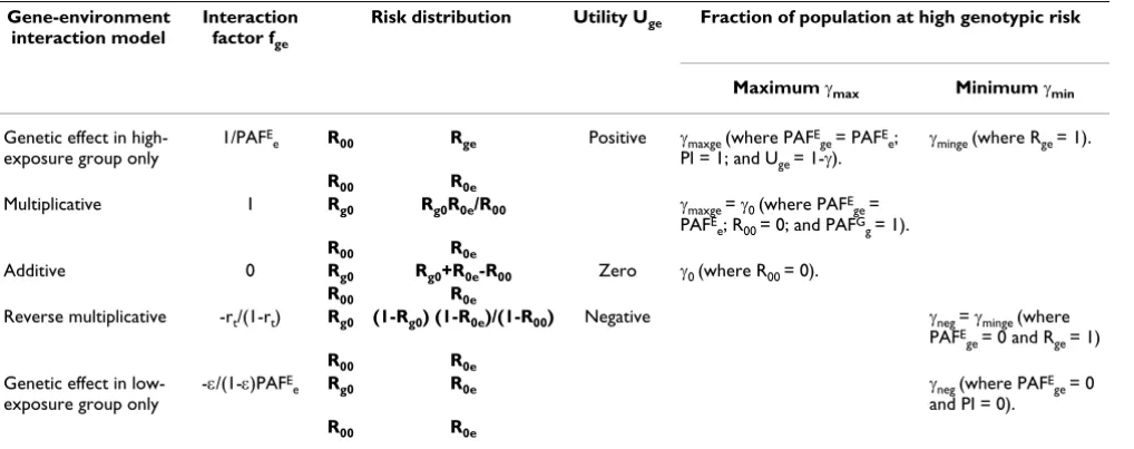
The full range of gene-environment interaction models specified by fge (within the limits given by Equation (48)) and the corresponding range of γ values are summarized in Table 4. Note that the risk distribution associated with f_ge = 1 corresponds to a multiplicative model of gene-envi-ronment interaction. If f_ge ≥ 1 solutions with population impact PI = 1 may exist (i.e. with PAFE

ge = PAFEe), pro-vided the proportion of the population in the high risk genotypic group takes the maximum value consistent with the data (γ = γmaxge). For lower values of fge, solutions with PI = 1 cannot exist.

One additional condition is necessary for solutions to exist, namely:

γ_max ≥γ_min (54)

This condition is always met if λ_MD ≤y_e + 1 (55)

where

and F1 and F2 are given by:

p R c

R c c R

g

DZ SD SD

MD SD MD SD

min

( )

( ) ( ) .

= −

− − −

{

1 1

}

( )

45

f

p

p

R p p

ge

g DZ

g DZ

DZ MD gtopDZ gDZ

2 1 1 46 = −         − −

( )

min (λ ) ( ) . p p

f R p

f R p

g DZ

g DZ

ge DZ MD gtopDZ

ge DZ MD gDZ

min min ( ) ( ) = + − + − 1 1 1 1 2 2 λ

λ

( )

447 .

−

− ≤ ≤

( )

ε ε

(1 )

1

48 PAF_eE fge PAF_eE

p_gDZ_min≤p_gDZ ≤p_gDZ_max

( )

49

p_gDZ_min≤p_gDZ ≤p_gnegDZ

( )

50

γ γ γ max max = ≥ ≤    

( )

ge ge ge f f for for 1 1 52 0 γ γ γ min min = ≥ −

(

−

)

≤ −

(

−

)

   

ge ge t t

neg ge t t

f r r

f r r

for

for

1

1

(( )

53

y

F f f

F F f r r

F f f

e

ge ge

ge t t

ge ge = ≥ ≥ ≥ −

(

−

)

− ≤ − 1 1 2 2 1 1 1 for for

for rr_t 1 r_t

56 −

(

)

     

( )

F r r PAF f PAF t t e E ge e 1 1 1 1 1 = −       − −            +  −    ε ε ε ε E E e t ge e t

r

r f r r

However, if λ_MD is greater than this, the requirement γ_max

≥γ_min further restricts the values of cSD that lie within the solution space (Table 3).

If V_e and ε are known, a solution space can be now be mapped for pDZ

g and fge with known input data from twin and sibling studies (λ_MZ, λ_DZ and λ_sib), for a given c_MD and all values of c_SD within the assumed range. The boundaries of the solution space are determined by the limits on f_ge given by Equation (48), the condition γmax ≥γmin (Equa-tion (54)), and the requirement that pDZ

g is less than or equal to 1/2 (Equation (20)) – no other condition on the genetic model is specified a priori. For each genetic risk model and gene-environment interaction model in the solution space, defined by pDZ

g and fge respectively, the variances V_g and V_ge can then be calculated, as can γ_max and

γ_min. For a chosen γ value in the allowed range, U_ge can then be calculated from Equation (28).

The model code is available as [Additional file 1: heritability12.xls].

Note that the condition on pDZ

g ≤ 1/2 may also be rewrit-ten using Equation (47), so that:

which is always met if

Before mapping the solution space, first consider some special cases and a comparison of the model with the clas-sical twin studies approach.

Special cases

1. No genetic variance

If V_g = 0, Equation (27) implies that V_ge = 0 also. Equations (29), (30) and (31) then give:

R_SD = c_SD (61)

and

R_MD = c_MD (62)

Under the usual assumption that c_MD = 1 (the 'equal envi-ronments' assumption), this is the well-known result that genetic variance can be zero only when the concordance in monozygotic and dizygotic twins is the same (leading to RMD = 1). However, if the equal environments assump-tion is not met (c_MD > 1), values of R_MD greater than 1 do not necessarily imply that a genetic component to the var-iance exists (see, for example, [18]).

2. No environmental variance

If V_e = 0, Equation (27) implies that V_ge = 0 also. Equations (29), (30) and (31) then give:

R_SD = 1 (63)

and

F

PAF

f PAF

eE

ge eE

2

1

1

58

=

(

−

)

−

(

)

( )

.

p

p

p R f p

g

DZ g

DZ

g

DZ MD e DZ gtop

DZ

≤ ⇒

−  



 ≤ ( − )

(

−

)

1 2

1 2

1 1 2 2

/

min

min

λ ( )559

p_gtopDZ ≤1 2/

( )

60 .

R_MD =1 p_gDZ

( )

64

Table 3: Further constraints on model parameters

Condition Limits on pDZ

g Limits on cSD

V_e ≥ 0

V_ge ≥ 0

Vg ≥ 0 CSD ≤RSD

γ_max ≥γ_min If λ_MD > y_e + 1 require: cSD ≥cSDm where p_gDZ ≤p_gtopDZ

p_gDZ ≥p_gDZ_min

c

R c f R y f c

SDm

DZ SD MD ge DZ MD e ge MD

= −1 ( − )( − ) + ( − ) + ( − )

1 1 1 1

1

2 2

λ λ

++ ( − )



For a purely genetic model with no environmental vari-ance, Equation (64) implies that if R_MD > 2, pDZ

g < 1/2. This is consistent with Risch's finding [16] that neither an additive genetic model nor a single dominant gene model (both with pDZ

g = 1/2) can fit the data for conditions such as schizophrenia (which has an R_MD value significantly greater than 2).

3. Classical twin study assumptions

Assuming no gene-environment interaction (V_ge = 0); an additive genetic risk model (pDZ

g = 1/2); and the 'equal environments' assumption (c_MD = 1) in Equations (29), (30) and (31) gives:

This is the classical twin study result, assuming the domi-nance term of the genetic variance is negligible. Note that, if R_MD = 2, the classical solution implies that the environ-mental variance terms in Equations (29) to (31) are zero and shared sibling risk is due to entirely to shared genes.

4. No correlation in genotypic risk in siblings (pDZ g = 0)

Equation (20) allows pDZ

g to tend to zero. Substituting pDZ

g = 0 in Equations (29), (30) and (31) and using the definition of the gene-environment interaction factor (Equation (28)) gives:

RSD = cSD (66)

and

Note that, from Equations (30) and (31), pDZ

g = 0 corre-sponds to a purely environmental explanation for shared sibling risks (although there may remain a genetic compo-nent to shared risks in monozygotic twins, from Equation (29)). The solution pDZ

g = 0 may not exist in reality; how-ever, the solution at this limit is of interest because low values of pDZ

g are plausible.

Also, note that if f_ge = 0 (no gene-environment interac-tion) and c_MD = 1 (the 'equal environments' assumption), the genetic variance V_g given by Equation (67) is half the classical twin study result (Equation (65)).

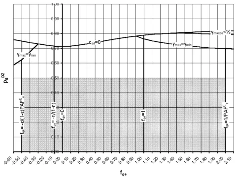
5. Cases where γ_max = γ_min

If the line γ_max = γ_min exists within the solution space, some special cases may arise with risk distributions of particular interest (including, for example, a solution with Rge = 1 and all other risks zero). These special cases and the con-ditions that they meet are shown in Table 5.

6. Cases where γmaxge < 1/2

Equation (27) shows that for a fixed gene-environment interaction factor f_ge and genetic variance component V_g, the utility U_ge is maximum when γ = 1/2, i.e. when half the population is in the high genotypic risk group, provided this solution exists. However, if γ_max < 1/2, utility is maxi-mum when γ = γ_max. As a smaller proportion of the popu-lation is then targeted, these solutions are of particular interest. Because solutions with population impact PI = 1 may exist when 1 ≤ fge ≤ 1/PAFEe if γ = γmaxge (Table 4), it is of interest to identify the area of the solution space with

V

r

g

t

MZ DZ

2 =2

(

λ −λ

)

( )

65

V

r

R c

f c

g

t

DZ MD MD

ge MD DZ

2 2

1

1 1

67

=

(

−

)

(

−

)

+

(

−

)



 

( )

λ

λ

Table 4: Limits on the gene-environment interaction factor (fge) and the proportion of the population in the high-genotypic risk group (γ).

Gene-environment interaction model

Interaction factor f_ge

Risk distribution Utility U_ge Fraction of population at high genotypic risk

Maximum γ_max Minimum γ_min

Genetic effect in high-exposure group only

1/PAFE

e R00 Rge Positive γmaxge (where PAFEge = PAFEe;

PI = 1; and Uge = 1-γ).

γminge (where Rge = 1).

R₀₀ R_0e

Multiplicative 1 R_g0 R_g0R_0e/R₀₀ γ_maxge = γ₀ (where PAFE

ge =

PAFE

e; R00 = 0; and PAFGg = 1).

R00 R0e

Additive 0 R_g0 R_g0+R_0e-R₀₀ Zero γ₀ (where R₀₀ = 0).

R₀₀ R_0e

Reverse multiplicative -rt/(1-rt) Rg0 (1-Rg0) (1-R0e)/(1-R00) Negative γneg = γminge (where

PAFE

ge = 0 and Rge = 1)

R₀₀ R_0e

Genetic effect in low-exposure group only

-ε/(1-ε)PAFE

e Rg0 R0e γneg (where PAFEge = 0

and PI = 0).

γ_maxge < 1/2. Maximum utility is then obtained when γ =

γ_maxge (where PI = 1 and U_ge = 1-γ_maxge). For the condition

where pDZ

gx is given by:

solving for pDZ

gx allows the region of the solution space where γmaxge < 1/2 to be defined.

7. Cases where the 'equal environments' assumption holds (c_MD = 1)

In the special case where the 'equal environments' assumption holds (c_MD = 1, and hence pDZ

gtop = 1/RMD), Equation (63) simplifies to give R_MD ≥ 2. Equation (62) also simplifies to give:

where

Meeting the condition pDZ

g ≤ 1/2 at cSD = 0 then requires:

It follows that if c_MD = 1, solutions with pDZ

g = 1/2 (an additive genetic model) and positive utility exist only when the following condition holds for R_MD:

Further, all three classical twin study assumptions (c_MD = 1, pDZ

g = 1/2 and fge = 0) can be met only for values of RMD that are low enough to satisfy:

1 + R_SD ≥R_MD > 1 (74).

If R_MD lies within this range, the classical twin study gives one possible solution; however, other solutions also exist. All alternative solutions favour a less 'genetic' and more 'environmental' explanation for shared sibling risks (i.e. they have higher values of c_SD). If R_MD is greater than 1+RSD, all three assumptions of the classical twin study cannot be met simultaneously.

Comparison with the classical twins approach

Table 6 summarizes the differences between the classical twin studies approach and the method adopted here.

A central feature of the model is that it abandons Fisher's assumption [26] that genes act as risk factors for common traits in a manner necessarily dominated by an additive polygenic term. In his historic 1918 paper, Fisher synthe-sized Mendelian inheritance with Darwin's theory of evo-lution by showing that the genetic variance of a continuous trait could be decomposed into additive and non-additive components [26,27]. Following Fisher, the classical twin study analysis depends on writing the genetic component of a trait as a convergent series of terms, consisting of an additive term (the sum of contri-butions of individual alleles at each locus) plus a smaller dominance term (the sum of contributions from pairs of alleles at each locus) and – usually neglected – epistatic terms (involving potentially multiple interactions between alleles at multiple loci) [15]. Often the additive term is assumed to dominate the series (equivalent to assuming pDZ

g = 1/2).

Fisher saw his polygenic model as "abandon [ing] the

strictly Mendelian mode of inheritance, and treat [ing]

Gal-ton's 'particulate inheritance' in almost its full generality" [26]. However, it can be argued that Fisher's model is flawed in so far as it fails to distinguish between the function of alle-les and the properties of traits [4,28]. In particular, epista-sis (although referred to here as 'gene-gene interaction') is not strictly an interaction between genes, but can be shown to depend on the structure and interdependence of metabolic pathways [28].

The alternative model adopted here is based on correla-tions in risk categories for a trait (which may be either envi-ronmental or genetic, or both), rather than single or multiple genetic variants. Adopting Porteous' critique [28], there is no a priori biological reason why the param-eter pDZ

g (the probability that the genotypic risk category of a dizygotic twin pair is identical by descent) cannot take any value between 1/2 (its value if the additive model holds) and zero. Low pDZ

g can then be understood to mean either a situation in which Fisher's polygenic model [26] is dominated by negative (synergistic) epistatic terms (for example, pDZ

g = 1/2n implies that interactions between n deleterious alleles are necessary to produce a phenotypic effect), or, more meaningfully, a situation in which human phenotypes are biologically robust to individ-ual genetic variants [29]. Thus, in the extreme case where numerous genetic variants combine to influence a trait through the interdependence of metabolic pathways, the trait may be highly correlated in monozygotic twins (who share all the genetic variants) but not correlated at all (pDZ

g = 0) in dizygotic twins or siblings (who share only γmaxge <1 2/ ⇒pgDZ >pgxDZ

( )

68

RMD(1−cSD)(pDZgx)2+[(1−cSD)(RMD− −1) (2cMD−1 1)(−RSD)]pDZgx −(RRSD−cSD)=0 ( )69

p_gDZ ≤1 2⇒c_SD≥c₁

( )

70

c

R f R

R f

SD ge DZ MD

MD ge DZ 1

2 2 1

1 1 1 2

2 1 1

= − −  + − − 

− _ + −

( ) ( )( )

( ) ( )

λ

λ 



( )

71

R R

f R

MD SD

ge DZ SD

≥ − −

+ −



 

( )

2 1

1 1

72

2

( )

( )

.

λ

R R

R PAF

MD SD

DZ SD eE

≤ − −

+ −



 

( )

2 1

1 1

73

2

( )

( ) /( )

Theoretical Biology and Medical Modelling

200

6,

3

:3

5

htt

p://

www.t

biomed.com/content/3/1/

Pag

e 12 of

(page number not for citation purposes)

models

Risk distribution Conditions Population

impact and Utility

Risk distribution Conditions Population

impact and Utility

Risk distribution Conditions Population impact and Utility

1 1 r_t = 1 PAF_e = 0 Undefined (PAF_ge = 0) R₀₀ 1 γ_minge = γ_maxge (R_ge = 1 and PAF_ge =

PAF_e) f_ge = 1/PAF_e

PI = 1 U_ge = 1-γ1 1

Rg0 1 γminge = γmaxge (Rge = 1 and PAFge = PAFe) fge ≥ 1

PI = 1 Uge = 1-γ R00 R00 0 1 rt = γε PAFe = 1 PI = 1 Uge = 1-γ

R₀₀ R₀₀ R_g0 1 γ_minge = γ₀ = γ_maxge (R_ge = 1; R₀₀ = 0; PAFge = PAFe) fge = 1

PI = 1 U_ge = 1-γ0 0

R_g0 1 γ_minge = γ₀ (R_ge = 1; R₀₀ = 0) 0 ≤ f_ge ≤ 1

0 = PI = 1 U_ge = PI-γ0 0 1 1 r_t = γ PAF_e = 0 Undefined (PAF_ge = 0)

0 R_0e 1-R_0e 1 γ_minge = γ₀ (R_ge = 1; R₀₀ = 0) f_ge = 0 PI = γ U_ge = 0 0 0

0 R0e 0 1 rt = ε PAFe = 1 PI = γ Uge = 0

0 1

Table 6: Comparison with classical twin study

Classical twin study Twins + siblings model

Genetic model Additive and dominance terms only: VDZ

g = 1/2VA+1/4VD Variable: VDZg = pDZgVg with 0 < = pDZg < = 1/2

Shared twin environments Equal environments assumption: cMD = 1 Variable: 1 < = cMD < = RMD cMD = RMD implies Vg = 0

Shared sibling environments Siblings not included. Variable: 0 < = c_SD < = R_SD Familial aggregation may be due to genes (c_SD

= 0) or environment (cSD = RSD).

Gene-environment interactions None Variable: V_ge = f2

ge· Vg· Ve/r2t -ε/(1-ε)PAFe < = fge < = 1/PAFe

Gene-environment correlations None None

Method Total phenoptypic variance given by: V_P = V_g+V_e V_P is input and a single solution for Ve and Vg calculated. Heritabilities are given by: H2 = Vg/VP h2 = VA/VP

half the relevant variants by descent). Although pDZ g = 0 may not be realistic, low values of pDZ

g are plausible, and may even be typical of complex diseases.

The classical twin study assumptions (see above) allow a single solution to be calculated from the under-deter-mined system of simultaneous Equations (29), (30) and (31). However, in the absence of prior knowledge about the form of the genetic model, the presence or absence of gene-environment interactions, and the validity of the 'equal environments' assumption, the approach adopted here is more rigorous.

Results

General model solutions

First consider the behaviour of the model when the 'equal environments' assumption holds and hence c_MD = 1 (as described above).

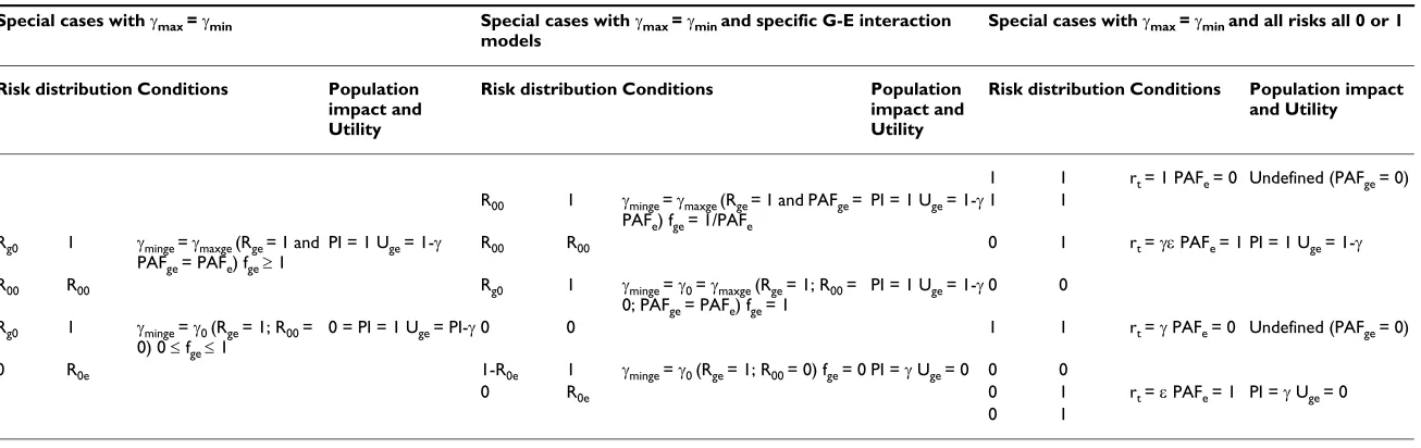
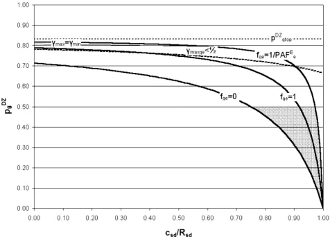
Figures 2, 3 and 4 show the possible solution spaces for an arbitrary set of plausible input parameters satisfying the requirement R_MD > 1+R_SD necessary for the classical twin study solution to exist. In Figure 2 the gene-environment interaction factor f_ge and hence utility, U_ge, are both posi-tive and in Figure 3 they are negaposi-tive. The horizontal axis shows cSD/RSD, which is zero if shared sibling risk is due to shared genetic factors only and 1 if shared sibling risk is due to shared environmental factors only. The vertical axis shows pDZ

g, which is 1/2 if the additive genetic model holds, but may reduce to zero if epistasis dominates and the phenotype is robust to genetic variation. The three curved solid lines represent three models of gene-environ-ment (G-E) interaction: an additive G-E model (i.e. no gene-environment interaction, f_ge = 0); a multiplicative G-E model (f_ge = 1); and maximum G-E interaction (f_ge = 1/ PAFE

e). The possible solution spaces are shaded grey. Each point in each shaded solution space corresponds to a

Example model solution space with RMD < 1+RSD and Uge ≥ 0

Figure 2

Example model solution space with R_MD < 1+R_SD and U_ge ≥ 0. Input parameters: λ_MZ = 3.4, λ_DZ = 3, λ_sib = 2, ε = 0.2,

PAFE

given genetic model (defined by pDZ

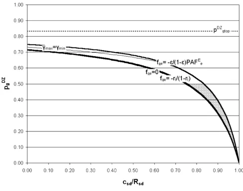
g) and a given G-E interaction model (defined by f_ge). Figure 4 plots the entire solution space (including both negative and posi-tive utility) by transforming the horizontal axis to repre-sent the G-E interaction parameter, f_ge. Although the classical twin model can fit the data, an infinite number of other solutions corresponding to different genetic and gene-environment interaction models also exist. In this example, the line γmax = γmin lies outside the solution space and no solutions exist with γ_maxge < 1/2.

For lower values of RMD, the curves defining the solution space are shifted downwards [see Additional files 2 to 9], so that the line fge = 0 (corresponding to no gene-environ-ment interaction) lies entirely below the line pDZg = 1/2 (corresponding to an additive genetic model). The classi-cal twin study solution does not exist, but many other

combinations of genetic and gene-environment interac-tion models may fit the data.

When cMD > 1, lines of constant fge no longer decrease monotonically to zero, and are also shifted upwards, so that solutions with strong G-E interactions are no longer possible [see Additional files 10 to 12].

Example applications using twin, sibling and environmental data

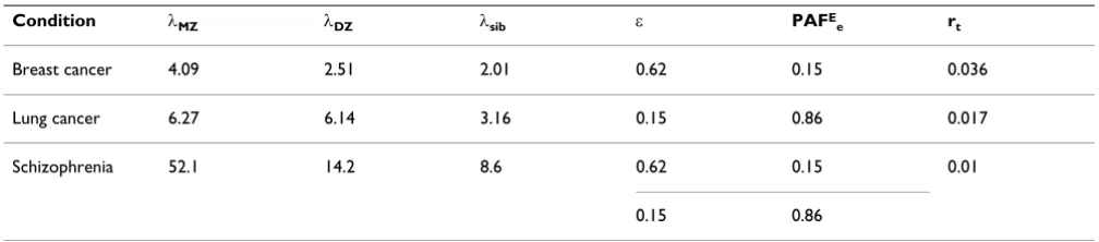
Input values

Consider example applications of the model for male lung cancer, female breast cancer and schizophrenia. The model input variables used are shown in Table 7.

The recurrence risks, λ, and total risks, r_t, for breast and lung cancer are those calculated by Risch [30], based on

Example model solution space with RMD < 1+RSD and Uge ≤ 0

Figure 3

Scandinavian twin data reported by Lichtenstein et al. [31] (involving more than 44,000 twin pairs) and Swed-ish familial data reported by Doug and Hemminki [32] (involving more than 2 million families). The proportion of the population exposed, ε, and population attributable fraction, PAFE

e, for breast cancer are taken from those reported by Rockhill et al. [33] for a US population. Although strictly speaking these values may not be appro-priate for a Scandinavian population, and include a com-ponent due to family history that may be (at least partly) genetic, they give a low V_e, consistent with the known environmental risk factors for breast cancer, and results are not sensitive to these input values (because V_e is so small). For lung cancer, it is assumed that 15% of the Scandinavian population smokes and that 86% of lung cancer cases could be avoided if they did not (giving a risk of lung cancer in smokers of 10%).

The recurrence risks λ, and total risk, rt, for schizophrenia are those used by Risch [16], based on European data summarized by McGue et al. [34]. More recent twin stud-ies for schizophrenia have given variable results and this example should be treated as illustrative only. Further, environmental exposures and population attributable fractions are unknown for schizophrenia. Two explora-tory sets of results are therefore reported, using data con-sistent with a low environmental variance (based on the values used for breast cancer), and high environmental variance (based on the values used for smoking and lung cancer).

Detailed results for the three diseases are shown in [Addi-tional file 13, 14, 15, 16, 17, 18, 19, 20, 21, 22, 23, 24, 25, 26, 27, 28, 29, 30, 31, 32, 33]. The key findings are out-lined below.

Example full model solution space with R_MD < 1+R_SD

Figure 4

Breast cancer results

For breast cancer, the PAFE

e associated with known envi-ronmental factors is low. The value of the model is there-fore less in calculating the utility of targeted environmental interventions than in exploring the solu-tion space for a complex disease with R_MD close to 2. Although strictly speaking the classical twin study solu-tion (with an additive genetic model, pDZ

g = 1/2, and an additive G-E model, fge = 0) does not exist as a solution, it might lie within the margin of error of the data. However, an infinite number of other models also could also fit the data. The classical twin model result always overestimates the genetic component of the variance, which reduces as the gene-environment interaction factor f_ge increases, and also as pDZ

g decreases (i.e. as epistatic terms begin to dom-inate the genetic model). These alternative models imply that shared environmental factors may partially explain familial aggregation of breast cancer. This contrasts with the classical twin method result (see earlier), which for R_MD = 2 leads to the inevitable conclusion that shared sib-ling risk must be due solely to shared genes [35].

In theory, a model with pDZ

g = 0 (where shared sibling risk is due entirely to shared environmental factors) could fit the data. However, for breast cancer the existence of known mutations that significantly increase risk (particu-larly mutations in the BRCA1 and BRCA2 genes, which are relatively common) rules out this solution. Although it is not possible to subtract out the effect of these mutations from the model, it is possible to show that they could be sufficient to explain the twin data if a G-E interaction also exists. For example, one possible solution consistent with the data could involve one or more dominant genes (pDZ

g = 1/2), a strong G-E interaction (f_ge = 1/PAFE

e), but a largely environmental explanation for shared sibling risk (say c_SD/R_SD = 0.9). This solution implies that the genetic component of the variance is less than a fifth of the classi-cal twin study result, which could be low enough to be explained by mutations in the BRCA1 and BRCA2 genes alone [35]. If this model were correct it would have important implications for women with such mutations,

but would not contribute significantly to reducing the incidence of breast cancer in the population as a whole, because the affected proportion of the population γ would be rather small. Other solutions, involving different genetic models with lower pDZ

g, and/or less gene-environ-ment interaction, are also possible.

The line γ_max = γ_min does not occur within the solution space for breast cancer; however, in some circumstances the lines γmax and γmin may be rather close together. This suggests that, although as expected there is always a trade-off between selecting a small proportion (γ_min) of the pop-ulation with a high Positive Predictive Value (PPV), or a larger proportion of the population (γ_max) with a higher Population Impact (PI) [19], some possible solutions could exist for breast cancer where the PPV and PI are both relatively high. Further, γ_max is often less than 1/2, so that, in these regions of the possible solution space, maximum utility might be obtained by targeting less than 50% of the population. However, known environmental factors for breast cancer are often not amenable to intervention and other possible solutions, with low, zero or negative utility, also exist.

Lung cancer results

For lung cancer, all the possible solutions imply that shared sibling risk is largely due to shared environmental factors (smoking) because solutions occur only when c_SD/ R_SD is close to 1. Unlike for breast cancer, the line γ_max =

γ_min lies outside the solution space, even for negative f_ge, as does the area of solutions with γmaxge < 1/2. However, the classical twin study solution, with f_ge = 0 and pDZ

g = 1/2, clearly lies within the solution space.

Although the classical twin model again provides an upper limit to the genetic component of the variance, even the classical result indicates that the risk of lung can-cer is dominated by smoking in this population and the variance has at most a small genetic component.

Unlike the breast cancer example, γ_max and γ_min are always far apart, suggesting a strong trade off between high Pos-Table 7: Input variables

Condition λMZ λDZ λsib ε PAFE

e rt

Breast cancer 4.09 2.51 2.01 0.62 0.15 0.036

Lung cancer 6.27 6.14 3.16 0.15 0.86 0.017

Schizophrenia 52.1 14.2 8.6 0.62 0.15 0.01

tive Predictive Value (R_ge) for a genotypic test and a high Population Impact (PI) for a targeted intervention. This means that a genotypic test that predicts which smokers will get lung cancer cannot exist. To predict all cases of lung cancer in smokers (i.e. to obtain PI = 1), 95% or more of the population would have to be in the high gen-otypic risk group, and the predictive value of such a test would be very low.

Because the genetic component of the variance is so small, it follows that the utility of genetic 'prediction and preven-tion' (measured by Uge) is also small (from Equation (28)). Utility is maximum when γ = 1/2, but even then values are low. The maximum utility of genotyping occurs when about 60% of cases could be prevented by targeting the 50% of smokers at high genotypic risk. However, other possible solutions have zero or negative utility.

Schizophrenia results

For schizophrenia, the classical twin study solution (with f_ge = 0 and pDZ

g = 1/2 and cMD = 1) cannot not fit the data. If the 'equal environments' assumption holds, neither a single dominant gene (pDZ

g = 1/2), nor additive polygenic model (also with pDZ

g = 1/2), nor single recessive gene (pDZ

g = 1/4) can explain the twin and family data, consist-ent with Risch's 1990 findings [16]. This may suggest that the genetic model for schizophrenia is likely to be domi-nated by epistatic terms. However, if gene-environment interactions are important, it is also possible that a reces-sive gene, combined with at least multiplicative G-E inter-action (pDZ

g = 1/4 and fge = 1 or higher), could explain the data.

The possible solution spaces include purely genetic expla-nations for shared sibling risk (at c_SD/R_SD = 0), or purely environmental ones (at c_SD/R_SD = 1, applicable if pDZ

g = 0). Assuming a small environmental component to the vari-ance, there is no region of the solution space for which

γ_maxge < 1/2, suggesting that the utility of targeted environ-mental interventions under these assumptions is likely to be low. However, if the environmental component of the variance is assumed to be much larger, the available solu-tion space changes dramatically, because the line γmax =

γ_min now constrains the solution space to a much smaller area, which excludes solutions with no G-E interaction (f_ge = 0). Special solutions may exist along the line γmax = γmin, as shown in Table 5. Because the environmental factors contributing to schizophrenia are unknown, it is impossi-ble to draw any conclusions about the potential benefits of targeting environmental interventions at those at high genotypic risk.

Because prenatal development is thought to be important in schizophrenia, it is plausible that monozygotic twins

are more likely to share environmental risk factors than dizygotic twins are. Breaking the 'equal environments' assumption changes the shape of the solution space sig-nificantly, and, assuming a small environmental compo-nent to the variance, only limited G-E interactions are now possible (the multiplicative G-E model, f_ge = 1, lies largely outside the solution space). The utility of targeting environmental interventions by genotype is then likely to be low. However, in these circumstances it is possible that an additive genetic model (pDZ

g = 1/2) with some G-E interaction, or a recessive gene (pDZ

g = 1/4) with no G-E interaction, could explain the data.

Discussion

If Fisher's polygenic model [26] is abandoned, along with the usual twin study assumption that there are no gene-environment interactions, the four-category model devel-oped by Khoury and others can be combined with twin, family and environmental data to implement a 'top down' approach to assessing the utility of targeting environmen-tal/lifestyle interventions by genotype. Scoping studies, valid when R_SD ≠ 1, provide a first step to modelling the health of populations [23].

Abandoning Fisher's assumption that the polygenic model is necessarily dominated by an additive term can be justified by the growing evidence that phenotypic effects can result from the synergistic action of alleles in many genes [36]. For example, Bardet-Biedl Syndrome, historically assumed to be a recessive trait, has been shown to involve three interacting mutations at two loci in some patients (implying that pDZ

g = 1/8) and, more recently, an additional locus has been identified that can also interact to change disease severity and symptoms [37]. Both positive and negative gene-environment inter-actions have also been observed in human diseases, although there are difficulties in confirming their statisti-cal validity [38,39].

The model also allows the impact of the much criticised 'equal environments' assumption to be explored.

A number of conclusions can be drawn about the merits of the classical twin study and the utility of genetic 'predic-tion and preven'predic-tion'.

generalizes Risch's findings [16] to show that the three assumptions of the classical twin model cannot all be sat-isfied simultaneously. For intermediate R_MD values, observed for conditions such as breast cancer (for which R_MD is approximately 2), the model illustrates that the conclusion drawn from classical twin studies, that familial aggregation is due entirely to shared genetic factors, may be erroneous. This raises the possibility – previously rejected on the basis of twin study results [35] – that genetic variants are important in determining risk only for the relatively rare familial forms of cancer. If so, genetic models of familial aggregation (for example [40]) may be incorrect and the hunt for additional susceptibility genes could be largely fruitless. Existing published findings might then reflect prevailing bias, rather than true associ-ations [14].

Secondly, the model confirms that the potential for reduc-ing the incidence of common diseases usreduc-ing environmen-tal/lifestyle interventions targeted by genotype may be limited [7] by:

(i) the low importance of genetic differences in determin-ing the risk of some conditions (for example, lung can-cer);

(ii) the complexity of gene-gene and gene-environment interactions and/or lack of knowledge of environmental factors (for example, schizophrenia).

Targeting environmental/lifestyle interventions at those at 'high genotypic risk' can be of high utility only in specific circumstances. The utility of targeting environmental interactions by genotype (compared to randomly select-ing the same number of people from the population) is zero if there is no gene-environment interaction. Utility can also be negative in the presence of a negative interac-tion (i.e. if the people at high genotypic risk have less to

gain by the intervention than people at low genotypic

risk). The finding that utility increases with gene-environ-ment interaction is consistent with Khoury and Wagener [19] but the relationship is considerably clarified by the adoption here of different measures of the population attributable fraction associated with a targeted interven-tion (PAFE

ge) and of utility (Uge). Further, by formally introducing constraints on the model (for example, that risks are positive and do not exceed 100%), it is possible to demonstrate that both the gene-environment interac-tion factor and utility have maximum values, which can-not be exceeded for a given data set.

The lung cancer example is apparently trivial but also of critical importance. The R_MD value for lung cancer is close to 1, and neither the Scandinavian data used here [31], nor earlier US studies [41], have identified a significant

heritable component. It follows from Equation (27) that if the genetic component of the variance, V_g, is zero, V_ge (the G-E component of the variance) is also zero and using genotyping to target an intervention such as smok-ing cessation is therefore of zero utility (no better than randomly selecting the same number of individuals). This approximate conclusion is confirmed by the results pre-sented for lung cancer, which show extremely low utility. The detailed calculations may at first sight seem unneces-sary, particularly because smoking causes multiple dis-eases and targeting smoking cessation on the basis of lung cancer risk alone is therefore ill-advised. However, the idea that a genetic test will one day predict which smokers get lung cancer has been widely promoted in the literature and has driven much research aimed at identifying the supposed 'genes for lung cancer' [42]. The results pre-sented here strongly suggest that there will never be a genetic or genotypic test that predicts which smokers will get lung cancer, because the genetic component of the var-iance is not high enough.

Finally, the model illustrates the argument of Terwilliger and Weiss [11] that the potential for population biobanks to quantify risks for complex disease is limited by a 'mul-tiple testing' problem caused by the large number of genetic and gene-environment interaction models that could fit existing data. Each point in each solution space described above represents a different combination of a genetic risk model (defined by pDZ

g) and a G-E interaction model (defined by f_ge). Further, any given value of pDZ

g may be obtained by an infinite number of different com-binations of different alleles acting through multiple bio-logical pathways. Because the number of hypotheses that could be tested is essentially infinite, sample sizes neces-sary to quantify the risks (R_oo, R_go, R_oe and R_ge) could

"plausibly be larger than the number of people that have ever lived" [11].

the extent to which environments are correlated between different types of relative.

Treating exposure and environmental variance (or popu-lation attributable fraction) as input data is also problem-atic when the effects of environmental factors on risk are often unknown. Further, the simple nature of the model (with one environmental axis) cannot adequately repre-sent the complexity of environmental (including socio-economic) causes of disease. However, if targeting envi-ronmental interventions by genotype is to be considered, this implies that at least something is known (or expected to be learned) about environmental factors, such as partic-ular exposures, that are amenable to intervention.

The assumption of no gene-environment correlation will often hold (for example it is rather implausible that the same genes strongly influence both lung cancer risk and nicotine addiction), but is not necessarily always true. Adult lactose intolerance is an example of a condition with a strong gene-environment interaction where tar-geted intervention to avoid drinking milk may be of high utility. However, the model is invalid for lactose intoler-ance unless exposures are applied equally to the popula-tion studied because, in general, people who are lactose intolerant may be less likely to drink milk (a gene-envi-ronment correlation) owing to the unpleasant symptoms.

A more fundamental problem is caused by the assump-tions that: (i) the risks R_oo, R_go, R_oe and R_ge are inherent properties of a given trait within a given population (with a given γ and ε) and that there are therefore no confound-ers; and (ii) risks are randomly distributed within these categories.

These assumptions, although often made, are implausible in many situations. The assumption of no confounders means that the model can only represent a subset of the potential models of gene-gene and gene-environment interaction described by more complex models (for exam-ple [17]). It is unlikely to be met if multiexam-ple genetic factors interact with multiple environmental ones [44]. Although this may well render the results presented here invalid, such complexity is likely to reduce the utility of targeting by genotype, rather than enhance it. Hence, situations where the 'no confounders' assumption at least approxi-mately holds are those most likely to be of relevance to public health.

The second assumption neglects the fact that for most exposures there is a gradient in risk, with higher exposure meaning higher risk, and that the same may also be true of genetic factors. This means that increasing the number of categories in the model will increase V_e (see [45]) and perhaps Vg. Further, these subcategories may be

differ-ently correlated between relatives (for example, the twin of a heavy smoker may be more likely to be a heavy smoker than a light one). If so, a relative of a proband may not be representative of their allocated risk category in the four-