Stratified Random Sampling
Rajesh Singh
Department of Statistics B.H.U., Varanasi (U.P.) India
Mukesh Kumar
Department of Statistics B.H.U., Varanasi (U.P.) India
Manoj K. Chaudhary
Department of Statistics B.H.U., Varanasi (U.P.) India
Cem Kadilar
Department of Statistics Hacettepe University Beytepe 06800, Ankara Turkey
Abstract
In this article we have considered the problem of estimating the population mean
Y in the stratified random sampling using the information of an auxiliary variable x which is correlated with y and suggested improved exponential ratio estimators in the stratified random sampling. The mean square error (MSE) equations for the proposed estimators have been derived and it is shown that the proposed estimators under optimum condition performs better than estimators suggested by Singh et al. (2008). Theoretical and empirical findings are encouraging and support the soundness of the proposed estimators for mean estimation.Keywords: Auxiliary variable, exponential ratio-type estimates, mean square error, stratified random sampling.
2000 AMS Classification: 62D05
1. Introduction
such as Upadhayaya and Singh (1999), Sisodia and Dwivedi (1981), Singh and Tailor (2003), Singh et al. (2007), developed various estimators to improve the ratio estimators in the simple random sampling. Kadilar and Cingi (2003) adapted the estimators in Upadhyaya and Singh (1999) to the stratified random sampling.
In this study, under stratified random sampling without replacement scheme, we suggest two improved exponential estimators which are more efficient than estimators proposed by Singh et al. (2008). There are some recent studies proposing the family of estimators without using the exponential function in literature, such as Koyuncu and Kadilar (2009(a,b)), Khoshnevisan et al. (2007), Singh and Vishwakarma (2006, 2008) etc. However, in this article, the proposed family of estimators depends on the exponential function.
We assume that the population comprises N units, which can be uniquely
partitioned into L strata of size N1, N2,…, NL such that
L
1
h h
. N
N The strata
weights Wh= Nh/ N (h=1, 2,…, L) are assumed known. Let (yhi, xhi) (i=1, 2,…, Nh)
denote the values of variates (y, x) respectively for the i-th unit in the h-th stratum and Yhand Xh denote stratum means.
When the population mean of the auxiliary variable, X, is known, Hansen et al. (1946) suggested a combined ratio estimator for estimating the population mean of the study variable
Y :X x y t
st st
1 , (1.1)
where L h
1
h h
st w y
y
, h
L 1
h h
st w x
x
, and X w Xh.
L 1
h h
Here
nh
1
i hi
h
h y
n 1
y , and
nh
1
i hi
h
h x
n 1
x .
The MSE of t1to a first degree of approximation is given by
L
1 h
yxh 2
xh 2 2 yh h 2 h
1 w S R S 2RS
t
MSE , (1.2)
where
h h h
N 1 n
1 ,
st st
X Y X Y
R is the population ratio, S2yh is the
population variance of a study variable, S2xh is the population variance of the
auxiliary variable and Syxh is the population covariance between study and
2. Kadilar and Cingi estimator
Kadilar and Cingi (2003) introduced an estimator for population mean using known value of some population parameters in stratified random sampling given by
2
t
= st,a,bb , a , st
st X
x y
(2.1)
where
h h
L
1 h
h h b
, a ,
st w a x b
x
,
h h
L 1 h
h h b
, a ,
st w a X b
X
and ah, bh are the
functions of the known parameters of the auxiliary variable such as coefficient of variation Cxh, coefficient of kurtosis 2h(x)etc., or some constants in the hth
stratum .
The MSE of the estimator t2is given by
MSE(
t
2 ) =
L
1 h
h 2 h
W
a,b h yxh
2 xh 2 h 2
b , a 2
yh R a S 2R a S
S , (2.2)
where .
X Y R
b , a , st
st b
,
a
Bahl and Tuteja (1991) suggested an exponential ratio type estimator for population mean in simple random sampling as
x
X
x
X
exp
y
t
3 . (2.3)Motivated by Bahl and Tuteja (1991), Singh et al. (2008) adapted this estimator to the stratified random sampling as
i 4 i 4
i 4 i 4 st
i 4
x X
x X exp y
t , i = 0, 1, 2, 3, 4. (2.4)
where
h L
1 h
h
40 w x
x
, X Lw Xh,
1
h h
40
h xh
L
1 h
h
41 w x C
x
,
h xh
L
1 h
h
41 w X C
X
,
x (x)
w
x h 2h
L
1 h
h 42
, X w
Xh 2h(x)
L
1 h
h 42
,
h 2h xh
L
1 h
h
43 w x (x) C
x
,
h 2h xh
L
1 h
h
43 w X (x) C
X
,
x C (x)
w x
L
, X w
X C (x)
L
The bias and MSE of the estimators t4i ( i=0,1,2,3,4) can be obtained respectively
by following expressions:
L 1 h yxh hi 2 xh 2 hi i 4 h 2 h i 4 i4 a S
2 1 S a R 8 3 w X 1 ) t (
Bias , (i=01,2,3,4) (2.5)
L 1 h 2 xh 2 hi 2 i 4 yxh hi i 4 2 yh h 2 h i4 a S
4 R S a R S w ) t (
MSE , (i=01,2,3,4) (2.6)
where, , X w Y R h L 1 h h st 40 , ) C X ( w Y R L 1
h h h xh
st 41 , )) x ( X ( w Y R L 1
h h h 2h
st 42 , ) C ) x ( X ( w Y R L 1
h h h 2h xh
st 43 , )) x ( C X ( w Y R L 1
h h h xh 2h
st 44 . Y Y w Y L 1
h h h
st
We would like to remark that for various values of parameters in (2.4), we get five estimators (for I = 0, 1, 2, 3, 4) as shown in Table 1. The MSE expressions for these estimators are also given in the Table 1.
Table 1: Some members of family of estimators t4i
The values
of ah,bh Estimator MSE of the Estimator
ah=1, bh=0
st st st 40 x X x X exp y t
2 xh 2 40 yxh 40 2 yh h L 1 h 2h 4 S
R S R S w
ah=1,
bh=Cxh
41 41 41 41 st 41 x X x X exp y t
2 xh 2 41 yxh 41 2 yh h L 1 h 2h 4 S
R S R S w
ah=1,
bh=2h(x)
42 42 42 42 st 42 x X x X exp y
t
2 xh 2 42 yxh 42 2 yh h L 1 h 2h
4
S
R
S
R
S
w
ah=2h(x),
bh=Cxh
43 43 43 43 st 43 x X x X exp y
t
L 1 h 2 xh 2 h 2 2 43 yxh h 2 43 2 yh h 2
h 4 (x)S
R S x R S w
ah=Cxh,,
bh=2h(x)
44 44 44 44 st 44 x X x X exp y t
L 1 h 2 xh 2 xh 2 44 yxh xh 44 2 yh h 2h 4 C S
Remark 1 - Here we would like to mention that the choice of the estimator depends on the availability and values of the various parameter(s) used (for choice of the parameters ah and bh refer to Singh et al. (2008) and Singh and
Kumar(2009)).
Singh et al. (2008) showed that all of these modified estimators (t4i) have a
smaller MSE than the MSE of the stratified version of exponential ratio type estimator t3st under certain conditions:
st st st
st 3
x X
x X exp y
t (2.7)
Note that t3stis the same estimator with t40.
Singh et al. (2008) reported the minimum value of mean square error of the
estimator t4i asMSE(t ) w S2yh(1 2c) L
1 i
h 2 h min
i
4
(2.8)
where, c is combined correlation coefficient in stratified sampling across all
strata. It is calculated as .
S w S
w
S S w
L
1 1
L
1 i
2 xh h 2 h 2
yh h 2 h
2 L
1 i
xh yh h h 2 h 2
c
3. Suggested modified exponential ratio estimator
In stratified random sampling, Kadilar and Cingi (2005) introduced a ratio estimator as
1 5 kt
t , (3.1)
where the constant k is obtained by minimizing the MSE of t5.
Motivated by Kadilar and Cingi (2005), we propose the following modified estimator
i 4 i 6 kt
t
i 4 i 4
i 4 i 4 st
x X
x X exp y
k , i = 0, 1, 2, 3, 4. (3.2)
To obtain the MSE of t6i to the first degree of approximation, let us define
* i
* i * i *
i 1 st
0
A A a e and Y
Y y
e . Using these notations we have
0
st Y1 e
where
L 1 h h hi h *i w a X
A , a Lw a x ,
1
h h hi h
*
i
e E
e 0 E 0 1i* ,
2yh L 1 h h 2 h 2 2
0 w S
Y 1 e E
,
2xh L 1 h hi h 2 h 2 * i 2 i
1 w a S
A 1 e E
,
yxhL 1 h hi h 2 h * i * i 1
0 w a S
A Y 1 e e E
.Expressing (3.2) in terms of e’s, we have
1 * i 1 * * i 1 * 0 i i 6 2 e 1 2 e exp e 1 Y k t 2 e e 8 e 3θ 2 e e 1 Y k * i 1 0 * 2 * 1i 2 * * i 1 * 0i . (3.3)
where i 4 * i * i X A . ) Y (t E ) (t
Bias 6i 6i
) 2 ) ee ( E 8 ) e ( E 3 ( Y k ) 1 k ( Y * i 1 * i 2 * i 1 * i st i i st
hi yxh
2 xh 2 hi i 4 L 1 h h 2 h i 4 i i
st a S
2 1 S a R 8 3 w X k ) 1 k ( Y ) t ( Bias k ) 1 k (
Yst i i 4i
(3.4)
From (3.3), we have
2 xh 2 hi 2 i 4 yxh hi i 4 2 yh L 1 h h 2 h 2 i 2 2 i i6 a S
4 R S a R S w k Y 1 k ) t ( MSE
4i hi yxh
2 xh 2 hi 2 i 4 L 1 h h 2 h i
i R a S
2 1 S a R 8 3 w ) 1 k ( k
MSE of the estimator t6i can be rewritten as
t6i ki 1
2Y2 ki2MSE
t4i 2ki
ki 1
YstBias
t4iMSE (3.6)
To obtain the optimum value of k, we partially differentiate the expression (3.6) with respect to k and put it equal to zero as follows:
t 0 MSEk 6i
,
k MSE t (k 1) Y 2k (k 1)Y Bias(t )
0k i i st 4i
2 2 i i 4
2
,
4i i 2i 2 *
i
A 2 t MSE Y
A Y k
, i = 0, 1, 2, 3, 4. (3.7)
where
. S a R 2 1 S a R 8 3 w
) (t Bias Y
A 24i 2hi 2xh 4i hi yxh
L
1 h
h 2 h 4i
st
i
Note that 0< * i
k <1.
Remark 2
Shahbaz and Hanif (2009) proposed a general class of shrinkage estimator in survey sampling as
) t
ˆ
( MSE T
1 t
ˆ
t
ˆ
2
s
(3.8)
where tˆ is any available estimator of parameter T. The minimum MSE of tˆs reported by Shahbaz and Hanif (2009) as
) t
ˆ
( MSE T
1
) t
ˆ
( MSE )
t
ˆ
( MSE
2
s
(3.9)
Following Shahbaz and Hanif (2009), the estimator t6iis written as
, ) t
ˆ
( MSE Y
1
t
ˆ
t
ˆ
i 4 2
i 4 iS
6
i=0,1,2,3,4. (3.10)
and the minimum MSE of tˆ6iSis given by
) t
ˆ
( MSE Y
1
) t
ˆ
( MSE )
t ( MSE
i 4 2
i 4 iS
6
4. Improved estimator
We propose classes of estimators for estimating the population mean
Y , in the stratified random sampling as,
t
y
t
7i
1i st
2i 4i i = 0, 1, 2, 3, 4.
i 4 i 4
i 4 i 4 st
i 2 st i 1
x
X
x
X
exp
y
y
. (4.1)where 1i and 2i are real constants. There are two choices in terms of how to
select 1i and 2i. Some authors, such as Kadilar and Cingi (2006), use the
constraint 1i + 2i = 1, while others use an unconstrained selection of 1i and
2i. This latter group includes Upadhyaya et al. (1985), Singh et al. (1988) and
Shabbir and Gupta (2207). These authors choose 1iand 2iwhich minimize the
MSE for the proposed estimator and do not insist on having 1i + 2i = 1.
In this paper we have made unconstrained selection of 1iand2i.
Expressing (4.1) in terms of e’s by using the same notations as defined earlier we have
1 i 1 * i 0
* i i
2 0 i
1 i 7
2 e 1 2
e exp Y )
e 1 ( Y
t (4.2)
Expanding the right hand side of (4.2), and retaining the terms to the first order of approximation, we have
2 e e 8
e 3 2
e e
1 Y )
e 1 ( Y t
* i 1 0 * i 2 *
i 1 2 * i *
i 1 * i 0 i
2 0 i
1 i
7 (4.3)
The bias of the estimator t7i , to the first order of approximation, is obtained as
) Y t ( E ) (t
Bias 7i 7i
4i hi yxh
2 xh 2 hi 2
i 4 L
1 h
h 2 h i 2 st i
2 i
1 R a S
2 1 S a R 8 3 w
Y ) 1 (
) t ( Bias Y Y
) 1
(1i`2i st 2i st 4i
(4.4)
From equation (4.4), we observe that to the first order of approximation the proposed estimator is biased.
From (4.3), squaring and than retaining the terms of e’s upto power two, we have
2i 7 i
7 ) E t Y
t (
MSE
i i 2 st i
2 ` i
1 1)Y A
(
2 st * i 1 0 * i 2 * i 1 2 * i * i 1 * i 0 i 2 0 i 1 Y 2 e e 8 e 3 2 e e 1 Y ) e 1 ( Y E 2 * i 1 0 * i 2 * i 1 2 * i * i 1 * i 0 i 2 0 i 1 i 2 i 1 2 e e 8 e 3 2 e e Y Y e ) 1 ( Y E
1
D MSE(t ) Y2 1i 2i 2 12i 22i 4i
i1 2i
2i i ii 2 i
1 C 2 1 A
2
(4.5) where
hi yxh
i 4 2 yh L 1 h h 2 h
i a S
2 R S w
C and L h 2yh
1 h
2 h S
w
D
.
In order to find optimum value of estimator t7i, we differentiate MSE (t7i) with
respect to 1i and 2i. The optimum values of 1i and2i are
4i i
2 2 2 i i 2 i i 4 2 2 i i 2 i 2 * i 1 A 2 ) t ( MSE Y D Y A C Y A 2 ) t ( MSE Y Y A C Y A Y (4.6) and
4i i
2 2 2 i i 2 i 2 2 2 i i 2 * i 2 A 2 ) t ( MSE Y ) D Y ( ) A C Y ( ) A Y )( D Y ( Y ) C A Y (
. (4.7)
Using these optimum values, * i 1
and *
i 2
, in the place of 1iand 2i in (4.5), respectively, we get the minimum MSE of the estimator t7i.
Remark 3 - Here we would like to mention that the optimum values of 1iand i
2
5. Efficiency comparisons
For the estimators, efficiency comparisons are given below.
In this section, we first compare modified estimator t6i given in (3.2), with the
estimator t4igiven in (2.4).
MSE (t6i) < MSE (t4i), i = 0, 1, 2, 3, 4,
2 yxh 2 h 2
i 4 yxh h i 4 2 yh L
1 h
h 2 h 2 i 2 2
i a S
4 R S
a R S w
k Y 1 k
4i hi xyh
2 xh 2 hi 2
i 4 l
1 h
h 2 h i
i R a S
2 1 S a 8 R 3 w ) 1 k ( k 2
2 xh 2 hi 2
i 4 yxh hi i 4 2
yh h L
1 h
2
h
4
a
S
R
S
a
R
S
w
,i i
4 2
i 4 2
i
A 2 ) t ( MSE Y
) t ( MSE Y
k
. (5.1)
As the condition (5.1) is always satisfied, we can say that the suggested estimator is more efficient than exponential ratio estimator in stratified random sampling in all conditions. Note that when i = 0, MSE (t40) = MSE (t3st).
Second, we compare the improved estimator t7i, given in (4.1), with estimator t4i,
given in (2.4) as follows:
MSE (t7i) < MSE (t4i), i = 0, 1, 2, 3, 4,
2 4i 1i 2i i
1i 2i
2i iii 2 2
i 1 2 i 2 i 1
2 1 D MSE(t ) 2 C 2 1 A
Y
2 xh 2 hi 2
i 4 yxh hi i 4 2
yh h L
1 h
2
h
4
a
S
R
S
a
R
S
w
.Let (1i 2i 1)Bi. Then the expressions can be obtained on solving as
* i 3
* i 2 *
i 1 2 Y
, (5.2)
where
2
i 2 i4 *
i
1 MSEt 1
,
2 1i 2i ii 1 i i 2 i *
i
2 2A B D2 C
,
2 *
B
Next, we compare the improved estimator t7i given in (4.1) with the estimator t6i
given in (3.2).
MSE (t7i) < MSE (t6i), i = 0, 1, 2, 3, 4,
2 4i 1i 2i i
1i 2i
2i ii 2 2
i 1 2 i 2 i 1
2 1 D MSE(t ) 2 C 2 1 A
Y
4i hi xyh
2 xh 2 hi 2
i 4 l
1 h
h 2 h i
i i 4 2
i 2 i 2
S a R 2 1 S a 8 R 3 w
) 1 k ( k 2 t MSE k 1 k
Y ,
i 3
i 2 i 1 2 Y
, (5.3)
where
2
i 2 2 i i 4 i
1 MSE t k
,
2 1i 2i ii 1 i
2 i
i i i
2 2A k k 1 B D2 C
,
2 i 2 i i3 B k 1
.
Finally, we compare the improved estimator t7i, given in (4.1), with
estimatorMSE(t4i)min given in (2.8).
min i 4 i
7 ) MSE(t )
t (
MSE , i = 0, 1, 2, 3, 4,
). 1 ( S w
A 1 2
C 2
) t ( MSE D
1 Y
2 c L
1 h
2 yh h 2 h
i i 2 i
2 i 1 i
i 2 i 1 i
4 2
i 2 2
i 1 2 i 2 i 1 2
or
* i 3
* i 2 *
i 1 * 2 Y
(5.4)
where,
min i 4 *
) t ( MSE
2 i 2 i 4 *i
1 MSEt
,
2 1i 2i iii 1 i i 2 i *
i
2 2A B D2 C
,
2 i i *
3 B
In all above expressions we used optimum values of 1i, 2i , andki, i.e.,
* i 1 i 1
, 2i *2i, and ki= * i
k , respectively.
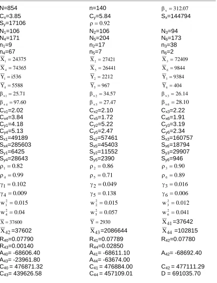
Table 2: Data Statistics
N=854 n=140 x 312.07
Cx=3.85 Cy=5.84 Sx=144794
Sy=17106 0.92
N1=106 N2=106 N3=94
N4=171 N5=204 N6=173
n1=9 n2=17 n3=38
n4=67 n5=7 n6=2
24375
X1 X2 27421 X3 72409
74365
X4 X5 26441 X6 9844
536 i
Y1 Y2 2212 Y3 9384
5588
Y4 Y5 967 Y6 404
71 . 25 1 x
x2 34.57 x3 26.14
60 . 97 4 x
x5 27.47 x6 28.10
Cx1=2.02 Cx2=2.10 Cx3=2.22
Cx4=3.84 Cx5=1.72 Cx6=1.91
Cy1=4.18 Cy2=5.22 Cy3=3.19
Cy4=5.13 Cy5=2.47 Cy6=2.34
Sx1=49189 Sx2=57461 Sx3=160757
Sx4=285603 Sx5=45403 Sx6=18794
Sy1=6425 Sy2=11552 Sy3=29907
Sy4=28643 Sy5=2390 Sy6=946
82 . 0
1
2 0.86 3 0.90
99 . 0
4
5 0.71 6 0.89
102 . 0 1
2 0.049 3 0.016
009 . 0 4
5 0.138 6 0.006
015 . 0
w12 w22 0.015 w23 0.012
04 . 0
w24 w 0.057
2
5 w 0.041
2 6
37600
X Y2930 X41=37642
42
X =37602 X43=2086644 X44 =102815
R40=0.07790 R41=0.07789 R42=0.07780
R43=0.00140 R44=0.02850
A40= -68606.40 A41= -68611.10 A42= -68692.40
A43= -23961.80 A44= -63674.00
C40= 476871.32 C41= 476884.00 C42= 477111.29
6. Numerical study
For empirical study, we use the data set earlier presented by Kadilar and Cingi (2003). In this data set, Y is the apple production amount and X is the number of apple trees in 854 villages of Turkey in 1999. The population information about this data set is given in Table 2.
By using this data, we have calculated MSE values of suggested estimators and compared them with MSE values of Singh et al. (2008) estimators. For the different values of ah and bh, we can find the MSE equations of all members of
the improved estimator t7i by simply changingR4i, respectively.
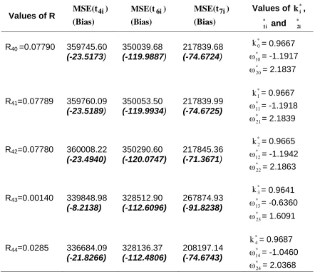
Table 3: MSE Values of Estimators
Values of R
(Bias) ) MSE(t4i
(Bias) ) MSE(t6i
(Bias) )
MSE(t7i Values of * i
k , *
1i
ω and ω*2i
R40=0.07790 359745.60 (-23.5173)
350039.68
(-119.9887)
217839.68
(-74.6724)
* 0
k = 0.9667
* 10
= -1.1917
* 20
= 2.1837
R41=0.07789 359760.09 (-23.5189)
350053.50
(-119.9934)
217839.99
(-74.6725)
* 1
k = 0.9667
* 11
= -1.1918
* 21
= 2.1839
R42=0.07780 360008.22 (-23.4940)
350290.60
(-120.0747)
217845.36
(-71.3671)
* 2
k = 0.9665
* 12
= -1.1942
* 22
= 2.1863
R43=0.00140 339848.98 (-8.2138)
328512.90
(-112.6096)
267874.93
(-91.8238)
* 3
k = 0.9641
* 13
= -0.6360
* 23
= 1.6091
R44=0.0285 336684.09 (-21.8266)
328136.37
(-112.4806)
208197.14
(-74.6743)
* 4
k = 0.9687
* 14
= -1.0460
* 24
= 2.0368
under optimum conditions performs better than all other estimators proposed by Singh et al. (2008). We also observe from the table that the estimator t73 is
having larger MSE than the minimum MSE attained by Singh et al. (2008). So, for this data set choice of ah=2h(x) and bh=Cxh is not a good choice. Also, for the
choice ah=Cxh and bh= 2h(x) the MSEs of the estimators t44, t64 and t74 is
minimum.
7. Conclusion
As shown in theory, we also observe from Table 3 that suggested estimators t6i
(including optimal value) performs better than corresponding estimators without optimal values, t4i. Besides, we see that improved estimator t7i and its members
are always more efficient than corresponding estimators (without optimal value of kiand with k*i) for this data set.
Acknowledgements
The authors are thankful to the referee for his valuable comments and suggestions regarding the improvement of the paper. The second author (Mukesh Kumar) is grateful to UGC, New Delhi, India, for providing financial assistance.
References
1. Bahl, S. and Tuteja, R.K. (1991). Ratio and product type exponential estimator. Information and Optimization Science XIII 159-163.
2. Hansen, M.H., Hurwitz, W.N. and Gurney, M. (1946). Problem and methods of the sample survey of business. Journal of American Statistical Association 41 174-189.
3. Kadilar, C. and Cingi, H. (2003). Ratio estimators in stratified random sampling, Biometrical Journal 45 (2), 218-225.
4. Kadilar, C. and Cingi, H. (2005). A new ratio estimator in stratified random sampling, Communications in Statistics: Theory and Methods 34 (3), 597-602.
5. Kadilar, C., Cingi, H. (2006). Improvement in variance estimation using auxiliary information. Hacettepe Journal of Mathematical Statistics 35(1):111–115.
7. Koyuncu, N. and Kadilar, C. (2009(a)). Ratio and product estimators in stratified random sampling, Journal of Statistical Planning and Inference 139 (8), 2552-2558.
8. Koyuncu, N. and Kadilar, C. (2009(b)). Family of estimators of population mean using two auxiliary variables in stratified random sampling. Communications in Statistics: Theory and Methods 38 (14), 2398-2417.
9. Shabiir, J. and Gupta, S. (2007): On improvement in variance estimation using auxiliary information. Communications in Statistics: Theory and Methods 36: 2177-2185.
10. Shahbaz, M. Q. and Hanif, M. (2009): A general shrinkage estimator in survey sampling. World Applied Sciences Journal 7(5): 593-596.
11. Singh, H. P. and Vishwakarma, G. K. (2006). Combined ratio-product estimator of finite population mean in stratified sampling, Metodologia de Encuestas 8 35-44.
12. Singh, H. P. and Vishwakarma, G. K. (2008). A family of estimators of population mean using auxiliary information in stratified sampling. Communications in Statistics: Theory and Methods 37 1038-1050.
13. Singh, H. P., Upadhyaya, L. N., Namjoshi, D. (1988). Estimation of finite population variance. Current Science 57(24):1331–1334.
14. Singh, H.P. and Tailor, R. (2003). Use of known correlation coefficient in estimating the finite population mean. Statistics in Transition 6 555-560.
15. Singh, R. and Kumar, M. (2009): A note on transformations on auxiliary variable in survey sampling. Model Assisted Statistics and Applications (Accepted).
16. Singh, R., Cauhan, P., Sawan, N., and Smarandache, F. (2007). Auxiliary Information and A Priori Values in Construction of Improved Estimators. Renaissance High Press.
17. Singh, R., Kumar, M. and Smarandache, F. (2008): Almost Unbiased Estimator for Estimating Population Mean Using Known Value of Some Population Parameter(s). Pakistan Journal of Statistics and Operations Research 4(2) pp63-76.
18. Singh, R., Kumar, M., Singh, R.D., and Chaudhary, M.K. (2008): Exponential ratio type estimators in stratified random sampling, Presented in International Symposium on Optimisation and Statistics (I.S.O.S) at A.M.U., Aligarh, India, during 29-31 Dec. 2008.
19. Sisodia, B.V.S. and Dwivedi, V.K. (1981). A modified ratio estimator using coefficient of variation of auxiliary variable, Journal of Indian Society of Agricultural Statistics 33 13-18.
21. Upadhyaya, L. N., Singh, H. P., Vos, J. W. E. (1985). On the estimation of population means and ratios using supplementary information. Statistica Neerlandica 39:309–318.