Katholieke Hogeschool Sint-Lieven
Departement Industrieel Ingenieur
Opleiding Elektronica
Optie Informatie- en Communicatietechnieken
Gebroeders Desmetstraat 1, 9000 Gent
Computer-based instruments for a remotely-operated
laboratory
This thesis report is made to gain the
degree of Industrial Engineer and is
produced by: Jonas Goossens, Matthias
De Groote and Katrien DeCoster.
This paper is written as final project work to get the electronical engineering degree in Kaho Sint Lieven, Ghent, Belgium. It’s written as part of a foreign exchange program for the Blekinge Institute of Technology, Ronneby, Sweden.
We would like to thank all persons who helped us during our thesis and our Erasmus program. First of all, we would like to thank our promoter Dr. Sc. Ingvar Gustavsson for his expert counseling during the project.
We would also like to thank Ir. Luc De Backer and Teknologie Doktor Jörgen Nordberg the institutional coordinators as well as Lena Magnusson and Hilde Lauwereys the international relation officers for making our foreign exchange possible.
Abstract
Computer-based instruments for a remotely-operated laboratory
In traditional university laboratories students conduct experiments under the supervision of an instructor. A remotely-operated laboratory for undergraduate education in electrical engineering which emulates a traditional laboratory has been set up by Blekinge Institute of Technology (BTH). The laboratory is a client/server
application and the internet is used as the communication infrastructure. Students around the world can assemble circuits simultaneously from electronic components in much the same way as they do in a traditional laboratory. The teacher mounts the components to be used in the lab sessions in a circuit assembly robot. Students thus control the robot by means of the wiring on the virtual breadboard displayed on the client PC. The difference about this approach and simulating experiments is that we can study the limitations of the physical laws and other mathematical models. Physical experiments also enable learners to experience common differences between the physical world and simulations based on relevant mathematical models.
Our role is to design and implement virtual instruments with extended features in the experiment server of this remotely-operated laboratory. We will use the LabVIEW programming language for this. This language differs a lot from classic text-based programming languages like C, C++, java,...
The main goal of this paper is to build an oscilloscope to do measurements on the mounted components at the virtual breadboard. The oscilloscope is the main and most advanced instrument. We will do this in two steps. First we will make a simple oscilloscope. The purpose of starting to implement a basic oscilloscope is twofold. The first advantage is that we learn using LabVIEW and the computer-based instruments concept. The second advantage is that we become familiar with a basic scope.
When this simple oscilloscope is finished, we will see what we can do to build a more advanced oscilloscope. Eventually we will use the high speed digitizer NI-5112 to emulate an Agilent 54622A oscilloscope.
One of our main purposes is to make structured code so other people can easily work on the project later on. With this purpose in mind we first start working on a theory of operations. The advantage of this approach is that we really get to know the underlying techniques of a general oscilloscope. In the coding process we can always fall back to this theory when we are stuck with some theoretical or practical problems.
Key words:
LabVIEW Oscilloscope Virtual Instruments Distant laboratory
Index
TWO COMPUTER-BASED OSCILLOSCOPES………
1 Introduction ... 6
2 Basic oscilloscope using a standard data acquisition board ... 7
2.1 Introduction ... 7
2.1.1 The basic oscilloscope... 7
2.1.2 The standard daq board ... 8
2.2 A preview of the program ... 9
2.3 Signal acquisition ... 10
2.3.1 Theoretical background ... 10
2.3.1.1 The vertical section ... 10
2.3.1.2 The horizontal section (Timebase) ... 13
2.3.2 In LabVIEW ... 14
2.3.2.1 The Vertical Range.vi ... 14
2.3.2.2 The Horizontal Range.vi ... 15
2.3.2.3 The Signal Input.vi ... 16
2.3.2.4 The ACDCGNDSelector.vi... 16
2.4 Trace extraction... 19
2.4.1 Theoretical Background ... 19
2.4.2 In LabVIEW (Extract Traces.vi) ... 20
2.5 Display of the traces ... 25
2.5.1 The Map to Graph.vi ... 25
2.5.2 Configuration of the Waveform Graph ... 25
2.6 Performance ... 26
3 A more advanced oscilloscope using a high speed digitizer ... 28
3.1 Introduction ... 28
3.1.1 Advanced Oscilloscope ... 28
3.1.2 Remote Lab ... 28
3.1.3 Data acquisition using the NI-5112... 29
3.2 Digitizer setup (the OscSetup.vi) ... 29
3.2.1 Strip_string.vi ... 30
3.2.2 In case of Autoscale mode: niScope Auto Setup.vi ... 32
3.2.3 In case of Normal mode: NormalSettings.vi ... 32
3.3 Data fetch (OscRead.vi) ... 36
3.3.1 niScope Multi Fetch Binary 8.vi ... 37
3.3.2 CheckError.vi ... 37
3.3.3 The Check Trigger vi ... 38
3.3.4 The measurements vi... 39
3.3.5 The scan to String vi... 40
3.3.6 The niScope Abort and the niScope Close vi... 41
3.4 Notes for client module implementation ... 41
3.5 Test environment... 42
3.5.1 Setup Section... 42
3.5.2 Read Section... 44
3.5.3 Graphical Output ... 46
APPENDIXES……….………….………...
Appendix A: Introduction to LabVIEW... 50
Appendix B: Features Supported by High-Speed Digitizers... 51
Appendix C: Oscilloscope Request... 55
TWO COMPUTER-BASED OSCILLOSCOPES
1 Introduction
Although oscilloscopes aren’t really meant to make precise measurements, they are the most used instruments in electronics and they are also used a lot in other specializations. The oscilloscope is popular, not only because of the visual aspect but also because of the quality to provide better knowledge of an unknown signal based on different variables. It is possible to define the rise time, the amplitude, the fall time, the pulse width, and the period out of a pulse signal projected on the screen. But at the same time, also the deviations which would be unnoticed with other measuring instruments, are made visible. The signal can for instance have high-frequent oscillations or noise. By using an oscilloscope it's also very easy to compare two different signals.
The oscilloscope projects analogue signals on the screen and can analyze them on time base or on frequency base (spectrum analyze).
In this work there will be a focus on the digital scope, and more precisely, a computer-based oscilloscope. It's only since a few years that the digital scope has become widely available. Until recently the technology didn't exist to build analogue/digital-converters (ADC) that were fast and accurate enough to make digitizing scopes as practical as general purpose instruments. Digitizing scopes must also have memories that can store input data as fast as it is sampled. Again, such memories have not been available until recently. The difference between a normal digital oscilloscope and a virtual or computer-based oscilloscope is that in the latter one, the data is processed by software that is located on different hardware then the hardware used to read the data in. This way the virtual oscilloscope can also be used in remote programs, and the DAQ-board can be shared by multiple users.
This project will be divided into two different parts. The first part will describe a basic computer based oscilloscope using a simple DAQ board. The second part describes a more advanced oscilloscope, with a high-end digitizer. This one can also handle triggering and has measurement options, next to it’s DAQ function. Another difference, other then the way of acquiring data, is the way the information is passed on. The first oscilloscope will not be used for remote measurements and thus the only data that has to be transferred is the data read in by the DAQ. The more advanced oscilloscope however is used for remote purposes. In this oscilloscope all the data will be converted into strings. This oscilloscope will be part of a remotely-operated laboratory for undergraduate education in electrical engineering which emulates a traditional laboratory. It has been set up by Blekinge Institute of Technology (BTH). The laboratory is a client/server application and the internet is used as the communication infrastructure. Students around the world can assemble circuits
simultaneously from electronic components much in the same way as they do in a traditional laboratory. The teacher mounts the components to be used in the lab sessions in a circuit assembly robot. Students thus control the robot by means of the wiring on the virtual breadboard displayed on the client PC. The difference about this approach and simulating experiments is that it is possible to study the limitations of the physical laws and other mathematical models. Physical experiments also enable learners to experience common differences between the physical world and simulations based on relevant mathematical models.
2 Basic oscilloscope using a standard data acquisition
board
2.1 Introduction
2.1.1 The basic oscilloscope
In this case the oscilloscopes software is a LabVIEW program which processes the data acquired by the data acquisition board USB-6009. A LabVIEW introduction can be found in Appendix A. The user interface is a virtual front panel (see Figure 1) built in LabVIEW. A basic oscilloscope doesn’t have many possibilities other then presenting the acquired signal correctly formatted on the screen.
Figure 1: virtual front panel
A schematic view of the program can be seen in Figure 2. The setting on the front panel will be passed on to the “DAQ”, the “extract traces” and the “output” modules. The DAQ module uses the hardware to read the signal input in. The extract traces module calculates the trigger point, and adjusts the data so in a way the signal is ready to be shown in the output module. In the output module the signal is formatted correctly to the screen according to the front panel settings.
Figure 2: Schematic Overview
2.1.2 The standard daq board
In this basic scope, the USB-6009 will be used as data acquisition hardware. It's a usb-device produced by National Instruments (NI). The maximum sampling rate using two channels is 48000 samples/sec in total, so for 1 channel it is 24000 samples/sec. Testing confirmed these values.
The NI USB-6009 provides connection to eight analog input (AI) channels, two analog output (AO) channels, 12 digital input/output (DIO) channels, and a 32-bit counter when using a full speed USB-interface.
Figure 3: the analogue input circuitry
In Figure 3 the analogue input circuitry can be seen. The circuitry consists out of four sections: MUX, PGA, ADC and AI FIFO. Because the USB-6009 has only one analogue-to-digital converter (ADC), a multiplexer (MUX) is needed. The MUX routes one AI channel at a time to the programmable-gain amplifier (PGA). The PGA provides input gains of
1,2,4,5,8,10, 16 or 20 when configured for differential measurements or a gain of 1 when configured for single-ended measurements. The PGA gain is automatically calculated based on the voltage range selected in the measurement application. The analogue-to-digital converter (ADC) digitizes the AI (analogue input) signal by converting the analogue voltage into a digital code. The USB-6009 can perform both single and multiple A/D conversions on a fixed or infinite number of samples. A quite small first-in-first-out (FIFO) buffer holds data during AI acquisitions to ensure that no data is lost.
The USB-6009 can perform differential voltage signal measurements or single-ended measurements. Differential measurements are the difference in voltage between two AI
inputs. A single ended measurement is the voltage between one analogue input and the ground. The limitation on one AI channel is the [-10V -> +10V] range with respect for ground. For example, if AI 1 is +10V and AI 5 is -10V, then the measurement returned from the device is +20V in differential measurement mode. Although when a single ended
measurement is performed, there can only be measured in the [-10V -> +10V] range. More information can be found on the national instruments website: http://www.ni.com/
2.2 A preview of the program
Figure 4: the OscUSB.vi
In Figure 4, a screenshot of a block diagram of the whole program is shown to get a general view of it. For now it’s only important to notice a few things:
There are 6 inputs shown on the left: “YScale.Maximum” of the Waveform Graph, a constant of 24000 for the scan rate (see later), “Trigger”, “Timebase”, “Vertical A” and “Vertical B”. Except for the first two, these are LabVIEW clusters which can be manipulated from the virtual front panel. A cluster is a group of signals (for example a Boolean and an integer). The “YScale.Maximum” is fixed on 4 because of the 2 times 4 divisions wanted on the Y-axis. The program provides 2 outputs: The “Timeout” and the “Waveform Graph” which are also visible on he virtual front panel (Figure 1).
The program has been split up in 3 different sections: • The signal acquisition
• The trace extraction • The display of the traces
These sections are explained in the following paragraphs.
2.3 Signal acquisition
This section is mainly to define the vertical and the horizontal settings which is done in consideration with the “Vertical A/B” inputs and the “Timebase” input. Before explaining how this is implemented in labVIEW, some theoretical background is needed:
2.3.1 Theoretical background
2.3.1.1
The vertical section
The vertical section is the part of the oscilloscope which handles the displayed amplitude of the input signal. It has three major functions, the first one being a filter with three modes: AC, DC, GND. In this section, the part of the input which must be seen on the screen must be defined. The second function is the position function, which enables to put an extra offset on the signal. The third function in the vertical section is the voltage/division control. That function controls the scale of the output. There is also an “on/off” setting to enable/disable a channel.
In the filter part, DC-mode stands for “direct connect”. In this mode, the input signal does not pass any filter before it reaches the next part of the circuit, and will be completely visible on the output. In AC-mode you only see the “alternate current” part, you filter the “direct current” part (offset) out of the signal. The third mode, the GND-mode makes the reference level visible on the screen. Instead of having the input attached to the rest of the circuit, the ground or base voltage level is attached. The result is a flat line on the screen at the position level.
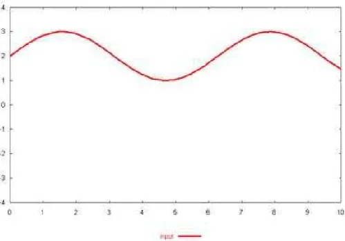
Figure 5 and Figure 6 might give a better view of this function. Figure 5 shows the input signal, Figure 6 shows the output result for the different modes: DC, AC, GND. In DC-mode giving the upper sinusoid, in AC-mode the lower one and in GND mode the output aligned to the horizontal axis.
Figure 5: the input signal
Figure 6: the output signal in DC, AC and GND mode
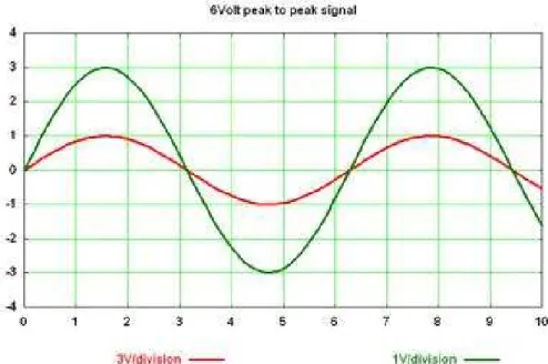
With the voltage/division knob the scale in which the input signal is presented on the
oscilloscope screen can be altered. The more volts/division, the smaller the signal will appear in the output. Figure 7 shows a sinusoid with a 3V amplitude (6Volt peak to peak), once with the voltage/division knob set on 3V per division and once on 1V per division.
The oscilloscope’s voltage/division knobs will have the following discrete values: 5, 2, 1, 0.5, 0.2, and 0.1 V/div.
Figure 7: examples of different voltage/division modes
The last setting of the vertical section is the position knob. This knob controls the signals offset in screen divisions. Both a negative and a positive offset are possible. It's used to compare the DC levels of different signals, to put both channels of the oscilloscope on the same GND-level and various other things. This is made clear in Figure 8.
Figure 8: examples of different vertical position modes
Combining the three parts of the vertical section, the following mathematical expressions can be found:
For DC mode: o(t) = (i(t) + P)/v For AC mode: o(t) = (iac(t) + P)/v
For GND mode: o(t) = P/v = constant in which:
iac(t) = alternate current part of input signal [Volt]
Idc = direct current part of input signal [Volt]
v = voltage/division [Volt/divisions]
o(t) = output from vertical section [divisions] P = position, offset [Volt]
2.3.1.2
The horizontal section (Timebase)
In the horizontal section, the following things are defined: the amount of seconds shown in one division and the reference position:
Seconds/division:
= base setting or sweep speed
This is a scale factor. Horizontally, the screen has 10 divisions. So when the setting is 1 ms, one horizontal division represents 1ms and the total screen width represents 10 x 1 ms = 10 ms (= the product of the amount of divisions (10) and the sweep speed (1ms))
Longer and shorter time intervals of the input signal can be seen on the screen by changing the seconds/division.
The display is a matrix of pixels. The hardware produces a fixed number of samples per sweep, for example 1000 samples (= buffer size). These samples should then be equally divided horizontally on the display. The horizontal scale is set by the sample rate. An example:
The sample rate is 1000 samples/s and each sweep is 1000 samples.
This means there is 1 sweep per second and because there are 10 divisions per sweep, the horizontal scale is 0.1 s/div.
To become a fluent line on the screen a good sample rate is needed. The sample rate of 10000 samples/s is set as maximum which is equal to 10 ms/div:
10000 samples = 10 sweeps = 100 div; 1s = 1000 ms;
=> 1000ms/100div = 10ms/div
The following settings are enough: 10, 20, 50 and 100 ms/div.
Sample points are digital values which can be obtained out of an analog-to-digital converter (ADC). This ADC is a part of the data acquisition hardware device. The intervals between the samples refers to the time between the sample points and will define the sample rate. An other way to set the correct timebase is altering the amount of samples by using a fixed sample rate. Reference position:
By setting the reference position you can choose the horizontal position of the trigger point. There are three discrete values: 10%, 50% and 90% of the screen. The default value is 50%.
2.3.2 In LabVIEW
As shown in Figure 4, this section contains the unbundling of the Vertical inputs, the Vertical Range.vi, the Horizontal Range.vi, the Signal Input.vi and the ACDCGNDSelector.vi. Two “Unbundle” elements split up the “Vertical A” and the “vertical B” inputs into the 4 settings for each channel: a Volt/division, a position, a boolean value that determines whether the channel is enabled or not and a slide value which determines the coupling mode (AC, DC or GND).
A description of the four subVI’s is given:
2.3.2.1
The Vertical Range.vi
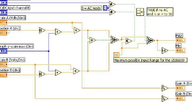
This vi gets the following inputs: The Scale (Volts/div), the Position (div) and the coupling mode of both channels and the Graph y-scale max (Div). The vi takes care of the gain calculation and the maximum/minimum value calculation (Figure 9):
Figure 9: The Vertical Range.vi
Gain calculation
The gain for each channel can be calculated by inverting the selected voltage/division value. Maximum/minimum Value Calculation
To find the maximum value, the absolute value of the position needs to be added with the Graph y-scale max. This result is an amount of divisions and must be multiplied with the scale to become a maximum in voltage. These calculations are made for both channels with an Absolute Value, an Add and a Multiply element.
The maximum in voltage of both channels now needs to be compared with each other. The highest value becomes the new maximum of the two channels. In LabVIEW this is done with a Greater and a Select element. Because the usb-6009 has a limited range, the device its maximum is +10V. This means that when the calculated value exceeds 10V, the maximum is set on 10V. This is done with another Select element.
Another exception is made when the coupling of a channel is set to AC. In that case the maximum range of the usb-6009 is used as well. This is done because there is no information
on what the maximum value visible on screen could be. This way a signal with a large offset could appear as a clipped signal on screen when the min/max values are too small.
For the minimum, the negative value of the maximum is used and can be found with a Negate element.
2.3.2.2
The Horizontal Range.vi
Figure 10: Horiz. Range.vi
In this vi, the Pretigger scans and the Sweep length (scans) are calculated out of the Time base and the Max. scan rate (Sec/div): Figure 10.
To calculate the “Sweep length (scans)”, the following formula is used:
sweep v numberOfDi s scans e MaxScanRat timebase div scans Length sweep ( )=sec/ ( )* ( / )* /
The Max scan rate is set on 24000 scans/sec determined by the USB-6009 and the Number of div/sweep is set on 20 because a buffer of 2 screens (= 20 divisions) is needed to have enough samples after the trigger. So the Sweep Length can now be calculated by multiplying these 3 values with two Multiply elements.
To calculate the “Pretrigger scans” (=amount of scans before the trigger), the following formula is used:
Pretrigger Scans = reference position (in percent of the screen) * sweeplength/2
The Sweep length needs to be divided by 2 be because the amount of Pretrigger scans is for 1 screen. This can be calculated with one Multiply and one Divide element.
2.3.2.3
The Signal Input.vi
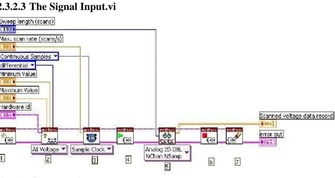
Figure 11: Signal Input vi
In Figure 11 there is a picture of the Signal Input.vi in LabVIEW. It needs the following inputs: the sweep length, the Max. scan rate (scans/s), the maximum and the minimum value (calculated in the Vertical Range.vi) and the Hardware id. The hardware id is on most computers the default id (=Dev1/ai0,Dev1/) for the USB-6009. Generally this is the appropriate setting and it only needs to be changed in rare cases.
The 7 numbered blocks in Figure 11 acquire the data out of the USB-6009 A short overview of those blocks:
1. An empty task is created.
2. An analog input voltage channel is created. The hardware id is selected, and the gain in the programmable gain amplifier is set trough the maximum and minimum value. Also the measuring mode is set (differential).
3. Here the scan rate is set on the highest possible scan rate. The sample mode is defined to be continuous.
4. The start VI: The data acquisition starts here.
5. The “number of samples per channel” is set as the sweep length (amount of scans) and the data output returns the Scanned voltage data record.
6. Stop the analog input task.
7. Call the clear Task VI to clear the Task.
The output of this VI now gives the Pretrigger scans, the Sweep length (in amount of scans), one array with two rows of Sampled Voltage Data and eventually error messages when an error occurred.
2.3.2.4
The ACDCGNDSelector.vi
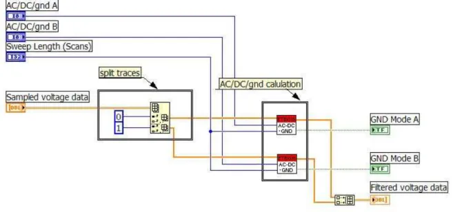
This vi needs the following inputs: the AC/DC/gnd setting of channel A and B, the sweep length (Scans) and the Horizontally adjusted voltage data (see Figure 12).
Figure 12: The ACDCGNDSelector.vi
First of all, the 2-dimensional array is split into two 1-dimentional arrays to do the appropriate calculations according to the vertical settings for each channel. Each of the resulting arrays contains the data of one channel. This splitting is done with the following function: Index Array. This element needs a n-dimension array (the horizontally adjusted voltage data) and one or more indexes as input and it returns the element or sub-array at the given index (0 and 1).
After this, there is taken care of the AC/DC/gnd calculation with an AC-DC-GND.vi for each channel. This vi calculates the “Horizontally adjusted voltage data” and a “GND Mode” boolean for each channel, according to the AC/DC/gnd setting.
The following inputs are needed: the Sampled adjusted voltage data of the appropriate channel, the AC/DC/gnd setting of that channel and the Sweep Length (Scans)
There has to be a distinction between the 3 cases: In LabVIEW this is done with a case structure. In such a case structure, the value wired to the selector terminal (at the selection mark sign) determines which case to execute:
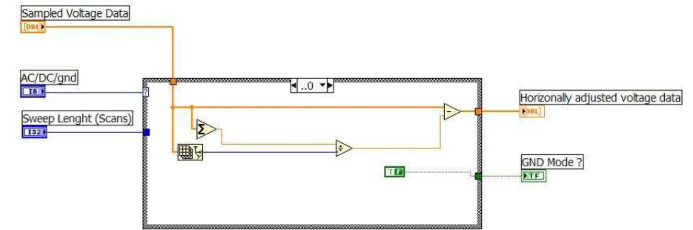
- In case of AC (Figure 13):
In this case, the sum of data values out of the array is made and this has to be divided by the size of the array to get the average. For each of these 3 calculations, there exists a function in LabVIEW: Add Array Elements, Array size and Divide.
The distraction of the original values with this average will give the Horizontally adjusted voltage data as output. This is done with a distract element which distracts the calculated value of all elements of the array.
Also, the GND mode boolean is set on false. This boolean will be used later on in the program.
Figure 13: case AC
- In case of DC (Figure 14):
In this case, the original data has to be shown on the screen, so the Sampled voltage data is directly connected to the Horizontally adjusted voltage data output. The GND mode boolean is again set on false
Figure 14: case DC
- In case of gnd (Figure 15):
In case of gnd mode, all the data values in the array must become zero. The Initialize Array function makes a brand new array full of zeros. This function needs an element and a size as input and creates an n-dimensional array in which every element is initialized to the value of that element. The size of the new array is determined by the Sweep Length calculated in the Horizontal Range vi. Of course the GND boolean is now set on true.
2.4 Trace extraction
This section mainly consists out of calculations and checks that have something to do with the triggering. A theoretical background of the Trigger section is given before explaining the implementation in LabVIEW:
2.4.1 Theoretical Background
The trigger section is used to control the starting point of the sweep on the display. Always triggering on the same point is necessary to become an apparent fixed image of the input signal.
The trigger level control makes it possible to select the voltage at which the waveform starts, the slope control selects whether the waveform starts at a positive or at a negative slope. When the input waveform gives a slope and level match at the reference position, as set on the trigger and horizontal control panel, a pulse is sent to the horizontal circuit section to start the sweep. Periodic input signals will start the sweeps at the same point, which will give a
stationary signal on the output screen.
There are three different trigger modes: Normal triggering, auto triggering and auto-level triggering.
Normal triggering is the most basic of all triggering methods. First the trigger level must be selected. If the trigger conditions are not reached, there wont be a sweep.
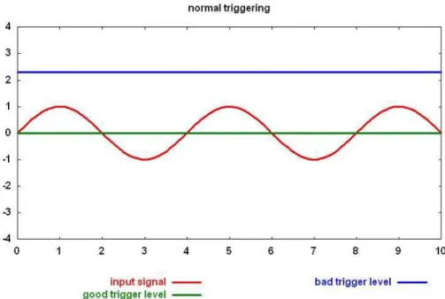
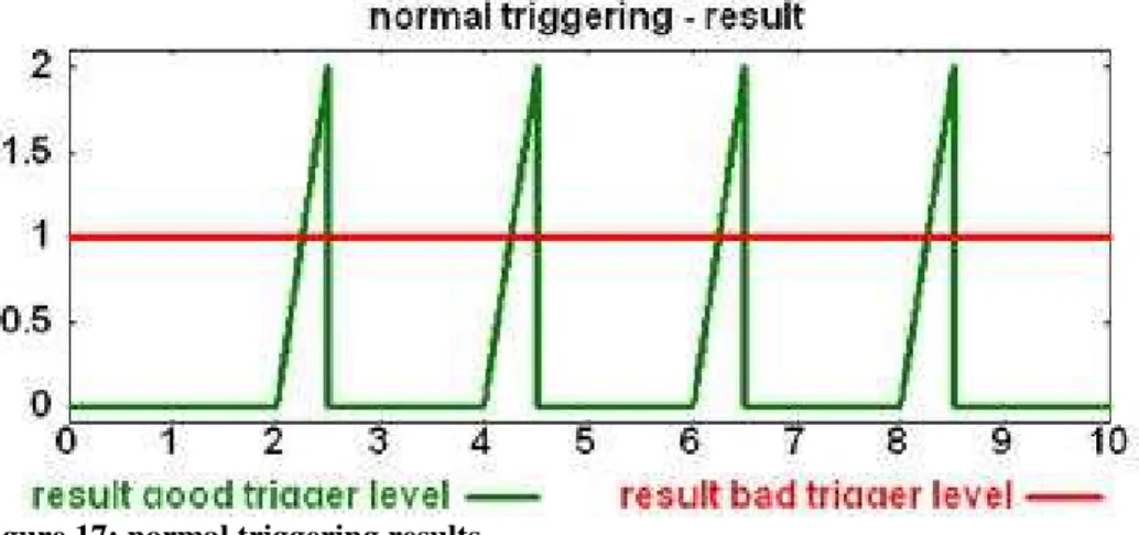
Figure 16 and Figure 17 can clarify this. In Figure 16 the input signal and two trigger levels are shown. One of the trigger levels is clearly not crossed by the input signal and the other one crosses it periodically. The results of the trigger level can be seen in Figure 17. For better viewing; both trigger signals are on a different base level. The bad trigger level doesn't cross the signal and will result in a non changing trigger signal. It provides no trigger pulses and thus no sweep. The good trigger level does cross the input signal. In Figure 16 there is triggered on the negative slope: a trigger pulse will be generated on the trigger signal, every time the input signal is on a negative slope and crosses the trigger level.
Figure 17: normal triggering results
Auto-level triggering is very similar to normal triggering. In this trigger method, the
oscilloscope will first fire a random sweep, measuring the maximum and minimum level of the input signal. The trigger level will then be put in the middle between those boundaries, resulting in a guaranteed trigger if the signal is recurrent.
The difference between level and normal triggering thus lies in the fact that the auto-level trigger takes control over the trigger auto-level selection.
When using auto triggering, the trigger circuits in the scope waits for the input signal to reach the trigger conditions. If the input signal does not reach the trigger point within a
pre-specified time interval (timeout), the scope will automatically generate the trigger pulse causing a sweep to start.
2.4.2 In LabVIEW (Extract Traces.vi)
As shown in Figure 4 , this sections only contains the “Extract Traces.vi” (Figure 18).
Figure 18: Extract Traces.vi
This VI starts with separating the Sampled voltage data of channel A and B from each other with an “Index Array” element. The source boolean which comes out of the Trigger cluster must select which channel must be used for triggering. The boolean is true when channel A is the trigger channel and false when channel B is the trigger channel. The selection of the correct trigger channel is made with a “Select” element.
The actual sweep length in traces is the half of the sweep length in scans that is given as input. The difference is that the actual sweep length is for one screen while the sweep length in scans is for 2 screens.
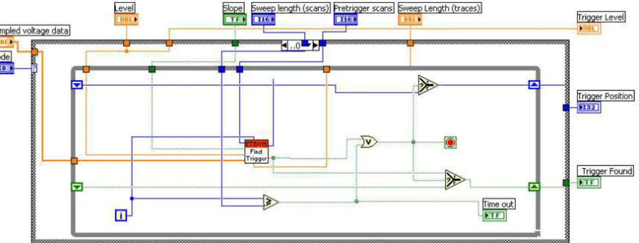
The trigger subVI calculates the trigger position and returns a boolean that determines whether a trigger is found or not. This vi contains one big case structure, controlled by the way of triggering: normal (case 0), auto (case 1) or autolevel (case 2) triggering. In every case there is a Find Trigger.vi (Figure 19) used in a while loop to find a usable trigger. This vi works as follows:
Figure 19: Find Trigger.vi
A way to search the trigger point is by checking if the trigger level is passed between two successive values: the “Iterations of the while loop” input and a decrement of this input selects 2 such successive values out the “Sampled voltage data” by using an “index array” element. Those two values (sample A and B in Figure 20) are compared with the trigger level and if one of them is higher and the other one is lower than the trigger level, the trigger level is passed. This is implemented with 2 comparing elements (an “Greater Or Equal” and an “Equal” element) of which the outputs are connected to an “Exclusive Or” element.
If, for example, both results from the comparison are “TRUE”, then both signals are below the trigger level, and the XOR port will return a “FALSE”.
Figure 20: Checking for trigger
Next thing to do is check for the correct slope. All that has to be done for this is comparing the current value with a value of two places before. This last value is also returned by the
“Index Array” by giving as index input the “Iteration of the while loop” minus two (= 2 times a decrement). There is a correct slope when this comparison is in order to the slope boolean: so there is a combination of a “Less?” element and a “Equal?” element needed.
When the trigger level has been passed and the slope is correct, a trigger has been found. The next step is checking if the trigger is in range. To do this the amount of pretrigger scans are subtracted from the previously found trigger location: this gives the start location from the scans that will be used to fill up the screen. After that, two comparison elements are used to check whether there are enough samples available to fill up the whole screen.
If the result of these 4 checks are true (the and port of the 4 result becomes true) a usable trigger has been found. The position of this trigger is passed on, together with a “TRUE” Boolean to indicate that a correct trigger has been found.
After understanding this subVI, the 3 cases can be explained: Normal triggering (case 0)
In this case (see Figure 21), a while loop is used to try to find a successive trigger with the Find trigger.vi. This loop will continue until a successive trigger is found or until the amount of iterations gets bigger then the amount of scans (sweep length) which means there is a timeout. This is implemented with a “Greater or Equal?” element between the Sweep length and the amount of iteration which leads to a “Time out” output. This output in combination with the “Trigger Found” output of the Find Trigger.vi are connected to an OR-port which returns the boolean of the while loop condition. When the condition to stop the loop is reached, the “Trigger Found” and the “Trigger Position” outputs must be changed to the outputs of the Find Trigger.vi and otherwise they stay the same as in the previous iteration. This is implemented with 2 “Select” elements. The “Trigger Level” can directly be connected to its input because when there is no trigger found, this level doesn’t matter.
Figure 21: Normal triggering
Auto triggering (case 1)
The only difference with this trigger mode is that it triggers after a certain amount of
iterations instead of stopping the search for a trigger when the number of iterations gets bigger then the sweep length (see Figure 22). When no trigger is found after 52% of the sweep length the while loop must stop and there must be a triggering on the last used trigger position: this means that the “Trigger Position” changes to the output of the Find Trigger.vi which is done with a “Select” element. 52% of the sweep length is used as limit because then there are still enough scans left in the buffer. This in consideration with a minimum Reference position of
10%. Before this auto triggering takes place, normal trigger conditions will be searched using the same method as in normal triggering.
After the while loop has ended the level from the trigger position is fetched from the
“Sampled voltage data” with an “index array” element. In case of a timeout this new trigger level will be used as trigger level, in case of a normal trigger the preset trigger level will be used. This selection is made with a “Select” element. Because there will always be a triggering in this mode, the “Trigger Found” output can be set on true.
Figure 22: auto trigger
Autolevel triggering (case 2)
Autolevel triggering starts by calculating a new trigger level (see Figure 23). The “array max & min” function gives the maximal and minimal value of the data array from the selected channel. The sum of those two values divided by two gives the new trigger level. The actual triggering goes in the same way as the normal triggering. The only difference is that there will definitely be a trigger in this mode, so no “time out” precautions are necessary.
Figure 23: Autolevel Triggering
If a trigger has been found (the “Trigger Found” boolean out of the Trigger.vi is true), the new data-arrays can be created with a subset array starting from the trigger position (Figure 24). The size of these new arrays is determined by the Sweep length (traces for one screen). Then both arrays are bundled and sent to the “map to graph” subVI.
Figure 24: New Data-Array (trigger)
If there is no trigger found, all data in the new arrays will be set to “zero” (Figure 25). This array will also be used in case of ground mode coupling to present the ground-line on screen.
Figure 25: New Data-Array (no trigger)
Those two cases are implemented with a case structure.
At the and of the Extract Traces.vi, the “Cursor Trigger Level” output is determined: it is a cluster of the trigger level with the boolean that determines the source of the trigger (in case of true, channel A is the source of the trigger and in the other case channel B). This cluster is needed in the Map to Graph.vi.
2.5 Display of the traces
As last part there is the “Display of the traces” section that needs to take care of the output. First of all this means that the vertical adjustments have to take place so the plots appear on the screen in the right proportions and on the right position. This is done in the Map To Graph.vi which will give the traces to put on the Waveform Graph and the Trigger Level as output. Secondly, a Waveform Graph block is used to configure the Waveform Graph:
2.5.1 The Map to Graph.vi
After splitting up the voltage data, both channels arrays are formatted in the appropriate way. The following formula is used to do this: “input∗gain+ position”. Here the input is the array of data values. In LabVIEW this formula can be created using a Multiply and an Add element (see Figure 26). After this, the data values of both the channels are collected again with a ‘build array’ component. The “traces” output is ready to be submitted for the waveform graph.
The trigger section of this vi starts by selecting the correct gain and position values to adjust the trigger level, so it can be positioned correctly on the screen. This is done with a case structure: if the boolean of the cursor trigger is true, the values of channel A must be taken and in case of false the values of channel B. After this, the trigger level also is vertically adjusted, using the same formula as before. This adjusted trigger level will be displayed on the screen later on.
Figure 26: Map to Graph.vi
2.5.2 Configuration of the Waveform Graph
Completely on the right (Figure 4) there is a column shown, called Waveform Graph property node. This block places the different cursors on the graphical output: the trigger level, the position of channel A and B, and the reference position. The ActCrsr is used to get and set the active cursors and set properties and methods on that cursor. The Cursor.PosX/Y is the X/Y coordinate of the cursor: The Y coordinate of the trigger level cursor is determined in the Map to Graph.vi, the Y-coordinates for the channel A and B cursors come out of the “Vertical A”
and “Vertical B” clusters, and the X-coordinate of the reference position is set on the amount of pretrigger scans as returned by the Horizontal Range.vi.
Also the plots are controlled in this property note: ActPlot shows which plot is active. In this case there are 2 plots: one plot for each channel. The Plot.visible? makes the plot visible when it gets a true boolean as input. A plot must only be visible when the ON/OFF button is in position ON and if the trigger is found or the channel is in GND mode. This is determined with an OR in combination with an AND element.
Every cursor and every plot also gets a number assigned that is used as index for that cursor/plot.
The Xscale.Maximum is the maximum value of Scale which is determined by the Sweep Length and the XScale.Increment is the increment value of the scale which is 1/10th of the Maximum value of Scale to become 10 divisions.
The “Hide Grid” boolean determines whether the grid has to be visible or not: in case of true the X- and Ycolor are set in a color (26112 and 13056 stands for 2 kinds of green), in the other case they are set black (0 stands for black) which is implemented with a “Select”
element. A cluster of two colors is needed as input to set the X/Y color: The first one is for the major color and the second one for the minor color.
2.6 Performance
The performance of the application is mainly dependant on the USB-6009. This device has a rather small maximum scan rate. The performance of the application is thus satisfactory. On relatively slow computer hardware (Pentium II 400 MHz, 256 MB SDRAM, 100MHz FSB) the oscilloscope reacts prompt. Only when changing the input signals very quickly the oscilloscope needs a little bit more time to recalculate the signal. This is due to the slow USB protocol and because of the needed calculations. The response time is generally quite short and is most of the times negligible.
There is only one performance problem: an error -200361 dialog (Figure 27) sometimes pops up in the following cases:
• when there are a lot of programs in the computer's memory • by using a lot of debug features
• or very rare, while only working with the oscilloscope
National Instruments website states the following about the problem:
Solution: The behavior you are experiencing is a result of a combination of factors.
1. The 6008/9 has a relatively small onboard FIFO. 2. NI-DAQmx Base is a driver written at the user level.
3. Communication with the device is message based over USB which is inherently slower than equivalent communication over PCI.
Since NI-DAQmx Base is written in LabVIEW, it has user level priority and CPU allocation. If the operating system is busy with other user level operations, NI-DAQmx Base can get starved of resources so that it cannot request data from the USB device fast enough. Since the USB-6008/9 has a relatively small onboard FIFO, it does not take long for the FIFO to overflow if you are acquiring at a high rate. Unfortunately, the operations such as opening other programs, minimizing/maximizing windows are very CPU intensive, especially with Windows OS. Therefore, when you perform these operations, NI-DAQmx Base cannot retrieve data from the device, the FIFO overflows, and you get the -200361 error.
Investigation about the USB protocol problem is easy: The program is tested over USB1.1 (up to 12mbyte/s) and USB2.0 (up to 480 mbyte/s). There was no difference in performance. The conclusion is thus that the error always comes from a combination of the relatively small onboard FIFO and the driver being written at user level. Testing on several computers confirmed this. In the end it seems that this error is impossible to solve in the program code; it's one of the limitations of the USB6009 device. One possible solution is to filter out the error message because it's actually only a warning and the program continues working after pushing the ok button.
3 A more advanced oscilloscope using a high speed
digitizer
3.1 Introduction
This section describes a more advanced scope which uses a high speed digitizer, the NI5112, to acquire the data, instead of getting data from a simple DAQ-board. A high speed digitizer is a piece of equipment that reads in a signal and transforms it into digital data. Other
functions that distinguish the digitizer from a normal DAQ board, are that it can trigger and perform a variety of measurements on the acquired signal.
3.1.1 Advanced Oscilloscope
The advanced oscilloscope distinguishes itself from the basic oscilloscope in this way that it has a bigger variety of functions. Not only is it capable of everything the basic scope can do, it also can perform measurements on the signal directly in the NI5112.
Another difference is that you have the choice for the trigger: it can be done in the hardware of the NI5112 or it can be done by software, the same way as in the basic oscilloscope.
3.1.2 Remote Lab
A remote lab or distant lab is a laboratory that emulates a traditional laboratory. The hardware and electrical components are wired in a circuit by the use of a robot. This happens on the server side. The robot is controlled by a client somewhere else. The internet is used as the communication infrastructure between the client and the server applications.
A remote lab has some special requirements:
All settings and data have to be sent from the client to the server flawlessly. In order to achieve this goal, the data has to be sent in a predefined way. Therefore strings are used for the communication protocol.
The client sends one string which contains all settings to configure the oscilloscope in the appropriate way. The server responds with a string containing all actually used settings, the received measurements and signal data. The protocol describing these string can be found in Appendix C/D.
Because these special needs of the remote lab, the advanced oscilloscope is split up in two main vi's: The OscSetup and the OscRead.vi. The OscSetup.vi handles the first string, created by the remote front-panel. In this way the settings from the client are passed to the
oscilloscope. The second string returns the actual measurements (based on the settings out of the first string) back to the client: this is done in the OscRead.vi. This vi is executed by a second string coming from the client. This string is no more than a “send data” request. A better description is provided later on in the ‘Notes for client module implementation’. The oscilloscope also needs the resource name and an error in as input. Trough the whole program the error in will always be passed on to the next subvi and will be updated when an error occurs. The final outputs are an error out and a response string. The error out contains all the occurred errors if any and the response string will contain the results of the performed measurements.
3.1.3 Data acquisition using the NI-5112
The acquisition
The NI 5112 acquisition system controls the way samples are acquired and stored. Two sampling methods are available: real-time sampling and random interleaved sampling (RIS). Real-time sampling allows you to acquire data at a rate of 100MS/n, where n is a number from 1 to 100e+6. In RIS mode, you can sample at rates of 100MS/s*n, where n is a number from 2 to 25
During the acquisition, samples are stored in a circular buffer that is continually rewritten until a trigger is received. After the trigger is received, the NI 5112 continues to acquire posttrigger samples when a posttrigger sample count is specified. The acquired samples are placed into onboard memory. The number of posttrigger or pretrigger samples is limited only by the amount of onboard memory.
The NI 5112 PGA offers a variable input range per channel, from ±0.025 V to ±25 V. The ADC is only 8 bits. To get accurate measurements it is very important to set the PGA to the preferred range.
The triggering
The analog trigger on the NI 5112 operates by comparing the current analog input to an onboard threshold voltage. This threshold voltage, the trigger value, can be set to any voltage within the current input range. A hysteresis value associated with the trigger is used to create a trigger window the signal must pass through before the trigger is accepted. (see Figure 28)
Figure 28: Trigger with hysteresis
The NI5112 features
The supported features can be found in the table in Appendix B.
One thing that has to be noticed is that the NI 5112 only support AC and DC coupling so the GND coupling must be implemented in software.
3.2 Digitizer setup (the OscSetup.vi)
The first two things that happen in this vi is the initialization of the oscilloscope driver in the niScope Initialize.vi and splitting up the Oscilloscope Setting Information String (=Data In) with the Strip_String.vi to become the settings. The boolean of true that is one of the inputs of the niScope Initialize.vi is meant to reset the instrument during the initialization procedure.
The instrument handle output identifies a particular instrument session so it needs to be passed on to every subvi. The Strip_String.vi will give the settings, a boolean and the remaining string as output. The boolean determines whether it is Autoscale mode or Normal mode and a case structure will send the necessary inputs to the correct vi (so to the
Autoscale.vi or to the NormalSettings.vi) to do the setup according to the mode. After this, the Oscilloscope Driver can be initiated with the niScope initiate Acquisition.vi which will return an error out and the instrument handle which must be bundled with the settings and remaining string to become the output cluster that is needed for the Data Fetch. This all is shown in Figure 29.
Figure 29: OscSetup.vi (autoscale)
3.2.1 Strip_string.vi
The string that enters this vi contains the settings including a boolean to distinguish the Normal mode from the Autoscale mode. The first thing that has to be done is to strip of this boolean with a Scan from String element. The different settings can now be determined out of the remaining string. These settings includes the horizontal configuration, the channel (2 times), the trigger and the measurements (3 times) -settings.
The horizontal configuration settings
This is the first part that has to be scanned out of the remaining string and it contains the minimum sample rate (a double), the reference position (a double) and the record length (an integer). The stripping of these 3 values can, again, be done with a Scan From String element. By bundling these three values, the horizontal configuration setting is determined.
The channel settings (two times)
These settings include a boolean that defines whether the channel is enabled or not. If the channel is enabled, it also includes the vertical coupling (Enum), the vertical range (double), the vertical offset (double) and the probe attenuation (double) settings. So first the boolean needs to be scanned out. After this, a case structure will scan out the other 4 values in case of a true boolean. In case of a false boolean, the 4 other values are set to a fixed value. These 5 values are bundled together to become the settings of one channel.
The trigger settings
These settings include the source (Enum), the slope (Enum), the coupling (Enum), the level (double), the holdoff (double), the delay (double), the mode (double) and the timeout (double) –settings. The scanning of these values is analogue as in the previous settings.
The measurement settings (three times)
All this results in the following outputs: -Autoscale/Normal
-Remaining String
-Settings: Horizontal Conf.: Min. Sample rate (a cluster of) Reference position Record Length Channel A: Enable Vertical coupling Vertical range Vertical offset Probe attenuation Channel B: Enable Vertical coupling Vertical range Vertical offset Probe attenuation Trigger: Source Slope Coupling Level Holdoff Delay Mode Timeout
Measurements: Measurement 1: Channel Selection Measurement 2: Channel
Selection Measurement 3: Channel
Selection The result of all this is shown in Figure 30.
Figure 30: The Strip String vi
3.2.2 In case of Autoscale mode: niScope Auto Setup.vi
If autoscale is used, the oscilloscope makes all settings according to the signal. This function is created by National Instruments: the niScope Auto Setup.vi. This means that in this case the settings doesn’t need to be changed and the adjusted instrument handle and the error out are given by the niScope Auto Setup.vi: Figure 31.
Figure 31: Autoscale Mode
3.2.3 In case of Normal mode: NormalSettings.vi
The NormalSettings.vi will return the adjusted instrument handle out and the adjusted trigger level started from the instrument handle in (out of the niScope Initialize.vi) and the Settings (out of the Strip_String.vi). A bundle by name element will replace the trigger level in the cluster of settings with the adjusted trigger level in auto-level triggering mode (see Figure 32). This is only for later developing purposes because the actual used trigger level is returned by the driver (see later).
Figure 32: Normal Mode
The NormalSettings.vi contains four parts that are connected behind each other by passing on the errors and the instrument handle: Figure 33.
In the first part the “niScope Configure Acquisition.vi” is used to set the scope in Normal acquisition mode. In the second part, the “niScope Configure Horizontal Timing.vi” takes care of the configuration of the horizontal settings. This vi needs except for the instrument handle and the error input also the minimum sample rate, the Reference position and the Record length as input: unbundling the “Horizontal Conf. input” gives these values. The last two parts consists out of the “Vertical settings.vi” and the Trigger.vi.
Figure 33: The Normal.vi
In the Vertical settings subVI (see Figure 34), the Channel A and Channel B settings are used as input. The “Vertical range” outputs are created for each channel out of the channel A en B setting clusters. All the settings of Channel A and Channel B each go to a “niScope Configure Vertical.vi”. When a channel is GND coupled, it’s necessary to change this coupling mode because it is not supported by the NI 5112. Later on in the program the GND coupling will be implemented in software. In this case, a change from GND to DC-coupling is used: this is done with a case structure in the checkforground.vi that can be seen in Figure 35.
Except for these channel settings, the “niScope Configure Vertical.vi” also needs the instrument handle, the error in and the channel name as input (0 for channel A and 1 for channel B). Coupling those 2 “niScope Configure Vertical.vi’s” behind each other will give the adjusted instrument handle and the error out as output. Both channels are always enabled so its possible to trigger on a disabled channel and to perform measurements between both channels: for example to determine the phase delay.
Figure 34: The vertical Settings.vi
Figure 35: The checkforground.vi
The Trigger subVI needs the Trigger settings and the Vertical range of Channel A and B as input. First the appropriate trigger source is selected. A distinction is made between triggering on channel ½, Immediate triggering and external triggering by using a case structure.
In case of Immediate triggering
When an acquisition is initiated, the digitizer waits for the start trigger. In this case the digitizer triggers immediately when the acquisition is started. This setting is done in the “niScope Configure Trigger Immediate.vi”. This vi only needs the instrument handle and the error in as input. With immediate triggering the trigger level is unused so it is set on a
constant to avoid errors: Figure 36.
Figure 36: Immediate triggering
In case of External triggering
In this case the triggering is configured the same way as is the case of immediate triggering because external triggering is not necessary in a remotely operated laboratory. Thereby it is not implemented in the current version of this program.
In case of Channel 1 or Channel 2 as trigger source
Because all of the niScope vi’s need a string of the channels List as input instead of a double, the source of the trigger is first converted with a Number to Decimal element. Depending on the trigger mode (Auto/Normal or Autolevel), the trigger level is determined in a case structure:
-In case of Autolevel mode (Figure 37):
Figure 37: Autolevel mode
First of all a niScope Configure Trigger Immediate.vi is used so there will be an immediate triggering. Secondly the niScope Initiate Acquisition.vi makes the oscilloscope leave his idle state and initiates a waveform acquisition. The Check Status.vi (see Figure 38) executes a while loop until the acquisition status is equal to 1 which means the driver is now completely ready to do measurements. This happens in a No error case structure because otherwise the program gets stuck because the driver never gets ready as the oscilloscope is not configured properly.
Figure 38: Check Status.vi
After this, there are two niScope Fetch Measurements.vi’s used to calculate the trigger level: The scalar measurement of the first vi is equal to 6 which stand for Voltage Max so this vi will give the maximum voltage as output. The second vi will search for the minimum voltage (scalar measurement = 7). The trigger level is now the average of the minimum and the maximum voltage (the summation divided by 2). At last the niScope Abort.vi aborts the acquisition and makes the program exit the measuring mode so the oscilloscope settings can be altered again.
-In case of Auto or Normal trigger mode (Figure 39):
In this case the trigger level stays the same as in the trigger settings.
Figure 39: Auto or Normal trigger mode
To become the final trigger level, there needs to be a check whether this (calculated) trigger level is within the Vertical range of the channel of the trigger source. If the trigger level is out of this range, a fatal error will occur. Therefore the following steps are made: the trigger source is checked and the vertical range of that channel is taken: this is done with an “Equal?” and a select element. When half of this Vertical range (by using a dividing element) is higher then the trigger level, the trigger level is out of range and the final trigger level becomes the maximum possible trigger level for this vertical range. If the trigger level is in range, the correct level is used. This is done with a comparing and a select element.
After this, the niScope Configure Trigger Edge.vi configures the driver for edge triggering with the appropriate settings.
3.3 Data fetch (OscRead.vi)
The actual acquisitions starts in this vi. The DAQ will fetch the data and convert it into strings to send back to the client. All the settings from the first string are passed trough from the OscSetup.vi. As the driver is already configured in the OscSetup.vi, the only thing that needs to be done here is performing the measurements, error handling and building the response string.
Figure 40: The OscRead.vi
The Channel list, consisting out of 1 constant string (0,1), is used to enable both channels for the measurements. The reasons for this are already mentioned before. Some settings coming from the OscSetup.vi trough the output cluster are clustered and are passed to the appropriate vi’s. Like in the OscSetup.vi the instrument handle and the errors are always passed trough the different blocks in the block diagram.
3.3.1 niScope Multi Fetch Binary 8.vi
The scaled voltage data is fetched here in consideration of all settings made before. This vi returns the ”wfm” and the “wfm info” as output. The waveform (wfm) is an array of clusters, each containing the “initial x value”, the “x increment” and a waveform array per channel. The waveform info (wfm info) is an array of clusters which contains all the timing and scaling information for each waveform (actualSamples, absoluteInitialX, relativeInitialX, xIncrement, gain and offset).
3.3.2 CheckError.vi
The task of this vi is to check whether the Multi Fetch Binary 8.vi was able to perform his task correctly. The vi checks wether the “BFFA2003”-error occurred, which is the
“niscope_error_max_time_exceeded” error. It indicates a trigger timeout.
First step is to unbundle the error cluster and check if there actually is an error (this is determined with the boolean out of the cluster). The two cases are split up with a case structure:
In case of false:
If there is no error, the “error in” just gets connected to the “error out” and the “Time out” remains false.
In case of true:
If there is an error, there are two possibilities: the error is equal to the “BFFA2003” error or it is not. This is checked with an Equal element so the two cases can again be split up with a case structure. The result of the Equal element also determines the Time out boolean.
In case of false: the error is not equal to the “BFFA2003” error
In this case there is another error which must be connected to the “error out”.
In case of true: the error is the “BFFA2003” error
Because the Time out became already true, the error gets reset.
3.3.3 The Check Trigger vi
Figure 42: the Check Trigger.vi (case true, Auto Mode)
Depending whether the timeout occurred in the “Multi Fetch Binary 8.vi”, an appropriate case is selected.
In case of false the time out didn’t occur so the data can be passed on directly to the Scan to String.vi.
In case of true the Timeout occurred. The triggering mode is changed into immediate
triggering. First the acquisition needs to be aborted (niScope Abort.vi) then the oscilloscope is configured for immediate triggering (niScope Configure Trigger Immediate.vi) and finally a waveform acquisition can be initiated again (niScope Initiate Aqcuisition.vi): see Figure 42. Again the Check Status.vi is used to check whether the oscilloscope is ready to perform measurements (see earlier).
After this a distinction between Normal/Auto Level and Auto is made:
In case of Auto Mode
In this case the oscilloscope has to trigger immediately so the niScope Multi Fetch Binary.vi can just start to Fetch data. This vi will return the adjusted “wfm info”, “wfm”, instrument handle and error out as output.
In case of Normal/Auto Level
In this case, it was not possible to trigger with the configured settings. No data is fetched and in the response string there won’t be any waveform data included. Normally in Autolevel, there won’t be a timeout but a case for this is mandatory in LabVIEW.
3.3.4 The measurements vi
The task of this vi is to perform measurements on the data channels.
Figure 43: measurements.vi
The measurements cluster contains three pairs of values (one pair per measurement) determines which measurements are requested on which channel.
First the instrument handle and the error in are given as input to a Property Node element which gets and/or sets properties of the reference. In this case channel B is used as reference to make for example phase measurements on channel A and vice versa. This element will return the adjusted instrument handle and the errors.
For every measurement that needs to be executed, a measurement request and a channel (both from the “measurements cluster” input) must be linked to the “Execute Measurement” subVI.
Figure 44: Execute Measurements subVI
In case the Error In contains an error, the instrument handle and error signal will be directly connected to the output. The result will be set to “0,0”. If there’s no error, the first step in the “executemeasurements” subVI is checking if the channel on which the measurement must be done is enabled. This is done with a case structure in the “Check_Channel” subVI: it will return a true boolean if the requested channel is enabled. A Measurement Selection of 4000 means that no measurement is requested. So only when the channel is enabled and the
Measurement Selection is not equal to 4000, a measurement will be performed. This check is done with an Equal, a NOT and an AND logical port. The result of the AND-port is connected to the selector terminal of a case structure:
In case of false: No need for measuring
The instrument handle in and the error in are directly connected to the instrument handle out and the error out. The result must be set on 0,0 as specified in the protocol.
In case of true: Measuring is necessary
For doing the measurement, the niScope Fetch Measurement.vi is used. The channel needs to be in a string form so a Number to Decimal String element is used to make the correct
conversion. The timeout is set on zero to tell the NI-scope to fetch whatever is currently available.
The results of the three Execute Measurements can now be clustered together for submitting them to the Scan to String.vi.
3.3.5 The scan to String vi
Figure 45: Scan to String vi
Appendix D). This string must contain the following values: -Horizontal: the actual sample rate and the actual record length.
-Channel (2 times): the probe attenuation, the vertical range, the vertical offset, the gain and the waveform (which is an array of bytes).
-Measurements (3 times)
-Trigger: the received boolean and the level.
The actually used horizontal values are fetched with the “niScope Sample Rate.vi” and the “niScope Actual Record Length.vi”. If both channels are disabled, the actual record length is set to zero. The NAND port behind the “channels cluster” takes care of that. After that they are put into a string with a Format Into String element.
Now the vertical settings are added to the string. The probe attenuation and the vertical range are fetched from the “niScope Query Vertical.vi”, the offset and gain from the “wfm info”. The “Channel on/off” subVI (Figure 46) then checks if the channel is enabled. If this is the case it will execute the “Array2string.vi” which will convert the data array into a string. If it is disabled a new array (size equal to the actual record length) with only “zero” values will be created instead of the actual data.
Figure 46: Channel ON/OFF vi
Figure 47: Array2String.vi
The array to string conversion is executed in a while loop. For every iteration until the actual record length is reached, an element is fetched from the array and added to a string using a format into string element. This string is passed on to the next iteration using a shift register. Once the actual record length is reached the complete string can be sent to the output. After adding this string the results (doubles) from the three measurements are added to the string, followed by the information on the trigger which contains one Boolean (trigger found or not) and one double containing the trigger level. This last value is fetched out of the “niScope Query Trigger Edge.vi”.
3.3.6 The niScope Abort and the niScope Close vi
After making all the necessary measurement to create the needed Output string for this “OscRead” vi, the acquisition needs to be aborted and the session needs to be closed to be ready for a next cycle. This is done with the niScope Abort and the niScope Close.vi. The
“niScope Abort” vi gets the “instrument handle” and the “error in” inputs from the Scan to string vi and the outputs of this “niScope Abort” vi are the inputs of the “niScope Close” vi.
3.4 Notes for client module implementation
As already stated before this oscilloscope is structured in two blocks. The reason for this is the need to use the oscilloscope remotly controlled. The oscilloscope is completely operated by a normal text string. The oscilloscope works with two setup strings and one response string. A first string is used to configure the oscilloscope. This string executes the OSCsetup virtual instrument. This VI calculates the needed values (for example the trigger level in autolevel triggering mode) and passes them to the oscilloscope. This VI doesn't return anything to the client.
The second step the client needs to do is asking the data by sending another string. This will execute the OSCread VI. This VI will perform all the requested measurements and return the available data in a response string to the client.
The client module should take care of sending the two strings not too fast after each other because the OSCsetup needs time to execute. Also for some settings the client module has to take care that their values are not going out of bounds as this will result in an error not reported in the output string.
Another point the client should take care of is the enabling/disabling of channels. When both channels are disabled, the oscilloscope won't return any data for any channel. However when only one channel is disabled, the oscilloscope will send an array of zero's instead of that channel's data. The client should recognize the on/off state in it's own control panel and take care of this by itself.
For the appropriate string settings and response (the protocol) we refer to the Distance Laboratory, Protocol Specification version 3.0 available at the Blekinge Institute of Technology. The oscilloscope part of this is found in Appendix C and
Appendix D.
For the possible measurements and the boundaries that should be respected in the setup string; we refer to the NI 5112 digitizer manual available at the website of National Instruments.
3.5 Test environment
To check the proper functioning of the OSCsetup and the OSCread a test environment has been created. It replaces the user interface that will be used to control the more advanced oscilloscope once it is implemented in the remote lab.
The test environment consists out of three sections: a “Setup section”, a “Read section”, and a “Graphical output”. The purpose of the “Setup section” is to send all necessary parameters in a string to the OSCsetup.vi. The “Read section” will transform the string received from the OSCread back to separated and useful values. The “Graphical output” will give, much like a real oscilloscope, a quick image of the acquired signal.
During the tests, the oscilloscop reads in data from a function generator with known settings.
3.5.1 Setup Section
The front panel of this part of the test environment looks like the control panel of a normal oscilloscope (see Figure 48). In case of “autoscale” the OSCsetup will ignore all parameters that you define here, so for testing purposes it should be placed in the “OFF” position. The “remaining string” element is solely for testing purposes, all data in that controller should be ignored and passed on by both the OSCsetup and the OSCread. The other controls will provide parameters according to the “oscilloscope request protocol” (see