1
CHAPTER
4
CHAPTER
ARE GLOBAL IMBALANCES AT A TURNING POINT?
Global current account (“flow”) imbalances have narrowed significantly since their peak in 2006, and their configura-tion has changed markedly in the process. The imbalances that used to be the main concern—the large deficit in the United States and surpluses in China and Japan—have more than halved. But some surpluses, especially those in some European economies and oil exporters, remain large, and those in some advanced commodity exporters and major emerging market economies have since moved to deficit. This chapter argues that the reduction of large flow imbal-ances has diminished systemic risks to the global economy. Nevertheless, two concerns remain. First, the nature of the flow adjustment—mostly driven by demand compression in deficit economies or growth differentials related to the faster recovery of emerging market economies and commodity exporters after the Great Recession—has meant that in many economies, narrower external imbalances have come at the cost of increased internal imbalances (high unemployment and large output gaps). The contraction in these external imbalances is expected to last as the decrease in output due to lowered demand has likely been matched by a decrease in potential output. However, there is some uncertainty about the latter, and there is the risk that flow imbalances will widen again. Second, since flow imbalances have shrunk but not reversed, net creditor and debtor positions (“stock imbal-ances”) have widened further. In addition, weak growth has contributed to increases in the ratio of net external liabili-ties to GDP in some debtor economies. These two factors make some of these economies more vulnerable to changes in market sentiment. To mitigate these risks, debtor economies will ultimately need to improve their current account bal-ances and strengthen growth performance. Stronger external demand and more expenditure switching (from foreign to domestic goods and services) would help on both accounts. Policy measures to achieve both stronger and more balanced growth in the major economies, including in surplus econo-mies with available policy space, would also be beneficial.
Introduction
A worrying trend in the run-up to the global fi nancial crisis was the widening of current account imbalances in some of the world’s largest economies. Th e concerns were fourfold: fi rst, that some of the imbalances refl ected domestic distortions, from large public defi cits in some economies to excessive private saving in others, correction of which was in individual economies’ self-interest; second, that some of the imbalances might be refl ecting intentional distortions, such as unfair trade practices or exchange rate policies, with adverse implications for trade partners; third, that a reduction in the U.S. current account defi cit would likely require a slowdown in U.S. domestic demand growth, which—absent stronger demand elsewhere— would weaken global growth; and fourth, that the economies with large defi cits and growing external liabilities, most notably the United States, might suff er an abrupt loss of confi dence and fi nancing, leading to massive disruptions of the international monetary and fi nancial systems.1
A decade later, where do we stand?
Flow imbalances—current account surpluses and defi cits—have narrowed markedly, and inasmuch as they refl ected domestic distortions, this narrowing has benefi ted both the economies suff ering from them and the system as a whole. In addition, imbalances—espe-cially defi cits—have become less concentrated, so the risks of a sudden reversal (or the consequences thereof) are likely to have diminished. Two issues remain, however. How much of the narrowing is temporary and how much is permanent? And how worried should we be that net foreign asset positions have continued to diverge because fl ow imbalances have only narrowed rather than reversed?
Consensus on these issues has yet to emerge. Some view the large global imbalances of the mid-2000s as a past phenomenon, unlikely to return; others,
how-1See, for example, the September 2006 World Economic Outlook,
as well as IMF 2007 and its discussion by the IMF Executive Board (https://www.imf.org/external/np/sec/pn/2007/pn0797.htm). Th e authors of this chapter are Aqib Aslam, Samya Beidas-Strom,
Marco Terrones (team leader), and Juan Yépez Albornoz, with sup-port from Gavin Asdorian, Mitko Grigorov, and Hong Yang, and with contributions from Vladimir Klyuev and Joong Shik Kang.
ever, are more skeptical that the adjustment that has taken place will prove durable, and they urge greater policy action to address the remaining imbalances.2
These opposing perspectives (and their accompanying policy prescriptions) suggest that there is a need to better understand the mechanics of adjustment and the extent to which the domestic and international distortions that underlay the precrisis imbalances have been addressed.
This chapter thus assesses whether global imbalances remain—or might again become—a matter of concern. To do so, it traces the evolution of global imbalances before and after the global financial crisis and seeks to answer the following key questions:
• How has the distribution of flow imbalances changed over time as they have narrowed? Has the narrowing been due more to expenditure changing or to expenditure switching from foreign to domes-tic goods and services? Will imbalances widen again as output gaps are closed?
• How have stock imbalances evolved? What are the underlying forces, and what are the likely future dynamics?
The main findings are as follows:
• With the narrowing of systemic current account balances, the configuration of global imbalances has shifted markedly since their peak in 2006. The imbalances that were the main concern at the time—the large deficit of the United States and the large surpluses of China and Japan—have all decreased by at least half relative to world GDP. At the same time, though not the original focus of concerns about global imbalances, the unsustainabil-ity of some large European deficits became apparent, and these economies have been undergoing often painful external adjustment.
• Beyond these major changes, the pattern of sur-pluses and deficits has changed in other ways. Some major emerging market economies and a few advanced commodity exporters have moved from
2Eichengreen (2014) argues that global imbalances are over
because neither the United States (the largest deficit economy in 2006) nor China (the largest surplus economy in 2006) will return to precrisis growth and spending patterns. Lane and Milesi-Ferretti (2012) find that although current account imbalances have been cor-rected, the external adjustment has been unbalanced, relying mostly on a reduction in demand in deficit economies. El-Erian (2012) warns of complacency, arguing that although global imbalances have narrowed, there remains a need to implement policy changes to address the remaining domestic and international distortions that underlie global imbalances.
surplus to deficit. The surpluses of oil exporters and those of European surplus economies, however, remain quite large.
• Corrective movements in real effective exchange rates (currency depreciations for deficit economies, appreciations for surplus economies) have played a surprisingly limited role overall, and hence so has expenditure switching.3 Much of the recent
adjust-ment in flow imbalances has therefore been driven by the reduction in demand in deficit economies after the global financial crisis or by growth dif-ferentials related to the faster recovery of emerging market economies and commodity exporters after the Great Recession. Factors that may have worked against anticipated exchange rate realignment include changes in investor sentiment (for example, safe haven flows after the crisis) and the fact that the euro area includes economies with both large precri-sis deficits and large precriprecri-sis surpluses. Also, other shocks (such as increased energy production in the United States and the decline of energy production in Japan following the 2011 earthquake) would have implied reductions in the absolute size of current account balances for given exchange rates. • The decrease in output due to lowered demand
has been largely matched by a decrease in potential output. Thus, even without expenditure switching, much of the narrowing of the imbalances in deficit economies should be seen as permanent. However, the size of output gaps is highly uncertain, including in some euro area deficit economies, and therefore so is the future path of current account balances. • Stock imbalances have not decreased—on the
trary, they have widened—mainly because of con-tinued flow imbalances, coupled with low growth in several advanced economies. Some large debtor economies thus remain vulnerable to changes in market sentiment, highlighting continued possible systemic risks, though the status of the U.S. dollar as a reserve currency seems, if anything, more secure now than in 2006.
The chapter proceeds by first documenting the reduction in global imbalances since 2006 and
examin-3The September 2006 World Economic Outlook, for instance,
argued that a “gradual and orderly unwinding of imbalances” was the most likely outcome, with a sustained depreciation of the U.S. dollar in real terms and a real effective exchange rate appreciation in surplus economies. Obstfeld and Rogoff (2005) noted that any significant improvement in the U.S. trade balance would typically involve a large depreciation of the U.S. dollar in real terms.
ing their changing constellation during that period. It then examines the mechanics of the adjustments that took place and considers whether global imbalances could widen again with a pickup in global growth. Finally, the chapter addresses the dynamics of stock imbalances, considers how both stock and flow imbal-ances are likely to evolve, and offers conclusions.
Narrowing the Bulge: The Evolution of Flow
Imbalances
At the level of an individual country, there is no pre-sumption that the current account should be balanced, and there may be good economic reasons to run current account surpluses or deficits. Large deficits—and associ-ated large net foreign financial liabilities—however, expose the country to the risks of a sudden cessation in financing or the rolling over of those liabilities. If the economy is systemically important, a “sudden stop” of such financing could have wider repercussions. Large surpluses present fewer risks, but they can be problem-atic from a multilateral perspective if they are driven by export-led growth strategies or if they arise in a world of deficient aggregate demand—as has been the case since the global financial crisis. Indeed, distortions may be transmitted globally through surpluses and deficits if they occur in large economies, undermining the effi-cient operation of the international monetary system. And the more concentrated the imbalances, the greater the risks to the global economy. The configuration of current account imbalances in the mid-2000s, with large deficits for the United States and large surpluses for China and Japan, is widely understood to have met those criteria for systemic risk. This section documents the evolution of global imbalances since 2006, with-out passing judgment (yet) on the desirability of their dynamics.
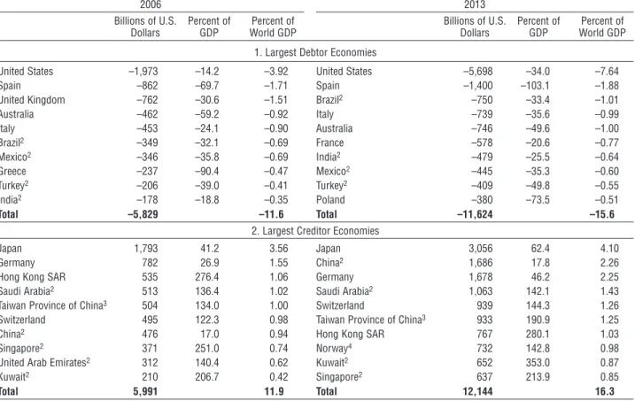
Current account imbalances have narrowed substan-tially since their peak eight years ago, shortly before the global financial crisis (Figure 4.1). At that time, the sum of the absolute values of current account balances across all economies peaked at 5.6 percent of world GDP. Global imbalances subsequently shrank by almost one-third in 2009 at the height of the global recession. They rebounded somewhat in 2010 but have narrowed again since, declining to about 3.6 percent in 2013. Likewise, from 2006 through 2013, the aggregate imbal-ance of the top 10 deficit economies dropped by nearly half as a percentage of world GDP, from 2.3 percent to 1.2 percent (Table 4.1), and the corresponding value for
the top 10 surplus economies dropped by one-fourth, from 2.1 percent to 1.5 percent.
The constellation of deficits and surpluses also changed by 2013 (Table 4.1; Figures 4.2 and 4.3). On the deficit side, the large U.S. deficit shrank by half in dollar terms and by almost two-thirds as a percentage of world GDP. European economies with large defi-cits—though not the focus of initial concerns about imbalances—moved as a whole to a small surplus (Greece, Italy, Poland, Portugal, and Spain). Deficits in some advanced commodity exporters (Australia and Canada) rose, and those of some major emerging mar-ket economies (Brazil, India, Indonesia, Mexico, and Turkey), some of which had run surpluses in 2006,
–3 –2 –1 0 1 2 3 4
1980 85 1990 95 2000 05 10 13
United States Europe surplus Rest of world China Europe deficit Discrepancy Germany Other Asia
Japan Oil exporters
Source: IMF staff calculations.
Note: Oil exporters = Algeria, Angola, Azerbaijan, Bahrain, Bolivia, Brunei Darussalam, Chad, Republic of Congo, Ecuador, Equatorial Guinea, Gabon, Iran, Iraq, Kazakhstan, Kuwait, Libya, Nigeria, Norway, Oman, Qatar, Russia, Saudi Arabia, South Sudan, Timor-Leste, Trinidad and Tobago, Turkmenistan, United Arab Emirates, Venezuela, Yemen; Other Asia = Hong Kong SAR, India, Indonesia, Korea, Malaysia, Philippines, Singapore, Taiwan Province of China, Thailand. European economies (excluding Germany and Norway) are sorted into surplus or deficit each year by the signs (positive or negative, respectively) of their current account balances.
Current account imbalances have narrowed substantially since their peak eight years ago, and their configuration has changed markedly.
Figure 4.1. Global Current Account (“Flow”) Imbalances (Percent of world GDP)
moved up to occupy the remaining top 10 spots.4
Overall, the concentration of deficits also fell dramati-cally: in dollar terms, the top 5 economies in 2006 accounted for 80 percent of the global deficit; in 2013, the top 5 accounted for less than 65 percent of the (reduced) total.
On the other side, China’s surplus almost halved in relation to world GDP, putting it second to that of Germany. Also especially notable is Japan, nearly tied for second place in 2006 but absent from the top 10 in 2013. Major factors behind the decline of China’s surplus were sharply higher investment, expansionary fiscal policy in response to the global financial crisis, booms in credit and asset prices, and lower external demand—all of which were reflected in substantial nominal and real effective exchange rate apprecia-tion. Japan’s trade balance moved into deficit for the
4See Chapter 1 of the October 2014 Global Financial Stability
Report, which focuses on the growth of U.S. dollar corporate liabili-ties and private sector leverage in these emerging market economies, underlining that in most cases, the larger debtor positions have not been accompanied by larger fixed investments and higher growth.
first time since 1980, in part because of higher energy imports after the Great East Japan earthquake, the disruption to exports after the earthquake as well as the Thai floods, and increased public spending since the crisis. The surpluses of some European economies (Ger-many, Netherlands, Switzerland), by contrast, together with those of oil exporters, remained large.5 Although
Norway and Russia (and Singapore) dropped out of the top 10, Qatar and the United Arab Emirates joined that group, along with the Republic of Korea and Tai-wan Province of China. The share of the top 5 econo-mies in the global dollar surplus barely changed, with those economies accounting for about half the total.
Therefore, in the most recent picture, the overall constellation of global imbalances looks quite different than that in 2006. What brought about this change and whether the narrowing of the imbalances is likely to persist are the subjects of the next two sections.
5For at least some oil exporters, current account surpluses are
insufficient from an intergenerational equity perspective.
Table 4.1. Largest Deficit and Surplus Economies, 2006 and 2013
2006 2013
Billions of U.S.
Dollars Percent of GDP World GDPPercent of Billions of U.S. Dollars Percent of GDP World GDPPercent of 1. Largest Deficit Economies
United States –807 –5.8 –1.60 United States –400 –2.4 –0.54
Spain –111 –9.0 –0.22 United Kingdom –114 –4.5 –0.15
United Kingdom –71 –2.8 –0.14 Brazil –81 –3.6 –0.11
Australia –45 –5.8 –0.09 Turkey –65 –7.9 –0.09
Turkey –32 –6.0 –0.06 Canada –59 –3.2 –0.08
Greece –30 –11.3 –0.06 Australia –49 –3.2 –0.07
Italy –28 –1.5 –0.06 France –37 –1.3 –0.05
Portugal –22 –10.7 –0.04 India –32 –1.7 –0.04
South Africa –14 –5.3 –0.03 Indonesia –28 –3.3 –0.04
Poland –13 –3.8 –0.03 Mexico –26 –2.1 –0.03
Total –1,172 –2.3 Total –891 –1.2
2. Largest Surplus Economies
China 232 8.3 0.46 Germany 274 7.5 0.37
Germany 182 6.3 0.36 China 183 1.9 0.25
Japan 175 4.0 0.35 Saudi Arabia 133 17.7 0.18
Saudi Arabia 99 26.3 0.20 Switzerland 104 16.0 0.14
Russia 92 9.3 0.18 Netherlands 83 10.4 0.11
Netherlands 63 9.3 0.13 Korea 80 6.1 0.11
Switzerland 58 14.2 0.11 Kuwait 72 38.9 0.10
Norway 56 16.4 0.11 United Arab Emirates 65 16.1 0.09
Kuwait 45 44.6 0.09 Qatar 63 30.9 0.08
Singapore 37 25.0 0.07 Taiwan Province of China 58 11.8 0.08
Total 1,039 2.1 Total 1,113 1.5
The Mechanics of the Adjustment
In principle, external adjustment can take place through changes in aggregate expenditure or changes in its composition. In practice, adjustment in deficit economies often takes place through expenditure reduc-tion. That is certainly the case for the 2006–13 period (see, for example, Lane and Milesi- Ferretti 2014). This has meant that the squeeze in external (flow) imbal-ances was accompanied by a substantial widening of internal imbalances, that is, greater economic slack (to the extent that the declines in output in deficit econo-mies have been cyclical, driven only by temporarily low demand). In a number of deficit economies, mostly advanced, the adjustment took place amid the typical legacy of financial crisis: a downshift in the path of output relative to precrisis trends (approximated by the medium-term output forecasts from the October 2006
World Economic Outlook).
The panels in Figure 4.4—which show a number of key variables for the main individual deficit and surplus economies established in Table 4.1, as well as
for various groups of economies—highlight the down-shift in output for the United States and European deficit economies. The output contractions were highly synchronized across advanced economies, in deficit and surplus economies alike, as were the declines in output paths. Nevertheless, the output contractions and downshifts were typically smaller, relatively speaking, in surplus economies, which experienced only mild financial crises, if any, and were mostly hit by spill-overs. In China and other emerging market economies, output remained close to precrisis trends.
If the reduction in demand and output in deficit economies was the main mechanism for the post-2006 adjustment in global imbalances (and trade spillovers one of the transmission mechanisms), one would expect to see a relatively stronger export contraction in major surplus economies. This was indeed the case in China and oil exporters, and to a lesser extent in Japan, where exports contracted more than imports. The relatively stronger economic conditions in surplus
Current account deficit,
2013
Current account deficit, 2006 Increasing imbalances
Decreasing imbalances
–3 –2 –1 0 1 2 3 4 5 6 7 8 9 10 11 12 13 14 15
0 1 2 3 4 5 6 7 8 9 10 11 12 13 14 15 MEX
IND
FRA POL
ZAF
PRT
ITA GRC
TUR
AUS GBR
ESP USA
Source: IMF staff estimates.
Note: Size of bubble is proportional to the share of the economy in world GDP. Data labels in the figure use International Organization for Standardization country codes.
The large U.S. deficit shrank by more than half as a percent of its own GDP between 2006 and 2013. The largest European deficit economies also moved as a whole to a small surplus.
Figure 4.2. Largest Deficit Economies, 2006 and 2013 (Percent of GDP)
–5 0 5 10 15 20
0 2 4 6 8 10 12 14 16 18 20
IDN CAN BRA
TWN
ARE
KOR
NOR CHE
NLD
RUS JPN
DEU
CHN
Current account surplus,
2013
Current account surplus, 2006 Increasing imbalances
Decreasing imbalances
Source: IMF staff estimates.
Note: Size of bubble is proportional to the share of the economy in world GDP. Data labels in the figure use International Organization for Standardization country codes. Kuwait, Qatar, and Saudi Arabia are outliers and are not shown.
The large current account surpluses in China and Japan fell substantially as a percentage of national GDP between 2006 and 2013. A number of northern European and advanced Asian economies were running even greater surpluses by 2013, while some major emerging market economies moved from surpluses to deficits.
Figure 4.3. Largest Surplus Economies, 2006 and 2013 (Percent of GDP)
Figure 4.4. Key Indicators of External Adjustment, 2006 Episode (Index, 2006 = 100 unless noted otherwise)
Source: IMF staff calculations.
Note: Europe deficit = Albania, Bosnia and Herzegovina, Bulgaria, Croatia, Cyprus, Czech Republic, Estonia, France, Greece, Hungary, Iceland, Ireland, Italy, Kosovo, Latvia, Lithuania, FYR Macedonia, Malta, Montenegro, Poland, Portugal, Romania, Serbia, Slovak Republic, Slovenia, Spain, Turkey, United Kingdom; Europe surplus = Austria, Belgium,
Real domestic demand Real domestic demand forecast, September 2006 WEO
Saving Investment
Real effective exchange rate Terms of trade
Real exports Real imports
Real GDP Real GDP forecast, September 2006 WEO
70 85 100 115 130 145 160
2004 07 10 13
70 85 100 115 130 145 160
2004 07 10 13
60 95 130 165 200
2004 07 10 13
70 85 100 115 130 145 160
2004 07 10 13
–5 –4 –3 –2 –10 1 2 3 70 85 100 115 130 145 160
2004 07 10 13
70 85 100 115 130 145 160
2004 07 10 13
–5 –4 –3 –2 –1 0 1 2 3 70 85 100 115 130 145 160
2004 07 10 13
70 85 100 115 130 145 160
2004 07 10 13
70 85 100 115 130 145 160
2004 07 10 13
–1 0 1 2 3 4 5 6 7 70 85 100 115 130 145 160
2004 07 10 13 60
95 130 165 200
2004 07 10 13
20. China 19. Germany
18. Europe Deficit 17. United States
12. China 11. Germany
10. Europe Deficit 9. United States
16. China 15. Germany
14. Europe Deficit
4. China 3. Germany
2. Europe Deficit
13. United States 1. United States
Gross Domestic Product
Trade
Real Effective Exchange Rate and Terms of Trade
Saving and Investment (percent change in country/group GDP, 2006–13)
70 85 100 115 130 145 160
2004 07 10 13 70
85 100 115 130 145 160
2004 07 10 13
70 85 100 115 130 145 160
2004 07 10 13 60
95 130 165 200
2004 07 10 13
8. China 7. Germany
6. Europe Deficit 5. United States
Domestic Demand 70 85 100 115 130 145 160
2004 07 10 13
–5 –4 –3 –2 –1 0 1 2 3
Figure 4.4. Key Indicators of External Adjustment, 2006 Episode (continued) (Index, 2006 = 100 unless noted otherwise)
Denmark, Finland, Luxembourg, Netherlands, Sweden, Switzerland; Other Asia = Hong Kong SAR, India, Indonesia, Korea, Malaysia, Philippines, Singapore, Taiwan Province of China, Thailand; Oil exporters = Algeria, Angola, Azerbaijan, Bahrain, Bolivia, Brunei Darussalam, Chad, Republic of Congo, Ecuador, Equatorial Guinea, Gabon, Iran, Iraq, Kazakhstan, Kuwait, Libya, Nigeria, Norway, Oman, Qatar, Russia, Saudi Arabia, South Sudan, Timor-Leste, Trinidad and Tobago, Turkmenistan, United Arab Emirates, Venezuela, Yemen. –10 –8 –6 –4 –2 0 2
Real domestic demand Real domestic demand forecast, September 2006 WEO
Saving Investment
Real GDP Real GDP forecast, September 2006 WEO
70 85 100 115 130 145 160
2004 07 10 13
70 85 100 115 130 145 160
2004 07 10 13
70 85 100 115 130 145 160
2004 07 10 13
70 85 100 115 130 145 160
2004 07 10 13
70 85 100 115 130 145 160
2004 07 10 13
–10 –8 –6 –4 –2 0 2 70 85 100 115 130 145 160
2004 07 10 13
70 85 100 115 130 145 160
2004 07 10 13
–10 –8 –6 –4 –2 0 2 70 85 100 115 130 145 160
2004 07 10 13
70 85 100 115 130 145 160
2004 07 10 13
70 85 100 115 130 145 160
2004 07 10 13
–6 –4 –2 0 2 70 85 100 115 130 145 160
2004 07 10 13 70
85 100 115 130 145 160
2004 07 10 13
40. Oil Exporters 39. Other Asia
38. Europe Surplus 37. Japan
32. Oil Exporters 31. Other Asia
30. Europe Surplus 29. Japan
36. Oil Exporters 35. Other Asia
34. Europe Surplus
24. Oil Exporters 23. Other Asia
22. Europe Surplus
33. Japan 21. Japan
Gross Domestic Product
Saving and Investment (percent change in country/group GDP, 2006–13)
70 85 100 115 130 145 160
2004 07 10 13 70
85 100 115 130 145 160
2004 07 10 13
70 85 100 115 130 145 160
2004 07 10 13 70
85 100 115 130 145 160
2004 07 10 13
28. Oil Exporters 27. Other Asia
26. Europe Surplus 25. Japan
Domestic Demand
Real effective exchange rate Terms of trade
Real Effective Exchange Rate and Terms of Trade
economies thus broadly led to some demand rebalanc-ing between deficit and surplus economies.
Weak domestic demand mainly reflected a sharp contraction in investment expenditure in most econo-mies, but more so for deficit economies than for those in surplus. This, in turn, helped narrow the current account imbalances of advanced deficit economies (for example, the United States and a number of European deficit economies) and at the same time improved the financial net lending and borrowing positions of households and nonfinancial corporations. Although aggregate investment also fell in advanced surplus economies (for example, Japan and several northern European economies), this decline was more than offset by a reduction in aggregate saving, which led to an overall narrowing of their surpluses.6 In contrast,
China, the largest surplus economy in 2006, expe-rienced a significant increase in investment, which, compounded by a small decline in national saving, resulted in a substantial narrowing of its current account surplus.7
Such rebalancing continued because many surplus economies, emerging market economies in particular, recovered faster from the global financial crisis than advanced economies in deficit. The sources of the dif-ferential reflected not only macroeconomic policy stim-ulus, notably in China, but also strong capital inflows, the rebound in commodity markets, and gains in terms of trade, which also boosted domestic demand.
These growth differentials supported further demand rebalancing, leading to relatively faster growth of import volumes and a rising divergence of the path for export volume from that for import volume. Current account surpluses declined, with some major emerging market economies experiencing current account reversals. Oil exporters were the main exception; their current account balances improved with higher oil prices, notwithstand-ing rapid import growth. The flip side to the risnotwithstand-ing terms of trade for commodity exporters was terms-of-trade losses in commodity importers, including in deficit economies; all else equal, the terms-of-trade losses
6Germany was the exception, with a relatively larger decrease
in overall investment relative to saving, leaving it as the only large surplus economy to experience a widening of its surplus.
7Much of the increase in the investment-to-GDP ratio (5.5
per-centage points) took place during the period 2006–09. The saving rate also increased during this period, partly offsetting the impact on the current account surplus, which fell by 3.5 percentage points. Since 2009 the saving rate has declined and the investment-to-GDP ratio has increased modestly, with a further 2.8 percentage point adjustment in the current account.
lowered the improvements in external current accounts in nominal terms or as a percentage of GDP.
Real currency appreciation in some surplus econo-mies and depreciation in some deficit econoecono-mies suggest that some expenditure switching has taken place in the recent narrowing of imbalances. Currency appreciation in China, commodity exporters, and emerging market economies stands out on the surplus side; dollar deprecia-tion has helped in the United States. In contrast, there has been little real appreciation in Japan or depreciation in European deficit and European surplus economies. This underscores how pegged currencies and down-ward nominal rigidities in a number of stressed deficit economies, notably in the euro area, have constrained the relative price adjustment needed for the reallocation of resources between tradables and nontradables. The CPI-based real effective exchange rate measure used in the analysis may, however, understate the impact of changes in relative prices on the current account relative to other measures, such as relative unit labor costs. Unfortu-nately, unit-labor-cost-based real effective exchange rates are available only for a relatively limited set of (mostly advanced) economies.
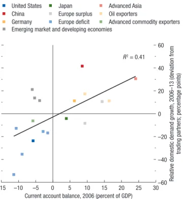
The relationship between a country’s 2006 cur-rent account balance and the subsequent growth in domestic demand relative to that of its trading partners is positive and statistically significant (Figure 4.5). That is, economies with surpluses (deficits) experienced faster (slower) demand growth compared with their partners. The same is true of the subsequent change in the value of currencies (Figure 4.6): economies with surpluses (deficits) experienced real appreciations (depreciations) relative to their trading partners.
Although both expenditure reduction and expenditure switching have been at play, the subsequent adjustment in current account balances has been more strongly related to changes in relative domestic demand (Figure 4.7) than to changes in the real effective exchange rate (Figure 4.8). More formal analysis is afforded by a panel regression of the annual change in the current account (as a share of GDP) on the change in aggregate demand relative to that in trading partners, changes in the real effective exchange rate, and changes in the terms of trade. The regression yields statistically significant coefficients with the expected sign for all explanatory variables.8 The R2 of
8The panel consists of 64 economies for the period 1970–2013;
see Appendix 4.2 for details. The real effective exchange rate is potentially endogenous to the current account, which tends to bias the coefficient downward, so the finding of a statistically significant negative coefficient is despite, not because of, any endogeneity bias.
the regression (including lags of all explanatory variables) is 0.41; dropping the aggregate demand terms lowers it to 0.10, but dropping the real effective exchange rate term lowers it only to 0.39. In other words, the real effective exchange rate, though statistically significant, adds little to the explanatory power of the regression. For the 2007–13 period, the relative importance of the demand terms is even more apparent: the (implied) R2 of the full model
for this period is 0.51; without the demand terms it is 0.02, and without the real effective exchange rate term, it is 0.51. The importance of expenditure reduction in the recent adjustment can also be gauged by comparing the implied 2013 level of aggregate (surplus and deficit) global imbalances with, and without, the effect of the real
effective exchange rate movement; the latter is higher by only 0.4 percent of world GDP, while the overall reduc-tion in imbalances for the 64 economies in the sample was 2.7 percent of world GDP.
The limited explanatory power of the real effec-tive exchange rate in the current account adjustment reflects a number of factors beyond the generally domi-nant role of demand changes in a global crisis context. Structural and institutional factors limited real effective exchange rate adjustment in some cases, notably within the euro area.9 In the case of the United States and
Japan, shocks to domestic energy production may
9On implications of the nominal exchange rate regime for the
persistence of current account imbalances, see Ghosh, Qureshi, and Tsangarides 2014.
Source: IMF staff calculations.
Note: The deviation of domestic demand growth from that of trading partners is calculated as the difference between the deviation of real domestic demand growth (2006–13) from its preadjustment trend (1996–2003) and the deviation of domestic demand growth in trading partners (2006–13) from its preadjustment trend (1996–2003). Advanced commodity exporters = Australia; Advanced Asia = Singapore; Emerging market and developing economies = Poland, South Africa, Turkey; Europe deficit = Greece, Italy, Portugal, Spain, United Kingdom; Europe surplus = Netherlands, Switzerland; Oil exporters = Norway, Russia.
Economies with surpluses (deficits) in 2006 typically experienced faster (slower) domestic demand growth relative to that of their trading partners between 2006 and 2013.
Figure 4.5. Growth of Domestic Demand Relative to Trading Partners versus 2006 Current Account
0 20 40 60
–15 –10 –60
–40 –20
–5
– 0 5 10 15 20 25 30
Current account balance, 2006 (percent of GDP)
R2 = 0.41 United States Japan Advanced Asia China Europe surplus Oil exporters
Germany Europe deficit Advanced commodity exporters Emerging market and developing economies
Rela
tive domestic demand gro
wth,
2006–13 (devia
tion from
trading partners; percenta
ge points)
Source: IMF staff calculations.
Note: CPI = consumer price index. Advanced commodity exporters = Australia; Advanced Asia = Singapore; Emerging market and developing economies = Poland, South Africa, Turkey; Europe deficit = Greece, Italy, Portugal, Spain, United Kingdom; Europe surplus = Netherlands, Switzerland; Oil exporters = Norway, Russia.
Economies with surpluses (deficits) in 2006 typically experienced real appreciations (depreciations) relative to that of their trading partners between 2006 and 2013.
Figure 4.6. Change in Real Effective Exchange Rate (CPI Based) versus 2006 Current Account
(Percent)
R2 = 0.19 United States Japan Advanced Asia China Europe surplus Oil exporters
Germany Europe deficit Advanced commodity exporters
–20 –10 0 10 20 30 40
–15 –10 –5 0 5 10 15 20 25 30
Current account balance, 2006 (percent of GDP) Emerging market and developing economies
Change in real effective exchange ra
te (CPI based),
2006
have weakened the relation between exchange rate changes and current account adjustment. In the case of the United States, for example, increased produc-tion of tight oil led to current account improvements, while the underlying equilibrium exchange rate likely appreciated. Finally, changes in investor sentiment have sometimes worked against real effective exchange rate realignment, including, for example, in the case of safe haven flows.
The 2006–13 episode is not, of course, the first time that global imbalances have contracted: previous occa-sions include 1974 and 1986. The latter provides an instructive contrast with the current instance (Box 4.1): the real effective exchange rate pictures were broadly similar, with the yen appreciating substantially in real
effective terms in that episode while the dollar depreci-ated. No other currencies changed notably in real effec-tive terms. In the former West Germany, for example, real appreciation began only with reunification in 1990. If anything, the reach of exchange rate changes has been broader in the current episode, with the currencies of major emerging market economies and commodity exporters also appreciating.
The main difference between these adjustment epi-sodes is in the growth environment. Whereas in 1986 the narrowing of imbalances took place in the context of growth rotating above preadjustment trends, the narrowing in the current instance has occurred in the context of the global financial crisis, with likely per-manent losses in output levels and, in some cases, even
Source: IMF staff calculations.
Note: CPI = consumer price index. Advanced commodity exporters = Australia; Advanced Asia = Singapore; Emerging market and developing economies = Poland, South Africa, Turkey; Europe deficit = Greece, Italy, Portugal, Spain, United Kingdom; Europe surplus = Netherlands, Switzerland; Oil exporters = Norway, Russia.
Expenditure switching also was at work in current account adjustment between 2006 and 2013. Economies with depreciated (appreciated) currencies typically experienced an improvement (deterioration) in their current account balances.
Figure 4.8. Changes in Real Effective Exchange Rate and Current Account
–20 –10 –10
–5
R2 = 0.17
0 5 10 15
0 10 20 30 40
Change in current account,
2006–13 (percent of GDP)
Change in real effective exchange rate (CPI based), 2006 versus 2013 (percent)
Emerging market and developing economies
United States Japan Advanced Asia China Europe surplus Oil exporters
Germany Europe deficit Advanced commodity exporters
Source: IMF staff calculations.
Note: Advanced commodity exporters = Australia; Advanced Asia = Singapore; Emerging market and developing economies = Poland, South Africa, Turkey; Europe deficit = Greece, Italy, Portugal, Spain, United Kingdom; Europe surplus = Netherlands, Switzerland; Oil exporters = Norway, Russia.
Expenditure reduction played an important role in current account adjustment between 2006 and 2013. Economies with a larger (smaller) contraction in domestic demand relative to that of their trading partners typically experienced a larger (smaller) improvement in their current account balances.
Figure 4.7. Changes in Domestic Demand and Current Account
–60 –40 –20 –10
–5
R2 = 0.67
0 5 10 15
0 20 40 60
Change in current account,
2006–13 (percent of GDP)
Relative domestic demand growth, 2006–13 (deviation from trading partners; percentage points)
Emerging market and developing economies
United States Japan Advanced Asia China Europe surplus Oil exporters
lower trend growth. Not surprisingly, demand reduc-tion has contributed more to the recent narrowing than in 1986, and expenditure switching correspond-ingly less.
Juxtaposing the external adjustment of the worst-affected East Asian crisis economies in the late 1990s with that of four of the euro area economies most severely affected by the recent crises provides another useful comparison (Box 4.2). Massive and sustained real depreciations, together with a supportive external environment, allowed the East Asian economies to benefit from expenditure switching. By contrast, the four stressed euro area economies during the current episode have experienced only limited expenditure switching so far: the adjustment of relative prices through internal devaluation has been gradual and more painful, hurting their growth prospects (see, for instance, Tressel and others 2014).10 The narrowing of
global imbalances during the current episode is thus bracketed by the two extremes of the East Asian and the euro area experiences.
Overall, the limited role of exchange rate adjust-ments in the narrowing of imbalances has meant that that process has entailed high economic and social costs—most notably, high rates of unemployment and large output gaps—partly because resources were not quickly reallocated between tradables and nontradables sectors. However, it has also allowed for substantial adjustment without disruptive exchange rate adjust-ments to the major reserve currencies (most notably, the dollar) that some feared before the global financial crisis. In the process, the distortions underlying the large imbalances up to about 2006, that is, asset price bubbles and credit booms in many advanced econo-mies, have also largely corrected—though others may have emerged, including because of the expansionary policies that the crisis has engendered.
The Durability of the Adjustment
How lasting is the observed narrowing of current account imbalances likely to be? There are two ele-ments to this question. Mechanically, as activity recov-ers and output gaps start to close, domestic demand will rebound in deficit economies; the concern is that without sufficient expenditure switching, this rebound
10See Berger and Nitsch 2014 and Ghosh, Qureshi, and
Tsanga-rides 2014 for evidence that imbalances within the euro area became more persistent with the adoption of the euro.
could lead to a renewed widening of external imbal-ances.11 Going beyond such mechanics, it is worth
asking whether the policy and other distortions that underlie global imbalances have diminished, especially because—other than the risk of a sudden stop—it is these distortions that carry implications for multilateral welfare. Moreover, inasmuch as policy and other dis-tortions do not—or should not—reappear, the extent to which they have diminished speaks to the durability of the observed adjustment.
Output Gaps and Imbalances
Whether global imbalances will, in the absence of further expenditure switching, again expand as the recovery gets under way is closely linked to the issue of whether output declines in deficit economies since the global financial crisis have been largely cyclical or structural. Experience from past financial crises suggests that potential output often declines and the country never recovers its precrisis growth path (see Cerra and Saxena 2008), but it is extraordinarily dif-ficult to arrive at a definitive judgment—especially in regard to what happens after a far-reaching global financial crisis.
To determine the sensitivity of estimates of the extent to which the observed narrowing of flow imbal-ances will reverse as output gaps close, Figure 4.9 presents different scenarios using alternative assump-tions about output gaps, estimates of which are subject to sizable uncertainty.12 Between 2006 and 2013,
global imbalances shrank by some 2.8 percent of world GDP.13 In a counterfactual scenario,
mechani-cally setting the estimated 2013 output gaps from the
World Economic Outlook (WEO) for the Group of
Twenty economies to zero and comparing the
cycli-11As noted previously, in the aggregate, real effective exchange rate
movements have played only a minor role in the adjustment process to date—though there are some important individual exceptions; for instance, China’s real effective exchange rate has appreciated by some 30 percent since 2007.
12This analysis was undertaken by Vladimir Klyuev and Joong
Shik Kang; see Appendix 4.4 and Kang and Klyuev, forthcoming, for details.
13The sensitivity analysis is based on alternative assumptions
about the output gaps of the Group of Twenty economies. Both in 2006 and in 2013, these economies accounted for more than three-quarters of global deficits and about one-half of global surpluses. The four largest economies—China, Germany, Japan, and the United States—accounted for 60 percent of total deficits and 40 percent of total surpluses in 2006 and 35 percent of total deficits and 31 percent of total surpluses in 2013.
cally adjusted global imbalance in 2013 with the actual level in 2006 yields a narrowing of 2.6 percent of world GDP (Figure 4.9, panel 1).14 The implication is
that virtually all of the narrowing of global imbalances observed to date should be durable and should not reverse as output gaps close.
14Economies are classified as surplus or deficit based on their
positions in 2006. Therefore, the adjustment of global imbal-ances reported in this section differs somewhat from that reported elsewhere in this chapter, where economies are classified as surplus or deficit according to their position each year.
This surprisingly modest estimate for the cyclical component of the global imbalances derives from the synchronicity of output gaps across economies (because it is the difference in output gaps that matters) and from the fact that the output gaps themselves are (relatively) small. In particular, in the WEO data, the economies that saw the greatest declines in output relative to precrisis trends also experienced the largest slowdowns in potential output growth, compressing the range of output gaps.
An alternative view is that an economy’s capacity to produce cannot simply be destroyed in a financial crisis, whereas a sharp increase in uncertainty, pes-simistic expectations, disruption of financing, and other factors could lead to large, but still temporary, decreases in demand. An extreme version of this view is that the full extent of the deviation of out-put from the 2013 level that would be implied by precrisis trends represents the output gap. Applying this alternative assumption naturally gives signifi-cantly larger cyclically adjusted global imbalances for 2013: a deficit of 1.8 percent of world GDP and a surplus of 2.3 percent of world GDP, for a total imbalance of 4.1 percent of world GDP (Figure 4.9, panel 2). The improvement in global imbalances since 2006 would then amount to only 1.5 percent of world GDP. Thus, in this scenario, almost half of the observed adjustment could be undone as output gaps close.
It turns out, however, that it is mainly the U.S. economy that is critical to this calculation. The WEO output gap for the United States in 2013 is 3.8 percent, whereas the trend-based alternative would imply a gap of 10.7 percent, which seems implausible and is hard to reconcile with, for example, improving labor market indicators. Returning to the WEO gap for the United States (keeping all others at their trend deviation gaps) in the counterfactual simulation, or returning to the WEO gaps for both the United States and China, restores the narrowing in the cyclically adjusted global imbalances since 2006 to about 2 per-cent of world GDP (Figure 4.9, panel 2).
Keeping in mind the sizable uncertainty surround-ing estimates of output gaps (notably but not only for the euro area), this suggests that even under extreme assumptions about the size of output gaps, one-half of the observed shrinkage in global imbalances would remain as these gaps close; a more plausible gap assumption for the United States alone would mean that two-thirds should endure.
Source: IMF staff calculations.
Note: Countries are classified as deficit or surplus based on their 2006 position. The trend is estimated in log of real GDP over the period 1998–2005. CHN = China; USA = United States.
The narrowing of current account imbalances since 2006 is likely to be long lasting, as cyclical factors appear to have played a relatively minor role. Even in the worst-case scenario, which results from estimating output gaps as the difference between the actual level of output in 2013 and the 2013 level extrapolated using precrisis trends, the current account narrowing amounts to around 1½ percent of world GDP (which is almost half the adjustment without cyclical factors).
Figure 4.9. Current Account Balances, Cyclically Adjusted and Unadjusted
(Percent of world GDP)
Surplus, unadjusted Deficit, unadjusted Surplus, adjusted for WEO
output gaps Deficit, adjusted for WEO output gaps
–3 –2 –1 0 1 2 3 4 5 6
2000 02 04 06 08 10 12 13
Surplus, unadjusted Deficit, unadjusted Surplus, adjusted for deviations
from trend except USA and CHN
Deficit, adjusted for deviations from trend except USA and CHN Surplus, adjusted for deviations
from trend Deficit, adjusted for deviations from trend 1.
–4 –3 –2 –1 0 1 2 3 4
2000 02 04 06 08 10 12 13
Distortions and Imbalances
Concerns about global imbalances go beyond just their magnitude: from the outset, a key issue in debates has been the extent to which observed imbalances are mani-festations of underlying policy distortions. A complemen-tary approach to assessing the durability of the correction to date is therefore to ask whether the underlying distor-tions have diminished in the intervening years.
To this end, this section compares observed cyclically adjusted current account balances15 with those predicted
using the IMF’s External Balance Assessment (EBA) framework, which is an empirical model of current account determination. Put differently, the residuals from the EBA regression, also known in this context as “current account gaps,” can be considered an indicator of the proportion of current account balances that can-not be explained by a country’s macroeconomic funda-mentals. They are thus a measure of excessive imbalances reflective of underlying distortions and possibly systemic risks.16 Three important caveats bear emphasizing. First,
determining globally consistent measures of current account gaps remains difficult and is model specific. To the extent that the EBA model omits certain unob-served fundamentals, the residual imputes their effect to distortions. Second, some of the variables in the regression are policy variables, which need not necessar-ily be at desirable or sustainable settings. Although the EBA model in its operational form explicitly corrects for deviations between actual and desirable policies (“policy gaps”), time series of “desirable” policy settings are not available for historical data; in the exercise that follows, therefore, the 2013 estimates of desirable policy settings are applied to 2006 as well.17 Third, even for 2013, IMF
staff assessments of current account gaps (provided in the IMF’s External Sector Report) draw on the EBA-based current account gaps (and in most cases are very similar to them) but also reflect staff judgment.
Figure 4.10 reports the fitted and actual values of the current account for the major economies and
15In what follows, “cyclically adjusted” refers to the WEO output
gaps, not the trend deviation output gaps, which were used only for the alternative scenario for the counterfactual analysis earlier in the chapter.
16These arguments are developed by Blanchard and Milesi-Ferretti
(2012).
17Policy gaps or distortions are deviations of actual policy stances
(that is, fiscal balances, health spending, foreign exchange interven-tion, private credit, and capital controls) from their desirable or appropriate levels (as determined by IMF country desks). At the same time, to ensure global consistency, domestic policies are consid-ered relative to foreign policies.
country groups identified in Figure 4.1, where the regression uses actual policy settings (so the residual abstracts from the effect on the current account of divergences of policies from their desirable values and implicitly captures only nonpolicy distortions).18
Figure 4.11 (panel 1) provides a more direct com-parison of the residuals over time: bubbles (whose
18The EBA methodology has been developed by the IMF’s
Research Department to provide current account and exchange rate assessments for a number of economies from a multilateral perspec-tive. The EBA framework has been operational only since 2011, so data on desirable policies for 2006 are not available. The EBA exer-cise does not cover Middle Eastern oil exporters, so these economies are not included in this analysis.
Source: IMF staff calculations.
Note: Adv. comm. exp. = Advanced commodity exporters (Australia, Canada); CHN = China; DEU = Germany; EBA = External Balance Assessment; EMDE = emerging market and developing economies (Brazil, India, Indonesia, Mexico, South Africa, Turkey); Eur. def. = Europe deficit (Greece, Poland, Portugal, Spain); Eur. sur. = Europe surplus (Netherlands, Switzerland); USA = United States. The country groups are averaged using market weights.
Figure 4.10. Largest Deficit and Surplus Economies: Current Account Gaps
(Percent of GDP, EBA fitted)
“Current account gaps”—the difference (marked as “residual”) between actual current account balances and those predicted using the IMF’s External Balance Assessment framework—in the largest deficit and surplus economies shrank between 2006 and 2013.
–10 –5 0 5 10 15
2006 2013 2006 2013 2006 2013 2006 2013 2006 2013 2006 2013 2006 2013 Fitted current account (2006) Residual (2006) Fitted current account (2013) Residual (2013) Actual current account
EMDE Eur.
def. comm.Adv.
exp. Eur.
magnitude is proportional to the country’s share of world GDP) that lie below the 45-degree line indicate a smaller current account gap in 2013 than in 2006. The general picture that emerges from the analy-sis is that current account gaps tended to decrease between 2006 and 2013 for the largest and systemi-cally most important economies. As such, underly-ing distortions and global risks also became smaller. However, they did not disappear. In particular, whereas the current account gaps for China, European deficit economies, and the United States were close to zero
in 2013, they remained elevated for European surplus economies, including Germany.
The residuals above exclude the estimated effects of policy gaps, which are shown separately in Fig-ure 4.11, panel 2. For a few (mostly emerging market) economies, the estimated effect of policy gaps on current account imbalances is larger in 2013 than it was in 2006. Adding these policy gaps to the residu-als would therefore widen the current account gaps for these economies. In most cases, however, the net contribution of policy gaps to current account gaps either remained roughly constant or diminished between 2006 and 2013.
What policies were behind these improvements in the larger economies? In the United States, despite some improvement in the cyclically adjusted fiscal bal-ance, since it is the difference in the balance relative to other trading partners that matters, the fiscal variable actually results in a slight widening of the policy gap between 2006 and 2013.19 A more telling
improve-ment relates to excesses in the financial sector, which both the bust phase of the boom-bust cycle and tighter regulation have helped reduce.20 The net change in the
U.S. policy gap between 2006 and 2013, therefore, is roughly a wash—and the bubble for the United States in Figure 4.11 (panel 2) lies on the 45-degree line. In China, the policy improvement is captured by slower accumulation of foreign exchange reserves and some relaxation of capital controls, which are the counter-parts to the substantial real effective exchange rate appreciation. The policy gap therefore shrinks signifi-cantly. Not all of the narrowing of the current account surplus is necessarily benign, however. Rather than a decline in saving, much of the change in China’s cur-rent account between 2006 and 2013 comes through an increase in the already-high rate of investment, exacerbating concerns about allocative efficiency and financial stability and raising questions about its
sus-19The U.S. fiscal balance (relative to trading partners) improved
through 2009, then deteriorated between 2010 and 2013, implying little difference between snapshots of 2006 and 2013.
20In the EBA regression, most excesses are captured by the residual
(“distortions”) rather than policy variables such as the quality of financial regulation (which is difficult to quantify in a statistical analysis). The only policy variable proxying such excesses is the growth of the ratio of credit to GDP. This is why the bulk of the improvement in the current account gap for the United States shows up in the regression residual rather than in the effect of the policy gap variable. It is also why it would not be appropriate to make too sharp a distinction between “policy distortions” and “other distor-tions” in the analysis.
Source: IMF staff estimates.
Note: EBA = External Balance Assessment. Size of bubbles is proportional to the share of the economy in world GDP. Points below the 45-degree line indicate a smaller estimated residual in 2013 than in 2006; points above, a larger residual. Optimal policies are available only for 2013 and are assumed to be the same for 2006. Data labels in the figure use International Organization for Standardization country codes.
Current account gaps fell between 2006 and 2013 for the largest and
systemically most important economies. This suggests that underlying distortions and global risks also shrank. The contribution of policy gaps in most economies either narrowed or remained roughly unchanged, with the exception of a few emerging market economies. The latter implies that the current account gaps for these economies were larger than reported.
Figure 4.11. Understanding Changes in Distortions Using External Balance Assessment Regressions, 2006 versus 2013
0 1 2 3 4 5 6 7 8 9 10
0 2 4 6 8 10
USA CHN
DEU
CHE NLD
TUR
ESP POL
ZAF MEX
BRA IDN IND
Absolute value of residual from EBA
regression,
2013
Absolute value of residual from EBA regression, 2006 2. Contribution of Policy Gaps, 2006 versus 2013
Increasing gaps
0 1 2 3 4 5
0 1 2 3 4 5
USA
CHN DEU
CHE
NLD TUR ESP
POLZAF MEX
BRA
IDN IND
Absolute value of polic
y ga
p
contribution,
2013
Absolute value of policy gap contribution, 2006 Decreasing gaps
Decreasing gaps 1. Residual from EBA Regression, 2006 versus 2013
Increasing gaps
–1 –1
tainability. For Germany, the net impact of the policy gap shrinks because the effect of lower excessive credit growth (that is, credit growth greater than the rate of GDP growth) more than offsets the tightening of the fiscal balance (relative to trading partners), which itself contributes to widening Germany’s current account surplus.
Although such analysis can never be definitive (being highly dependent on the model used to identify “fundamentals”), it does suggest that policy and other distortions have diminished along with the observed narrowing of flow imbalances during the past few years. The improvement in global imbalances thus is not only quantitative but rather represents, from a multilateral perspective, a qualitative improvement in welfare.21 Nevertheless, the European deficit
econo-mies’ adjustment difficulties, which have resulted in massive import compression, unemployment, and economic dislocation, point to greater scope for surplus economies—especially, though not exclusively, those in the region—to rebalance their economies and switch expenditure toward foreign-produced goods. Moreover, the conclusion that reduced policy and other distortions have narrowed global imbalances is somewhat at odds with the finding in the preced-ing section that lower demand, largely matched by a decrease in potential output, has been responsible for much of the observed narrowing of global imbal-ances. These two observations may be reconciled to the extent that potential output was artificially high as a result of distortions—or (what amounts to the same thing) that output was above potential ( including because of distortions in the financial sector), and the global financial crisis both resolved the distortions and lowered demand, bringing it more in line with potential output. This can only be a partial explana-tion, however, so the role of policy improvements and lower distortions in accounting for the narrower flow imbalances is likely to be limited.22
21This is not to suggest, of course, that no distortions remain. The
2014 Pilot External Sector Report (IMF 2014) discusses a variety of policies to further align current account balances with underlying fundamentals.
22The low goods and services price inflation in the run-up to the
global financial crisis suggests that output is unlikely to have been much above potential since, in that case, the low observed inflation would have meant that all of the excess demand was falling only on imported goods. Although (for instance) the United States indeed had a large current account deficit, it seems implausible that the excess demand would have fallen exclusively on imported goods.
The Stock Dimension of Imbalances
Going beyond flow analysis, the external balance sheet of a country—its international investment position in the balance of payments statistics—is another important dimension in global imbalances (see, for example, Obst-feld 2012a, 2012b). Economies with large net liability positions, in particular, may become vulnerable to disrup-tive external financial market conditions, including, in the extreme case, the sudden drying up of external financing (sudden stops) (see, for example, Catão and Milesi-Ferretti 2013).23 Both in the global financial crisis and
during the subsequent euro area crisis, such vulnerabilities played a prominent role, as a number of economies expe-rienced sovereign debt problems, sudden stops, or both.
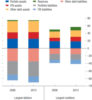
Comparing the 10 largest debtors and 10 largest creditors in 2006 and 2013 reveals striking inertia in these rankings (Table 4.2)—especially compared with those for current account balances (Table 4.1). This inertia exists because net foreign asset stocks are typi-cally slow-moving variables. There is also some overlap between the top 10 list for flow imbalances and that for stock imbalances—which is to be expected, given the two-way feedback between the current account and net foreign asset dynamics (surpluses cumulate into rising stocks; higher net foreign assets generate more factor income, contributing to larger surpluses). The other striking fact about global stock imbal-ances—again, in contrast to flow imbalances—is that they continued to grow during the period 2006–13 (Figure 4.12), with little discernible change in pace after 2006, the year in which flow imbalances peaked. Moreover, they became, if anything, more concentrated on the debtor side, with the share of the top 5 econo-mies rising from 55 percent of world output in 2006 to 60 percent in 2013. The trend of international financial integration has not been reversed, as might have been expected following the global financial crisis (Figure 4.13).
What explains the widening stock imbalances? When these imbalances are measured as a percent-age of GDP, there can be three reasons for wider net foreign asset positions. The first is continued flow imbalances. Even a narrowing of these imbalances, as occurred during the period under consideration, is not enough, all else equal, for a decrease in stock
imbal-23Flow imbalances are sometimes taken as indicating potential
dis-tortions of current policy settings, whereas stock imbalances reflect past policies; stock imbalances may, however, be relevant for current vulnerabilities.
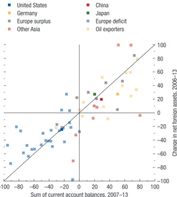
ances. What would be required for such a decrease would be a reversal of flows (from deficit to surplus or vice versa) that is sustained: one year of surplus after several years of deficits will typically not suf-fice. Indeed, there is a strong relationship (R2 = 0.73,
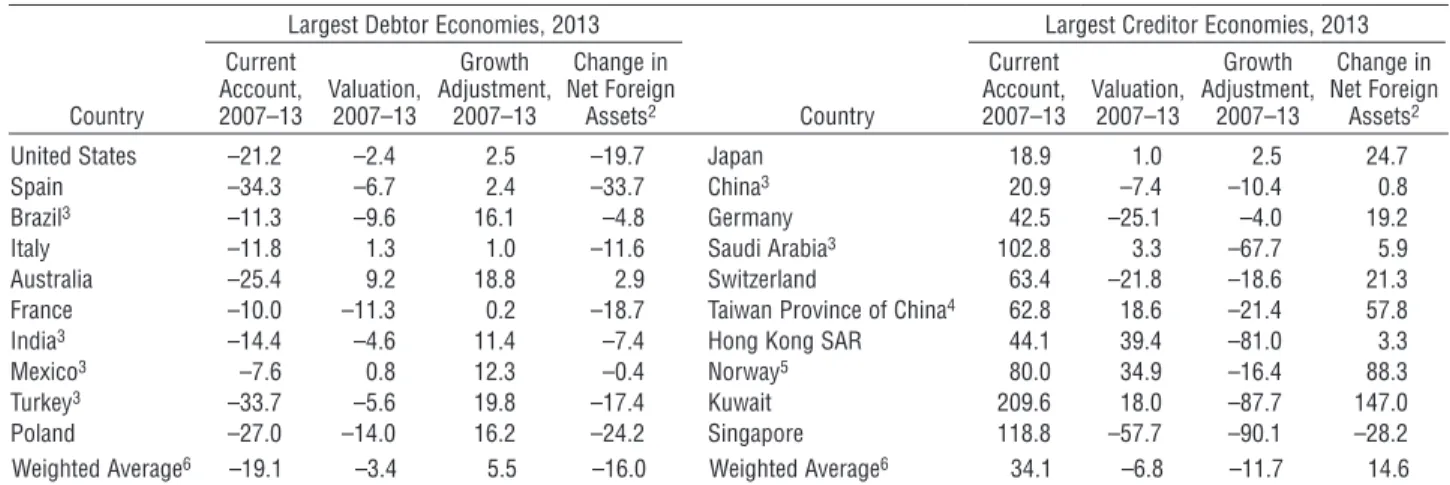
and t-statistic of 13.6) between the change in net foreign assets between 2006 and 2013 and the cur-rent account balances accumulated during the same period (Figure 4.14). On average (and in most of the top 10 cases), continued current account deficits in debtor economies played the main role in the widening stocks of net foreign liabilities as a percentage of GDP (Table 4.3). Similarly, for creditors, continued current account surpluses explain much of the widening stocks of net foreign assets.
Second, valuation effects can change asset positions independently of flow imbalances. Such changes had some effect on net foreign asset positions between 2006 and 2013, albeit in most cases less than those
from cumulative current account balances or eco-nomic growth for the largest debtors and creditors (Table 4.3).24 Notable exceptions were Belgium,
Canada, Finland, Greece, South Africa, and the United Kingdom, where valuation changes were the dominant factor behind the improvement in their net foreign asset positions—and in the United Kingdom’s case, knocked it out of the largest 10 debtors in 2013 (Table 4.2).
The sources of valuation changes are complex and depend on the country’s initial international investment position (creditor or debtor) and the composition of its gross assets and liabilities (fixed income, equity).25 In general, asset prices increased
24See Appendix 4.1.
25A panel regression of 60 economies from 2006 to 2013 suggests
that creditor economies made fewer valuation gains (as a share of their initial stock position) compared with debtor economies. At the same time, nominal depreciation in debtor economies appears to have increased valuation gains for these economies (because it
Table 4.2. Largest Debtor and Creditor Economies (Net Foreign Assets and Liabilities), 2006 and 20131
2006 2013
Billions of U.S.
Dollars Percent of GDP World GDPPercent of Billions of U.S. Dollars Percent of GDP World GDPPercent of 1. Largest Debtor Economies
United States –1,973 –14.2 –3.92 United States –5,698 –34.0 –7.64
Spain –862 –69.7 –1.71 Spain –1,400 –103.1 –1.88
United Kingdom –762 –30.6 –1.51 Brazil2 –750 –33.4 –1.01
Australia –462 –59.2 –0.92 Italy –739 –35.6 –0.99
Italy –453 –24.1 –0.90 Australia –746 –49.6 –1.00
Brazil2 –349 –32.1 –0.69 France –578 –20.6 –0.77
Mexico2 –346 –35.8 –0.69 India2 –479 –25.5 –0.64
Greece –237 –90.4 –0.47 Mexico2 –445 –35.3 –0.60
Turkey2 –206 –39.0 –0.41 Turkey2 –409 –49.8 –0.55
India2 –178 –18.8 –0.35 Poland –380 –73.5 –0.51
Total –5,829 –11.6 Total –11,624 –15.6
2. Largest Creditor Economies
Japan 1,793 41.2 3.56 Japan 3,056 62.4 4.10
Germany 782 26.9 1.55 China2 1,686 17.8 2.26
Hong Kong SAR 535 276.4 1.06 Germany 1,678 46.2 2.25
Saudi Arabia2 513 136.4 1.02 Saudi Arabia2 1,063 142.1 1.43
Taiwan Province of China3 504 134.0 1.00 Switzerland 939 144.3 1.26
Switzerland 495 122.3 0.98 Taiwan Province of China3 933 190.9 1.25
China2 476 17.0 0.94 Hong Kong SAR 767 280.1 1.03
Singapore2 371 251.0 0.74 Norway4 732 142.8 0.98
United Arab Emirates2 312 140.4 0.62 Kuwait2 652 353.0 0.87
Kuwait2 210 206.7 0.42 Singapore2 637 213.9 0.85
Total 5,991 11.9 Total 12,144 16.3
Sources: IMF, World Economic Outlook database; External Wealth of Nations Mark II data set (Lane and Milesi-Ferretti 2007); and Lane and Milesi-Ferretti 2012.
1The External Wealth of Nations Mark II data set (Lane and Milesi-Ferretti 2007) used in this analysis excludes gold holdings from foreign exchange reserves. 2IMF staff estimates for these economies may differ from the international investment position, where reported.
3National sources. 4IMF staff estimates for 2013.
between 2006 and 2013: both equity and bond prices rose with the substantial decline in long-term interest rates, which, all else equal, should benefi t net creditors relative to net debtors (and thus widen imbalances). Conversely, the drastic downward revision of economic prospects for most large debtor economies after the global fi nancial crisis lowered the value of assets located in these economies. Although this implies a negative wealth eff ect for a particular country, it also means a
reduced the value of their liabilities, namely, the assets located in the country), which could have helped stabilize their net foreign asset positions. Although these variables are statistically signifi cant in the panel regression, year-by-year cross-sectional regressions yield no systematic relationship between them. Data on the currency composition of external balance sheets are limited and hence are not examined.
lower value of its foreign liabilities, implying a capital gain. Th e United States was unique in this regard: despite the country being a major debtor and having experienced a large downward revision in its growth prospects, the value of U.S. assets rose because of safe haven concerns, implying a capital loss on its interna-tional investment position.
Th ird, growth eff ects can also lead to higher imbal-ances as a share of GDP, as in the case of public debt (Table 4.3). Economic growth was also important, with the eff ects up to roughly one-third the size of those from cumulative current account balances, and with the oppo-site sign. For creditor economies, GDP growing ahead of net foreign assets lowered net foreign asset ratios, whereas in debtor economies, this contributed to lower net foreign liability ratios. In euro area debtor economies, however, Source: IMF staff calculations.
Note: Oil exporters = Algeria, Angola, Azerbaijan, Bahrain, Bolivia, Brunei Darussalam, Chad, Republic of Congo, Ecuador, Equatorial Guinea, Gabon, Iran, Iraq, Kazakhstan, Kuwait, Libya, Nigeria, Norway, Oman, Qatar, Russia, Saudi Arabia, South Sudan, Timor-Leste, Trinidad and Tobago, Turkmenistan, United Arab Emirates, Venezuela, Yemen; Other Asia = Hong Kong SAR, India, Indonesia, Korea, Malaysia, Philippines, Singapore, Taiwan Province of China, Thailand. European economies (excluding Germany and Norway) are sorted into surplus or deficit each year by the signs (positive or negative, respectively) of their current account balances.
Stock imbalances continued to grow between 2006 and 2013 despite the narrowing in flow imbalances. This reflects the fact that to reduce the former, a sustained reversal in the latter is needed.
Figure 4.12. Global Net Foreign Assets (“Stock”) Imbalances (Percent of world GDP)
–25 –20 –15 –10 –5 0 5 10 15 20
1980 85 1990 95 2000 05 10 13
United States Europe surplus Rest of world China Europe deficit Discrepancy Germany Other Asia
Japan Oil exporters
–20 –40 –60 –80 –100 0 20 40 60 80
2006 2013 2006 2013
Largest debtors Largest creditors Porfolio assets Reserves Other debt liabilities FDI assets Portfolio liabilities
Other debt assets FDI liabilities
Sources: External Wealth of Nations Mark II data set (Lane and Milesi-Ferretti 2007); and Lane and Milesi-Ferretti 2012.
Note: FDI = foreign direct investment. Portfolio is both equity and debt portfolio stocks, and other debt is financial derivatives and other (including bank) investments.
Gross assets and liabilities of the largest debtors and creditors continued to expand between 2006 and 2013, with no reversal in the trend of international financial integration following the global financial crisis.
Figure 4.13. Gross Foreign Assets and Liabilities (Percent of world GDP)