Analysis of the Convergence and
Closed Loop Stability in EDMC
M. Haeri
and H. Zadehmorshed Beik
1In this paper, the convergence and stability conditions of extended DMC in the control of nonlinear SISO and MIMO systems are investigated. The formulations are based on the ordinary DMC in which, with successive linearization of the nonlinear model and new interpretation of disturbance, the nonlinear extension is deduced. In addition, new convergence and stability criteria are derived for SISO and MIMO systems. These criteria include convergence and stability in the case of longer control (M>1) and prediction (P >1) horizons, as well as the nite and
innite sampling time. Finally, the simulation results for a MIMO (33) model, based on a
power unit nonlinear plant, are presented.
INTRODUCTION
Model Predictive Control (MPC) and its industrial applications have become more and more popular during the last few decades 1-3]. MPC refers to a family of controllers that share three basic schemes 4]. In all model predictive controllers, an explicit model is employed to predict the future outputs of the process. This is why they are also categorized in model based control approaches. The control signal is determined, based on an optimization algorithm to optimize an ob-jective function. This property enables the controllers to handle the constraints explicitly during the control design stage. Finally, the calculated control signals are applied, based on the receding horizon strategy, which is why they are also called receding horizon controllers. So far, almost all types of model structure have been employed in MPC. Linear MPC refers to those controllers that use a linear model structure of the process. In the absence of constraints, use of linear models results in a closed form solution to the op-timization problem. However, in constrained linear MPC, a quadratic programming is usually performed. In nonlinear MPC controllers, on the other hand, a nonlinear model of the process is employed. In this
*. Corresponding Author, Department of Electrical En-gineering, Sharif University of Technology, P.O. Box 11365 9363, Tehran, I.R. Iran.
1. Department of Electrical Engineering, Sharif University of Technology, P.O. Box 11365 9363, Tehran, I.R. Iran.
case, the optimization problem does not generally have a closed form solution. Usually, nonlinear program-ming is implemented to obtain results. Nonlinear programming is run, based on either a sequential 5,6] or simultaneous 7,8] strategy. In either case, high computational power is required 9]. This deciency connes application of nonlinear MPC on processes that possess slow dynamics. In order to reduce com-putational requirements, linear approximations have been employed in some designs of nonlinear model predictive controllers. Multi Model adaptive Predictive Control (MMPC) 10], Quadratic Dynamic Matrix Control (QDMC and NLQDMC) 11,12], Extended Dynamic Matrix Control (EDMC) 13,14] and Univer-sal Dynamic Matrix Control (UDMC) 15] have been introduced from this point of view. In the rst three approaches, an approximated linear model is used to predict the eects of future control moves at each sample time. Free response, however, is computed by integrating the nonlinear model equations. While the linear models are determined o line in MMPC, in QDMC and EDMC they are obtained based on the Jacobian and the perturbation methods at each sample time. The main dierence between QDMC and EDMC is the way of computation and consid-eration of the model/process mismatch and external disturbance. In UDMC, linear approximation is im-plemented only in the calculation of the Jacobians during the updating state of the optimization algo-rithm.
consideration of linear 16-21] and nonlinear 22-25] MPC controllers. The backbone of ideas presented in the literature relies on the inniteness of the pre-diction horizon and, therefore, use of the established stability property of the LQ control theory. Because of impracticality, in most cases, the inniteness of the horizon is replaced by the stability constraints (includ-ing terminal constraints) in some improved schemes. Both hard 16,21] and soft constraints 26,27] were considered. By choosing the cost function in MPC as the candidate of the Lyapunov function and showing that it is a non-increasing function, the stability of the closed loop system is proved. The stability is derived for the nominal condition in most cases and is based on the state space model representation of the process, in which states are assumed to be measurable directly or determined through indirect measurements. It is also assumed that the implemented optimization algorithms are converged to the correct solution of the problem.
Due to their conceptual simplicity and lower com-putational requirements, predictive controllers, such as QDMC and EDMC, provide realistic advanced control strategies for industrial applications. It is shown in 12] that by tolerating a negligible loss in the closed loop performance, QDMC was six times faster than a nonlinear MPC run based on the sequential method. Unfortunately, there is not an analytical and explicit stability proof for QDMC or NLQDMC. Nevertheless, stable closed loop behavior has been illustrated in computer simulations, as well as actual implementation of the controllers, even for open loop integrating, as well as unstable processes 9,11,12]. To get a stable closed loop system, the state space representation of the process, along with a state es-timator, has been employed in NLQDMC 12]. On the other hand, EDMC has proved to be stable, provided that some conditions on the control param-eters and the steady state gain of the process are satised 13]. Proof of the convergence in the internal loop, as well as closed loop stability, was derived based on the contraction mapping theorem. Input/output representations of the process and the controller are used in the formulation of the problem. Imposing unrealistic conditions, such as innite sample time and restricting assumptions, such as unity control and prediction horizons, make the mentioned proof unacceptable in practice. In this paper, the authors try to extend the applicability of the proof by relaxing the above mentioned restricting conditions. In this way, a nonlinear MPC (or time varying linear MPC) has been provided with less computational require-ments, as well as acceptable and realistic stability conditions.
The paper is organized as follows. First, the DMC and its nonlinear extension are reviewed and
nonlinear vector equations and some powerful solutions are presented. Then, the convergence and closed loop stability conditions for a SISO process case with
M > 1, for nite and innite sampling time, are
proposed. After that, the EDMC formulation for the MIMO system is derived and the related con-vergence theorem and the stability criteria are pre-sented, respectively. Finally, the simulation results for a nonlinear model (33) of a power unit plant
are illustrated. Conclusions are given in the last section.
DMC FORMULATION AND ITS
NONLINEAR EXTENSION FOR SISO
SYSTEMS
Since EDMC formulation is based on ordinary DMC, a brief description of both controllers is presented in this section.
DMC
Considering a SISO system step response model, the output could be determined using the following discrete convolution:
y lin(
k) =
N
X
i=1
aiu(k;i) +aNu(k;N;1) +d(k)
(1) where u(k) and u(k) are the input and its variation
i.e. u(k);u(k;1) in sample timek, respectively. aiis
the step response coecient at sample timei. N is the
number of sample time at which step response reaches its steady state. The following disturbance represents any dierence between the measured output and the one predicted by the above model:
d(k)=ymeas(k);
N
X
i=1
aiu(k;i);aNu(k;N;1):
(2) The future predictions of the process output are given in the following matrix-vector relation:
2 6 6 6 4 y
lin( k+ 1) y
lin( k+ 2)
...
y lin(
k+P) 3 7 7 7 5
=
2 6 6 6 6 6 6 6 6 4 a
1 0 0
0
a 2
a
1 0
0
...
aM aM ;1
a
1
...
ap ap ;1
ap ;M+1
3 7 7 7 7 7 7 7 7 5
2 6 6 6 4
u(k)
u(k+ 1)
... u(k+M;1)
3 7 7 7 5
2 6 6 6 4
a 2
a 3
aN
a 3
a 4
aN 0
...
ap +1
aN 0 3 7 7 7 5
2 6 6 6 4
u(k;1)
u(k;2)
... u(k;N+ 1)
3 7 7 7 5
+
2 6 6 6 4
aNu(k;N) aNu(k;N+ 1)
...
aNu(k;N+P;1) 3 7 7 7 5
+
2 6 6 6 4
d(k+ 1) d(k+ 2)
...
d(k+P) 3 7 7 7 5
: (3)
This can be written, equivalently, in the following vector form:
y
lin=Au
+y
past+d
(4)
P and M are the prediction and moving (control)
horizons, respectively,
y
past denotes the eects of thepast inputs on the predicted outputs.
A
is a Toeplitz matrix, consisting of step response coecients and is called the dynamic matrix of the process. Since future estimates of the mismatches are not available, it is customary to assumed(k+i) =d(k) fori= 12P.The control moves,
u
, are determined according to the solution of the following optimization problem. minu
P
X
i=1
yd(k+i);y lin(
k+i)
2
+XM
j=1
2
u(k+M;j)] 2
(5)
yd is the desired output trajectory and is the
weighting coecient on the input variations. Using least square estimation, the solution of the problem is given by:
u
=;A
TA
+ 2I
;1
A
T;y
d;y
past ;
d
: (6)
Usually, the rst component of
u
, i.e. u(k), willbe applied to the process (u(k) = u(k;1) + u(k))
and the same procedure will be performed in future sampling intervals.
Extended DMC
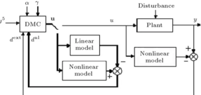
To extend the application of DMC (which is originally based on a linear model of the process) to nonlinear systems, it is required to employ an approximated linear model for a nonlinear process in each sample interval. This is done via linearization of the process's nonlinear model or by determination of the process response for a step perturbation. Also, a new in-terpretation of disturbance is introduced, due to the nonlinear character of the process. This is explained in more detail in the next section.
Nonlinear Disturbance
In this extension, a new interpretation of
d
is ex-ploited 13]. In other words,d
is split into two parts, the unknown parts,d
ext, which are treated asin ordinary DMC and the known parts,
d
nl, whichrepresent the dierence between approximated linear and nonlinear models of the process.
d
=d
ext+d
nl: (7)
To consider this partitioning, the predicted outputs of the process are written as:
y
el=Au
+y
past+d
ext+d
nl(8)
d ext(
k+i) is assumed constant over the prediction
horizon (i = 12P) and d nl(
k+i) varies during
the horizon. Solving Problem 5 results in the following relation for input variations:
u
(d
nl)= ;A
TA
+ 2I
;1
A
T;y
sp;
y
past;
d
ext;
d
nl
(9)
d
nlis determined, in order to have the same predictedoutputs from the nonlinear,
y
nl, and linear,y
el,mod-els,
y
nl(d
nl) =y
el=Au
(d
nl) +y
past+d
ext+d
nl :(10) To solve the above problem, equation 10 is reformu-lated in the following equation, which is a root nding problem:
f
(d
nl)=y
nl(d
nl);
Au
(d
nl);
y
past;
d
nl;
d
ext=0
:
(11) There are P nonlinear equations in P unknowns, d
nl(
k+1)d nl(
k+P). Nonlinearity of the equations
arises from the nonlinear relation that exists between
y
nl andu
(and, therefore,u
). In the followingsub-section, some well established methods are summarized that can be applied to nd the solution to the problem. One of the simplest methods is successive substitution via a xed-point algorithm,
d
nlk+1=
f
1(d
nl
k) =
d
nlk +(
y
nlk ;
y
elk) =
d
nlk +
f
(d
nlk):
(12) A block diagram of EDMC in Figure 1 shows the internal iteration and external DMC closed loop after convergence.
Figure1. Block diagram of EDMC algorithm.
Nonlinear Vector Equation Solution
Almost all existing approaches to nding a solution to a nonlinear vector function, such as
f
(x
) =0
, rely on iterative methods. The Newton method 28] is perhaps one of the most popular and is given by the following relation:x
k+1=x
k ;f
0(
x
k)];1f
(x
k): (13)
This method benets from convergence rate 2 around the optimal solution. However, it requires a Jacobian matrix that is not easily available in most applications, like Problem 11. A simplied version of the Newton method is obtained by substituting
f
0(x
) with a xedmatrix,
C
. Sometimes, the initial value of the Jacobian matrix,f
0(x
0), is used in this regard:x
k+1=x
k ;C
;1
f
(x
k) =x
k ;f
0(
x
0);1f
(x
k) : (14)The xed-point iteration method is obtained by re-placing;
C
;1 with
I
, in which is a small positivecoecient:
x
k+1=x
k+f
(x
k) 2(01): (15)This method requires the least computational eort and benets from a convergence rate of one. Iteration methods given in Equations 12 and 14 have been used in 13] and some good results have been obtained for certain conditions. In Quasi Newton (QN) methods, some approximation of the Jacobian matrix is em-ployed. In Broyden's method 29], the following steps are performed in each iteration:
x
k+1=x
k+s
ky
k=f
(x
k+1);
f
(x
k)w
ks
k =;f
(x
k)w
k+1 =w
k+ (y
k;w
ks
k)s
Tks
Tks
k (16)w
k is an approximate forf
0(x
k) and initialized by
w
0=f
0(x
0). This method converges to the solution at
an approximate rate of 1.6, which means super linear
convergence. Some other methods of the QN family, such as Greenstadt, Barnes and Thomas, can be found in 30].
The two following subsections describe the con-tribution made by the present work. This includes an extension of the work in 13] to higherM and MIMO
systems.
Convergence for SISO Systems with
M >1
As in 13], convergence of the xed-point iterations can be proved via the contraction-mapping theorem. It is shown that for a globally asymptotically stable open loop system, iterations in Equations 9 and 12 will converge if the sampling time and weighting factor are large enough and the relaxation factor,, is small
enough. Since in the above-mentioned conditions, assumption M = 1 is not used, the statement is
also valid for M > 1. With some mathematical
manipulation of the results given in 13], it is shown that the following condition on the weighting factor () is required to get the convergence:
2
>>2MPmax
i fjaiaijg (17)
in which ai and ai are the steady state gain of the
linear and nonlinear models at theith iteration. Since M is allowed to be higher than one, more performance
improvement can be expected from the controller.
Stability for SISO Systems with
M >1
The operator theory and contraction mapping 31] can be used to show the closed loop stability of the system for M > 1 and innite/nite sampling time (T) as
follows.
Innite Sampling Time
In this section, it is required to extend the stability criteria of an SISO system for aM>1 case. Regarding
stability, it is assumed that the iterative computation of
d
nl in sample timek has been converged and the
goal is to derive a relation between present (uk) and
previous (uk
;1) inputs. uk =uk
;1+ uk
=uk ;1+
e
T
1
(
A
TA
+ 2I
);1A
T(y
spk+1 ;
y
past
k+1 ;
d
nl
k+1)
(18)
e
i is a M 1 vector with all elements zero, exceptthe ith element, which is one. Note that for a
nominal system,
d
ext =0
. To complete and simplifyEquation 18, the converged value of
d
nldetermined. When the convergence has been reached, the following equality is satised:
y
nl=y
el
y
nl= y
nl(
k+ 1)y nl(
k+P)]T
and:
y
el = yel(k+ 1)yel(k+P)]T: (19)The output of the extended linear model,
y
elk, is
obtained as follows:
y
elk+1 =
y
pastk+1+
Au
k+d
nlk+1
=
y
pastk+1+
A
(A
T
A
+ 2I
);1A
T(y
spk+1 ;
y
past
k+1 ;
d
nl
k+1) +
d
nlk+1
: (20)
Let one dene:
A
0=A
(A
T
A
+2
I
);1A
T :Using Equations 19 and 20 and the above denition, one can derive the following relation:
(
I
;A
0)d
nl
k+1=
y
nlk+1
;(
I
;A
0)y
past
k+1 ;
A
0
y
spk+1
or:
d
nlk+1=(
I
;A
0) ;1
y
nlk+1 ;
y
past
k+1
;(
I
;A
0);1
A
0y
sp
k+1 :
(21) Substituting
d
nlk from Equation 21 in Equation 18, one
obtains:
uk=uk ;1+
uk
=uk ;1+
e
T
1
(
A
TA
+ 2I
);1A
T(y
spk+1 ;
y
past
k+1
;(
I
;A
0);1
y
nlk+1+
y
pastk+1
+ (
I
;A
0);1
A
0y
sp
k+1)
:
(22) Using the following two matrix relationships for
A
0:(
I
;A
0);1=
I
+ 12
AA
T
(
I
;A
0);1
A
0= 12
AA
T: (23)
Equation 22 is simplied as:
uk=uk ;1+
e
T
1(
A
T
A
+ 2I
);1A
T(I
+ 12
AA
T)(
y
spk+1 ;
y
nl
k+1)
=uk ;1+ 1
2
e
T
1
A
T(
y
spk+1 ;
y
nl
k+1)
: (24)
When considering the innite sampling time assump-tion (T !1), one can use the following denitions:
y
nlk+1 = y
nl(
k+ 1)
1
Py
spk+1= y
sp
1
P
A
=a1
L eT1
A
T
1
P =aP (25)where:
1
P =2 6 6 6 4
1 1 ... 1
3 7 7 7 5
P1
1
L= 2 6 6 6 6 6 6 6 6 41 0 0 0
1 1 0 0
...
1 1 1 1
...
1 1 1 1 3 7 7 7 7 7 7 7 7 5
PM :
(26) Therefore, Equation 24 is further simplied as:
uk=uk ;1+
aP
2( y
sp ;y
nl(
k+ 1)): (27)
This equation is similar to the one derived in 13] but assumptionM = 1 is not used in this case. Therefore,
results given in 13] for the stability of the closed loop system are also applicable to M > 1. This results in
the following theorem. Nominal Stability Theorem
Suppose that the system to be controlled is globally asymptotically stable for all feasible inputs and, fur-thermore, suppose that the following is valid:
1. The steady state gain of the system does not change sign
2. The weight on the change of the input is larger than zero
3. The sampling time is long enough (T!1)
4. The set point is constant in the prediction horizon. Then, the closed loop system is guaranteed to be nominally stable.
Finite Sampling Time
In this section, one considers relaxing assumption 3 in the above stability theory. According to the previous section, this condition is employed in two cases, rst in denitions given in Equation 25 and, second, in deriving the Jacobian of the input in Equation 27. In the following lines, analysis of the stability is continued without considering assumption 3. Recall the relation foruk in Equation 24.
uk=uk ;1+ 1
2
e
T
1
A
T(
y
spk+1 ;
y
nl
k+1)
It is assumed that the internal iteration in EDMC has been converged. This relation is expanded using elements of
e
1A
y
spk+1 and
y
nlk+1: uk =uk
;1+ 1 2
P
X
i=1 ai(y
sp(
k+i);y nl(
k+i)): (29)
To derive the Jacobian of @uk
@uk ;1, derivatives of the
future outputs, with respect touk
;1, are required. @uk
@uk ;1
= 1;
1 2 P X i=1 ai @y nl(
k+i) @uk
;1
= 1;
1 2 a 1 @y nl( k+ 1) @uk ;1 +a 2 @y nl(
k+ 2) @uk
;1
++ap @y
nl( k+P) @uk
;1
:
(30) To solve the problem, the linear approximations of
y nl(
k+i) are used in the computation: y(k+1)=a
1
u(k)+(a 2
;a 1)
u(k;1) + (a 3
;a 2)
u(k;2)
++ (aN;aN ;1)
u(k;N+ 1) y(k+2)=a
1
u(k+1)+(a 2
;a 1)
u(k)+(a 3
;a 2)
u(k;1)
++ (aN;aN ;1)
u(k;N+ 2)
...
y(k+M) =a 1
u(k+M;1) + (a 2
;a 1)
u(k+M;2)
++ (aM +1
;aM)u(k;1)
++ (aN;aN ;1)
u(k;N+M) y(k+M+ 1) =a
2
u(k+M;1)+(a 3
;a 2)
u(k+M;2)
++ (aM +2
;aM +1)
u(k;1)
++ (aN;aN ;1)
u(k;N+M+ 1)
...
y(k+P+ 1) =aP ;M+1
u(k+M;1)+
(aP ;M+2
;aP ;M+1)
u(k+M;2)
++ (aP +1
;aP)u(k;1) +
+ (aN;aN ;1)
u(k;N+P): (31)
Let the following denitions be used:
A
=a
1a
2a
M]and: z 1= @uk @uk ;1 z 2= @uk +1 @uk ;1
zM = @uk
+M;1 @uk
;1 :
(32) Therefore,zi are determined as follows:
z 1= 1
; 1 2
a
T 1 l z 2= z 1 ; 1 2a
T 2l
zM =zM;1 ;
1
2
a
TMl
(33)
l
is a column vector given as:l
= 2 6 6 6 6 6 6 6 6 6 6 6 6 6 6 6 6 4 a 1 z 1+ a 2 ;a 1 a 1 z2+ ( a 2 ;a 1) z 1+ a 3 ;a 2 ... a 1
zM + (a 2 ;a 1) zM ;1+
+ (aM ;aM ;1)
z 1+
aM +1
;aM a
2
zM + (a 3 ;a 2) zM ;1+
+ (aM +1
;aM)z 1+
aM +2
;aM +1
...
aP ;M+1
zM+(aP ;M+2
;ap ;M+1)
zM ;1
++(aP;aP ;1) z 1+ aP +1 ;aP 3 7 7 7 7 7 7 7 7 7 7 7 7 7 7 7 7 5 : (34)
Substitute forziin Equation 34 from Equations 33 and,
with some manipulation,
l
is reformulated as follows:l
= 2 6 6 6 6 4 a 2 ; 1 2 a 1a
T 1l
a 3 ; 1 2( a 2a
T 1 + a 1a
T2)
l
ap+1 ;
1
2( aP
a
T1 +
+aP
+M;1
a
TM)l
3 7 7 7 7 5 : (35) Or, in simple form, it can be written as:l
= ^b
;1
2
^
Bl
(36)where: ^
b
= 2 6 6 6 4 a 2 a 3 ... aP +1 3 7 7 7 5 ^B
= 2 6 6 6 6 6 6 6 4 a 1a
T 1 a 2a
T 1 + a 1a
T 2 aMa
T1 + +a
1
a
TM aM+1
a
T
1 + +a
2
a
TM...
aP
a
T 1 ++aP
+M;1
a
TM 3 7 7 7 7 7 7 7 5 : (37)Equation 36 can be solved for
l
:l
= (I
+ 12
AA
T);1
b
^: (38)
Using the denition of
A
0in the previous section, since(
I
+ 12
AA
T);1 =
I
;A
0, therefore:
l
= (I
;A
0)^
b
= ^b
;A
0
b
^: (39)
From the rst row of Equation 34,z
1 is determined as
follows:
z 1= 1
a 1
(l 1+
a 1
;a 2)
= 1
a 1
(
e
T1l
+ a1 ;a
2)
= 1
a 1
(
e
T1b
^ ;e
T1
A
0b
^+a 1
;a 2)
= 1
a 1
(a 1
;
e
T 1A
0
b
^): (40)
Based on the contraction mapping theorem, closed loop stability requiresz
1
<1. In other words:
1
a 1
e
T1
A
0b
^>0: (41)
Some Special Cases for Stability 1. P =M = 1,
A
0= a1( a
2 1+
2);1
a 1
b
^=a 2
1
a 1
e
T1
A
0b
^= 1a 1
a 2 1 a
2 1+
2
a 2=
a 1
a 2 a
2 1+
2
>0 )a
1 a
2
>0: (42)
2. M= 1P >1,
A
= a1 a
2
aP]T
1
a 1
e
T1
A
0b
^=A
Tb
^AA
T + 2>0
)
A
Tb
^>0: (43)Or, equivalently,
a 1
a 2+
a 2
a 3+
+aPaP +1=
P
X
i=1 aiai
+1 >0:
(44)
3. M= 2P >2
A
TA
+2
I
= Ppi=1 a
2
i + 2
Pp ;1
i=1 aiai
+1 Pp
;1
i=1 aiai
+1 Pp
;1
i=1 a
2
i + 2
(45) 1
a 1
e
T1
A
0b
^= Pp;1
i=1 a
2
i + 2
; Pp
;1
i=1 aiai
+1
det(
A
TA
+ 2l
)2 6 6 4
p
P
i=1 aiai
+1
p;1 P
i=1 aiai
+2 3 7 7 5
=
p;1 P
i=1 a
2
i+ 2
p
P
i=1 aiai
+1
;
p;1 P
i=1 aiai
+1
p;1 P
i=1 aiai
+2
p
P
i=1 a
2
i+ 2
p;1 P
i=1 a
2
i+ 2
;
p;1 P
i=1 aiai
+1
2 >0:
(46)
DMC FORMULATION FOR LINEAR MIMO
SYSTEMS
For the sake of simplicity, formulations are given for 22 systems. The same line of calculations is used
to determine formulas for nn systems. Outputs
of a stable linear time invariant 2 2 system can
be represented, using its step response model, by the following equations:
y 1(
k) =
N
X
i=1 aiu
1(
k;i) +aNu 1(
k;N;1)
+XN
i=1 biu
2(
k;i)+bNu 2(
k;N;1)+d 1(
k)
y 2(
k) =
N
X
i=1 ciu
1(
k;i) +cNu 1(
k;N;1)
+XN
i=1 diu
2(
k;i)+dNu 2(
k;N;1)+d 2(
k)
(47) where ui(k) and ui(k) are the ith input and it's
variation in sample time k. aibici and di are the
step response coecients at sample time i. N is the
sample time at which all the step responses reach their steady state.
d
i stands for any dierencesbetween the system output and the one predicted by the step response model. These errors account for model/system mismatches and external disturbances. Future predictions of the system outputs for prediction horizon P, based on control horizon M, are given in
the following matrix-vector relation: 2 6 6 6 6 6 6 6 6 4 y 1( k+1) ... y 1(
k+P) y 2( k+1) ... y 2(
k+P) 3 7 7 7 7 7 7 7 7 5 = 2 6 6 6 6 6 6 6 6 6 6 6 6 4 a 10 0 b 10 0 a 2 a 10 0 b 2 b 10 0 ...
aPaP ;1
aP ;M+1
bPbP ;1
bP ;M+1 c 10 0 d 10 0 c 2 c 10 0 d 2 d 10 0 ...
cPcP ;1
cP ;M+1
dPdP ;1
dP ;M+1
3 7 7 7 7 7 7 7 7 7 7 7 7 5 2 6 6 6 6 6 6 6 6 6 6 6 6 4 u 1( k) u 1(
k+ 1)
... u
1(
k+M;1)
u 2(
k)
u 2(
k+ 1)
... u
2(
k+M;1) 3 7 7 7 7 7 7 7 7 7 7 7 7 5 + 2 6 6 6 6 6 6 6 6 6 6 6 6 4 a 2 a 3 a 3 a 4 aN +1 ... aP +1 aN +1 c 2 c 3 c 3 c 4 cN +1 ... cP +1 cN +1 aN +1 b 2 b 3 bN +1 0 b 3 b 4 bN +1 0
0 bP +1 bN +1 0 cN +1 d 2 d 3 dN +1 0 d 3 d 4 dN
+1 0
0 dP +1 dN +1 0 3 7 7 7 7 7 7 7 7 7 7 5 2 6 6 6 6 6 6 6 6 6 6 6 6 4 u 1( k;1) u 1( k;2) ... u 1( k;N+1) u 2( k;1) u 2( k;2) ... u 2( k;N+1) 3 7 7 7 7 7 7 7 7 7 7 7 7 5 + 2 6 6 6 6 6 6 6 6 6 6 6 6 4 aN +1 u 1(
k;N) +bN +1 u 2( k;N) aN +1 u 1(
k;N+1) +bN +1 u 2( k;N+1) ... aN +1 u 1(
k;N+P;1) +bN +1
u 2(
k;N+P;1) cN
+1 u
1(
k;N) +dN +1 u 2( k;N) cN +1 u 1(
k;N+1) +dN +1 u 2( k;N+1) ... cN +1 u 1(
k;N+P;1) +dN +1
u 2(
k;N+P;1) 3 7 7 7 7 7 7 7 7 7 7 7 7 5 + 2 6 6 6 6 6 6 6 6 6 6 6 6 4 d 1(
k+ 1) d
1( k+ 2)
...
d 1(
k+P) d
2( k+ 1) d
2( k+ 2)
...
d 2(
k+P) 3 7 7 7 7 7 7 7 7 7 7 7 7 5 : (48)
This can be written, equivalently, in vector form as:
y
lin=Au
+y
past+d
(49)
dj(k+i) =dj(k) i= 12P j = 12: (50)
The control moves,
u
, are determined, according to the solution of the following optimization problem:J = min u ;
y
sp ;y
lin T;y
sp ;y
lin+
u
TTu
:(51)
is the weighting matrix on the control eort. Under unconstraint minimization, the optimal input is deter-mined as:u
=A
TA
+T
;1
A
T;y
sp ;y
past ;d
: (52) Usually, the rst component of each computed input vector variation is applied to the system and the same procedure is performed in the next sampling interval.Convergence in EDMC for MIMO Systems
Results presented in the previous section are extend-able to MIMO systems as well. Iterations in the xed-point method are shown to be convergent (Theorem 1) based on the contraction-mapping theorem. This requires selection of small and large
. WhenBroy-den's method (or some other QN family) is employed instead of the xed-point iteration method, locally super linear convergence is guaranteed because of the intrinsic characteristic of the method 32].
Theorem 1
If the MIMO nonlinear system is globally asymptoti-cally stable for all feasible inputs, then, the iteration (Equation 12) will converge if the sampling time and the weight on the inputs (
=I
) are chosen largeenough and the relaxation factor, , is selected small
enough. Proof
Regarding the convergence condition in the xed-point iteration method, the following matrices are dened.
A
T!1=a
1
L b1
L c1
L d1
L: (53)
So,
A
=AL
=a
I
bI
cI
dI
1
L 00
1
L
: (54)
The steady state gain matrix of the nonlinear system is dened as follows:
B
= @y
nl @u
= 2 6 6 4 a 0 1 0 b 0 1 00 a 0
P 0 b 0 P c 0 1 0 d 0 1 0
0 c 0
P 0 d 0 P 3 7 7 5
2P2P :
(55) Based on Equation 12, iterations are convergent if a norm of the gradient matrix,
f
01(
d
nlone. Doing some simplications, one can derive the following results (details of similar computations for SISO systems are given in 13]):
f
0 1(d
nl)= @
f
1 @
d
nl =
I
+ (@
y
nl @d
nl ;
@
y
el @d
nl)
=
I
+( @y
nl @
u
@
u
@d
nl ;
A
@
u
@d
nl ;
I
)= (1;)
I
+(B
;A
) @u
@
d
nl=
I
;(B
;A
)(A
TA
+2
I
);1A
T=(1;)
I
;(BL
;AL
)(L
TA
T
AL
+
2
I
);1L
TA
T=(1;)
I
;(BA
;1;
I
)AL
(L
TA
T
AL
+
2
I
);1L
TA
T :(56) Using the matrix inversion lemma given in Equation 57, this relation is rearranged as in Equation 58,
u
(I
+u
Tu
);1u
T =uu
T(I
+uu
T);1(57)
f
0 1(d
nl) = (1 ;)
I
;(BA
;1
;
I
)ALL
TA
T(
2
I
+ALL
TA
T);1 :(58) Using the following property:
ALL
TA
T =LL
TAA
T: (59)It is further simplied as:
f
0 1(d
nl) = (1 ;)
I
;(BA
;1 ;
I
)LL
T
2(
AA
T;1
+
LL
T);1 :(60) The maximum singular value of the matrix is consid-ered as its norm here. Therefore,
;
f
01(
d
nl)
1;
+
I
;BA
;1
2(
L
)(
LL
T+2(
AA
T);1) 1;+
1;
(
B
)(
A
)2(
L
)2 (
L
)+2
2 (A )
: (61)
By selecting a large and a small , the maximum
singular value of
f
0 1(d
nl) would be less than 1 and,
therefore, convergence of the xed-point iterations in Equation 12 will be guaranteed. For some simplica-tion, the following approximation can be used:
(
L
) = 22MP = 4MP
(
L
)2(0:250:5): (62)
Stability for MIMO Systems (with Innite
Sampling Time Assumption)
Stability of a closed loop 2 2 MIMO system is
guaranteed under above convergence conditions and the positive deniteness of
D
0 =a c b d
G
, which is stated in Theorem 2.Theorem 2
Suppose that the nonlinear 22 MIMO system to
be controlled is globally asymptotically stable for all feasible inputs, the weight on the change of the inputs is larger than zero, the sampling time is long enough and the steady state gain,
G
, satises the following criteria, then the closed loop system is guaranteed to be nominally stable.D
0=a c b d
G
>0
: (63)Proof
As in 33], closed loop stability can be investigated via computing singular values of the derivative of the nonlinear operator,
N
, that is dened as:u
(k) =N
(u
(k;1)): (64)To determine
N
, one starts from Equation 52. It is assumed thatd
extk =
0
for a nominal system.u
k=u
k;1+e
T
1 ;
A
TA
+ 2I
;1
A
T(IIy
spk+1 ;
IIy
past
k+1 ;
IId
nl
k+1)
(65)
where:
e
T1 =
1 0 0 0 0 0
0 0 0 1 0 0
22M
and:
=
1
P 00
1
P2P2
:
The convergent value of
d
nlk is calculated in a
similar way to that found in the section of Innite Sampling Time and, then, it is replaced in Equation 65.
d
nlk+1= (
I
;A
0) ;1
y
nlk+1 ;
IIy
past
k+1 ;(
I
;A
0) ;1
A
0
y
spk+1
(66)
y
nlk+1 =
y nl 1(
k+ 1) y nl 2(
k+ 1)
y
spk+1 =
y sp 1 (
k+ 1) y sp 2 (
k+ 1)
Equation 66 is simplied as:
d
nlk+1=(
I
+ 12
AA
T)
IIy
nlk+1 ;
1
2
AA
T
y
spk+1 ;
IIy
past
k+1 :
(68) Substituting
d
nlk+1 into Equation 65 results in the
following relation.
u
k =u
k;1+e
T
1 ;
A
TA
+ 2I
;1
A
Ty
spk+1
;
y
past
k+1 ;
I
+ 12
AA
T
y
nlk+1+ 1
2
AA
T
y
spk+1+
y
pastk+1
:
(69) This relation is further simplied as:
u
k =u
k;1+ 12
e
T
1
A
T
;
y
spk+1 ;
y
nl
k+1
: (70)
Relations obtained so far are based on open loop stability andT !1conditions. It can be shown that:
e
T1
A
T
= a c b d
P= ^
A
P: (71)Then,
u
k is:u
k =u
k;1 ;P
2
a c b d
y
nlk+1+ P
2
a c b d
y
spk+1
=
u
k;1 ;P
2
^
AGu
k+ P 2^
Ay
spk+1
(72)
I
+ P2
^
AG
u
k =u
k;1+ P 2^
Ay
spk+1
or:
u
k=
I
+P2
^
AG
;1
u
k;1+
I
+P2
^
AG
;1 P
2
^
Ay
spk+1 :
(73) Now, one can determine
N
0 from Equation 73.N
0 = @u
k @u
k;1
=
I
+ P2
^
AG
;1
: (74)
It can be seen that when the matrix:
D
0=a c b d
G
(75)is positive denite, the closed loop system is stable. In the case of SISO systems,
D
0 is reduced toag, which
implies that sign changes in the steady state gain could result in the instability of the closed loop system. This is the same result that is given in the nominal stability theorem 13].
SIMULATION RESULT: POWER UNIT
NONLINEAR MODEL
A power unit is simulated, along with a nonlinear dynamic model of an 160 MW oil red drum boiler-turbine-generator unit, intended for overall wide range simulation 34-36]. This model represents a three-input, three-output, third-order nonlinear system. The inputs are the position of the valve actuators that control fuel mass ow rate (u
1 in pu), steam ow
rate (u
2 in pu) and water ow rate ( u
3 in pu). The
outputs are the electric power (Pein MW), drum steam
pressure (Pr in kg/cm
2) and drum water level ( L in
m). The state variables are electric power, drum steam pressure and uid (steam-water) density ( f). The
model is given by the following state equations:
dPr dt
= 0:9u 1
;0:0018u 2
P 9:8
r ;0:15u 3
dPe
dt
= (0:073u 2
;0:016)P 9:8
r ;0:1Pe d f
dt
= (141u 3
;(1:1u 2
;0:19)P)=85: (76)
Drum water level is calculated using the following algebraic equation:
qe= (0:85u 2
;0:14)Pr+ 45:59u 1
;2:51u 3
;2:09
cs= (1
;0:00153 f)(0:8Pr;25:6) f(1:0394;0:00123Pr)
L= 0:05(0:13 f+ 100
cs+ 0
:11qe;67:97) (77)
where
csis the steam quality and
qeis the evaporation
rate (kg/s). The positions of the valve actuators are constrained to lie in the interval 0,1], while their rate of change (pu/s) is limited as follows:
;0:007 du
1 dt
0:007 ;2:0
du 2 dt
0:02 ;0:05
du 3 dt
0:05: (78)
At the load level of 66.65 MW, pressure of 108 kg/cm2
and uid density of 428 kg/m3, the nominal inputs are
found to be un = 0:34 0:69 0:43]. These values are
selected as initial points for inputs and state variables. The responses of the Extended DMC are shown in Figure 2. The graph consists of three outputs and inputs versus time. As indicated, good tracking is obtained for both pressure set point changes int= 100
s
and power demand in t = 200
s. Since no change in
drum level set point is required, the controller tries to compensate level deviation. Results justify the usage of an algorithm for computing
d
nl in a MIMO nonlinearFigure2. Responses of extended DMC for power unit.
CONCLUSION
In this paper, some extensions on EDMC are intro-duced. These extensions include application of the existing method on SISO, as well as MIMO systems, with longer control (M) and prediction (P) horizons.
Analysis of convergence and closed loop stability, both in nite and innite sampling time, are presented in detail and summarized in two theorems (Theorems 1 and 2). Simple conditions are obtained for some special cases, both for SISO and MIMO systems. Results given here conrm those in 13], which were obtained for a special case (M = P = 1 and T ! 1). Computer
simulation results for a power unit plant indicate that application of the method has good performances in set point tracking.
REFERENCES
1. Takatsu, H. and Itoh, T. \Future needs for control theory in industry-reports of the control technology survey in Japanese industry", IEEE Transactions on Control Systems Technology,7(3), pp 298-305 (1986).
2. Qin, S.J. and Badgwell, J.P. \An overview of nonlinear model predictive control applications", Proceedings Chemical Process Control-V Assessment and New Di-rections for Research, Tahoe City, Ca, USA (1996). 3. Qin, S.J. and Badgwell, J.P. \An overview of industrial
model predictive control technology", Kantor, J.C., Garcia, C.E. and Cannahan, B., Eds., Fifth Inter-national Conference on Chemical Process Control, pp 232-256, AIChE and CACHE (1997).
4. Garcia, C.G., Prett, D.M. and Morari, M. \Model predictive control: Theory and practice - a survey",
Automatica,25(3), pp 335-348 (1989).
5. Wright, G.T. and Edgar, T.F. \Nonlinear model pre-dictive control of a xed-bed water-gas shift reactor: An experimental study", Computers and Chemical Engineering,18, pp 83-102 (1994).
6. Kiparissides, C. and Georgiou, A. \Finite element solution of nonlinear optimal control problems with a quadratic performance index",Computers and Chem-ical Engineering,11, pp 77-81 (1987).
7. Biegler, L.T. \Solution of dynamic optimization prob-lems by successive quadratic programming and orthog-onal collocation", Computers and Chemical Engineer-ing,8, pp 243-248 (1984).
8. Renfro, J.G., Morshedi, A.M. and Asbjornsen, O.A. \Simultaneous optimization and solution of systems described by dierential/algebraic equations", Com-puters and Chemical Engineering, 11, pp 503-517
(1987).
9. Nagy, Z. and Agachi, S. \Model predictive control of a PVC batch reactor", Computers and Chemical Engineering,21(6), pp 571-591 (1997).
10. Yu, C., Roy, R.J., Kaufman, H. and Bequette, B.W. \Multi model adaptive predictive control of mean ar-terial pressure and cardiac output",IEEE Transaction on Biomedical Engineering, 39(8), pp 765-778 (Aug.
1992).
11. Garcia, C.E. \Quadratic dynamic matrix control of nonlinear processes: An application to a batch reactor process", presented inAIChE Meeting, San Francisco, CA, USA (1984).
12. Gattu, G. and Zariou, E. \Nonlinear quadratic dy-namic matrix control with state estimation",Ind. Eng. Chem. Res.,31, pp 1096-1104 (1992).
13. Peterson, T., Hernandez, E., Arkun, Y. and Schork, F.J. \A nonlinear DMC algorithm and its application to a semibatch polymerization reactor", Chemical Engineering Science,47(4), pp 737-742 (1992).
14. Peterson, T.J. \Nonlinear predictive control by an extended DMC", M.Sc. Thesis, Georgia Tech. (spring 1989).
15. Morshedi, A.M. \Universal dynamic matrix control", Morari, M. and McAvoy, T.J., Eds., Third Interna-tional Conference on Chemical Process Control, pp 547-577, CACHE, Elsevier, New York, USA (1986). 16. Clarke, D.W. and Scattolini, R. \Constrained
reced-ing horizon predictive control", IEE Proceedings-D,
138(4), pp 347-354 (July 1991).
17. Mosca, E. and Zhang, J. \Stable redesign of predictive control",Automatica,28(6), pp 1229-1233 (1992).
18. Kouvaritakis, B., Rossiter, J.A. and Chang, A.O.T. \Stable generalized predictive control: An algo-rithm with guaranteed stability", IEE Proceedings-D,
19. Rawlings, J.B. and Muske, K.R. \The stability of con-strained receding horizon control",IEEE Transactions on Automatic Control, 38(10), pp 1512-1516 (Oct.
1993).
20. Rossiter, J.A., Gossner, J.R. and Kouvaritakis, B. \Innite horizon stable predictive control", IEEE Transactions on Automatic Control,41(10), pp
1522-1527 (Oct. 1996).
21. De Nicolao, G. and Strada, S. \On the stability of receding horizon LQ control with zero- state terminal constraint",IEEE Transactions on Automatic Control,
42(2), pp 257-260 (Feb. 1997).
22. Allgower, F., Badgwell, T.A., Qin, J.S., Rawlings, J.B. and Wright, S.J. \Nonlinear predictive control and oving horizon estimation-an introductory overview", Frank, P.M., Ed.,Advanced in Control, Highlights of ECC'99, Springer, pp 391-449 (1999).
23. De Nicolao, G., Magni, L. and Scattolini, R. \Stability and robustness of nonlinear receding horizon control", Zhang, A. and Allgower, F., Eds.,Nonlinear Predictive Control, Birkhauser Verlag, Boston, pp 3-23 (2000). 24. Mayne, D.Q., Rawlings, J.B., Rao, C.V. and Scokaert,
P.O.M. \Constrained nonlinear model predictive con-trol: Stability and optimality",Automatica,26(6), pp
789-814 (2000).
25. Imsland, L., Findeisen, R., Bullinger, E., Allgower, F. and Foss, A. \A note on stability, robustness and performance of output feedback nonlinear model predictive control",Journal of Process Control,13, pp
633-644 (2003).
26. Chisci, L., Lombardi, A. and Mosca, E. \Dual receding horizon control of constrained discrete time systems",
European Journal of Control,2, pp 278-285 (1996).
27. Michalska, H. and Mayne, D.Q. \Robust receding horizon control of constrained nonlinear systems",
IEEE Transactions on Automatic Control, 38, PP
1623-1632.
28. Ortega, J.M. and Rheinboldt, W.C.,Iterative Solution of Nonlinear Equations in Several Variables, Academic Press, New York, USA (1970).
29. Schnabel, R.B. and Dennis, J.E., Numerical Methods for Unconstrained Optimization and Nonlinear Equa-tions, Prentice-Hall Englewood Cli., N.J. (1996). 30. Lee, J. and Lee, W.K. \Least squares updates for
Quasi-Newton methods in process design and simula-tion",Computers and Chemical Engineering,13(6), pp
717-723 (1989).
31. Economou, C. \An operator theory approach to non-linear controller design", Ph.D. Thesis, California Institute of Technology, Pasadena, CA, USA (1985). 32. Dennis, J.E. and More, J.J. \A characterization
of super linear convergence and its application to Quasi-Newton methods", Mathematics of Computa-tion,28(126), pp 549-560 (1974).
33. Li, W.C. and Biegler, L.T. \A constrained pseudo Newton control strategy for nonlinear systems", Com-puters and Chemical Engineering,14(4/5), pp 451-468
(1990).
34. Dime, R. and Lee, K.Y. \Boiler-turbine control system design using a genetic algorithm",IEEE Transactions on Energy Conversion,10(4) (Dec. 1995).
35. Ramirez, R.G. and Lee, K.Y. \Power plant coordination-control with wide-range control-loop interaction compensation",IFAC(2002).
36. Ramirez, R.G. and Lee, K.Y. \Wide range operation of a power unit via feed forward fuzzy control",
IEEE Transactions on Energy Conversion,15(4) (Dec.