Hadoop Memory Usage Model
Lijie XuTechnical Report
Institute of Software, Chinese Academy of Sciences November 15, 2013
Abstract
Hadoop MapReduce is a powerful open-source framework towards big data processing. For ordinary users, it is not hard to write MapReduce programs but hard to specify memory-related configurations. To help users analyze, predict and optimize job’s memory consumption, this technical report presents a fine-grained memory usage model. The proposed model reveals the relationship among memory usage, dataflow, configurations and user code. The task scheduler can also benefit from this model for better scheduling.
1
Background
Although MapReduce is a simple divide-and-conquer programming paradigm, its detailed implementation is rather complex. This section talks bout the basic knowledge of Hadoop internals.System layerssubsection describes the different views towards task’s memory usage in different layers. MapReduce dataflowdepicts the concrete data processing steps that each job will go through. JVM internals discusses the memory management mechanism of JVM (Java Virtual Machine).
1.1 System layers
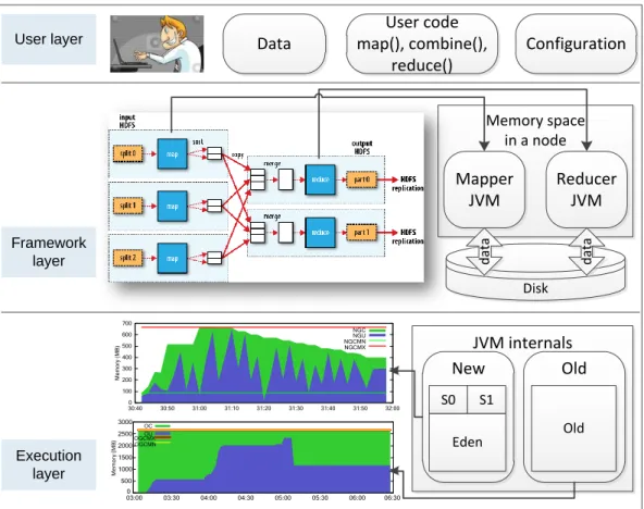
To achieve flexibility and isolation, Hadoop MapReduce consists of three system layers shown inFigure 1.1. However, this complex architecture will aggravate user’s difficulty in understanding and optimizing job’s performance, especially the memory consumption. In user layer, before submitting the job, users are required to prepare the dataset, write user code and specify appropriate configurations. In framework
layer, each job is divided into several smallmapandreducetasks. After that, each task will be scheduled onto an appropriate node. Inexecutionlayer, the node will launch each task as a separate process (i.e., a JVM instance, JVM reuse is an exception). Then, each task will perform the relatively fixed processing steps which are pre-defined by the framework.
Since JVM divides the heap space into two generations and manages them separately, execution layer is the only one that knows the real fine-grained memory usage. The blue-green graph inFigure 1.1shows the realtime usage inNewandOldgenerations of a JVM instance. Framework just treats memory as a large continuous space and has little idea of the real usage. The memory space is intensively used for both data storage (e.g., storing intermediate data) and data processing (e.g.,map() reads and processes the input data). At the highest layer, users usually feel hard to understand job’s memory usage, not to mention optimizing the usage in the large space of configurations. However, new resource management and scheduling frameworks such as YARN [6] and Mesos [8] not only require users to specify the maximum memory consumption but also schedule tasks according to the consumption. Inappropriate configurations may lead to job’s runtime error, performance degradation or the waste of memory.
Memory space in a node Data User code map(), combine(), reduce() Configuration Mapper JVM Disk Reducer JVM JVM internals New Old S0 S1 Eden Old d at a d at a User layer Framework layer Execution layer
Figure 1.1: System layers of Hadoop MapReduce
1.2 MapReduce Dataflow
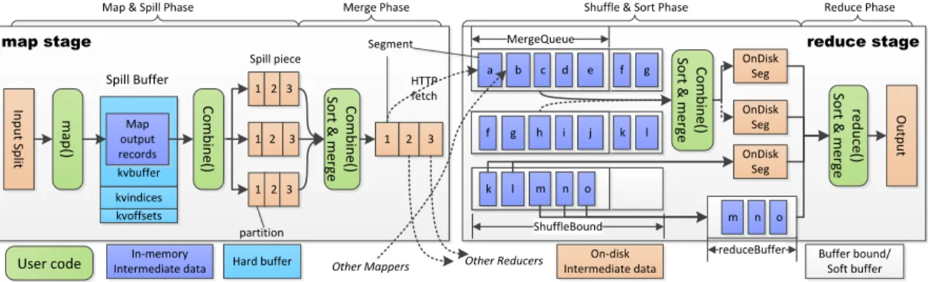
Dataflow contains two meanings: data processing steps and input/output/intermediate data in each step. The processing steps are relatively fixed, and we can merge them into four phases (shown inFigure 1.2). However, the size of input/output/intermediate data is more variable because there are many influencing factors: 1) I/O ratio of the user code. User code containsmap(),reduce() and optionalcombine(). 2) Dataflow-related configurations. 3) Data properties which may cause data skew (e.g., some reducers will need to process far more data than others). Below are the details about the processing steps and dataflow-related configurations.
Map Stage: Mapper first fetches input split (typically 64MB) from HDFS, reads sequentialhk1,v1irecords from this split, performs map() on each record and then outputshk2,v2iwith partition id into in-memory spillBuffer. Partition id is usually produced by hash or range partition function onk2. Spill buffer
consists of three arrays:kvbufferis a large byte[] that stores the serializedhk2,v2irecords. Each record is referenced by a tuple hpartition id ofk2, pointer to k2, pointer to v2iinkvindices (int[]). Each
tu-ple is referenced by a pointer inkvoffsets (int[]), so the size of kvoffsets is one third of that of
kvindices. Users can specify the size of these three arrays. Once the total size of records in spill buffer achieves a bound, mapper will sort the cachedhk2,v2irecords byk2 (only pointers in kvoffsets are sorted),
perform combine() if any on them to generate newhk2,v2irecords, and spill each piece onto the local file
reduce stage map stage map() 1 2 3 1 2 3 1 2 3 a b c d e OnDiskSeg OnDisk Seg reduce() Sort
& merge Output
1 2 3
partition
Segment
Spill Buffer
Other Mappers Other Reducers
Map & Spill Phase Merge Phase Shuffle & Sort Phase Reduce Phase
Spill piece f g m n k l OnDisk Seg MergeQueue ShuffleBound
Input Split Combine
() Combine () Sort & merge kvbuffer Combine () Sort & merge h i j k l f g m n reduceBuffer o o
User code Intermediate dataIn-memory
On-disk Intermediate data Buffer bound/ Soft buffer HTTP fetch kvindices kvoffsets Map output records Hard buffer
Figure 1.2: MapReduce dataflow in Hadoop
hk2,v2iand more than one spill piece are generated, merge phase will start. Partitions with the same id will be merged together into onesegment. Combine() may be invoked in this merge process if necessary. In the future, each segment will be fetched by one reducer according to the partition id.
Reduce Stage: Once some mappers finish (the concrete number is configurable), reducers will start and then go through three phases (shuffle, sort and reduce). In shuffle phase, reducer fetches the correspond-ing segments from finished mappers via HTTP. The fetched segments are first stored in memory. Once their total size achievesMergeQueue, the segments will be sorted, combine()ed and merged onto disk as
OnDiskSeg. Since records in each segment are ordered, this merge calledInMemShufMerge can be
performed just using a minimum heap. While merging, reducer can still fetch segments into memory until the total size of in-memory segments achievesshuffleBound. This merge action will happen many times if the total size of shuffled segments is much larger thanMergeQueue. After each merge action finishes, the merged segments will be cleared from memory. If a segment is too large, it will be fetched onto disk directly.Figure 1.2shows there are two waves ofInMemShufMergeand two segments (fandg) are left to be merged in the second wave. After all the segments are fetched from mappers, shuffle phase ends with msegments in memory andnOnDiskSegs (m,n≥0).
In the next sort phase, some ([0,m]) of themsegments will be merged to be an OnDiskSeg. The others are still cached in memory inreduceBuffer. If reduceBufferis set to 0, all themsegments will be merged onto disk. We call this mergeInMemSortMerge. After that, reducer just merges the left in-memory segments and OnDiskSegs into a logical large segment which consists ofhk2,list(v2)irecords. We
call this mergeMixSortMerge, but the actual merge action does not happen in this phase. In other words, eachhk2,list(v2)i record is not generated untilreduce() tries to read it. In reduce phase, reducer reads
thehk2,list(v2)irecords one by one, performs reduce() on each record and outputs the finalhk3,v3irecords
onto HDFS. There are some other dataflow-related configurations such as spilling threshold of spill buffer, reducer number and compress. Some of them will be introduced in the memory usage model.
1.3 JVM Memory Structure and GC
Each Java process will launch a JVM instance which isolates the program from memory management. Object allocation and garbage collection (GC) are controlled by specific algorithms. Based on theweak generational hypothesis [4] (i.e., most objects have a short survival time), JVM divides the whole heap space into new (young) and old (tenured) generations for storing objects with different survival time.
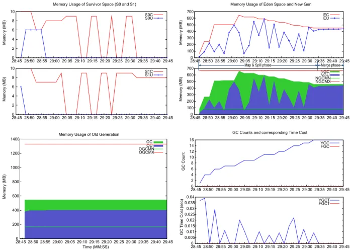
New Generation: This generation consists of one large space called Eden and two small equal-sized spaces calledSurvivor(S0 and S1). Most newly generated objects are first put into eden. When eden is nearly full, young GC (also called minor GC) occurs and some long-lived objects are transferred into one of the survivor spaces. The other space is always empty for swapping. If the long-lived objects cannot be held in the survivor space, they will be transferred intoOldgeneration. The ratio of eden to survivor can be changed at runtime by GC algorithm. Maximum size of new generation (NGCMX) is fixed by default once JVM starts.Figure 1.3shows realtime committed (C) & used (U) memory in each generation, while a WordCount mapper is running. More descriptions of the labels can be found at [5].
Memory Usage of Survivor Space (S0 and S1)
0 2 4 6 8 10 28:45 28:50 28:55 29:00 29:05 29:10 29:15 29:20 29:25 29:30 29:35 29:40 29:45 M em or y (M B ) S0C S0U 0 2 4 6 8 10 28:45 28:50 28:55 29:00 29:05 29:10 29:15 29:20 29:25 29:30 29:35 29:40 29:45 M em or y (M B ) S1C S1U
Memory Usage of Eden Space and New Gen
0 100 200 300 400 500 600 700 28:45 28:50 28:55 29:00 29:05 29:10 29:15 29:20 29:25 29:30 29:35 29:40 29:45 M em or y (M B ) EC EU 0 100 200 300 400 500 600 700 28:45 28:50 28:55 29:00 29:05 29:10 29:15 29:20 29:25 29:30 29:35 29:40 29:45 M em or y (M B ) NGC NGU NGCMN NGCMX Map & Spill phase Merge phase
0 200 400 600 800 1000 1200 1400 28:45 28:50 28:55 29:00 29:05 29:10 29:15 29:20 29:25 29:30 29:35 29:40 29:45 M em or y (M B ) Time (MM:SS) OU OGCMN OGCMX Memory Usage of Old Generation
OC
GC Counts and corresponding Time Cost
0 2 4 6 8 10 12 14 16 28:45 28:50 28:55 29:00 29:05 29:10 29:15 29:20 29:25 29:30 29:35 29:40 29:45 G C C ou nt YGC FGC 0 0.005 0.01 0.015 0.02 0.025 0.03 0.035 0.04 28:45 28:50 28:55 29:00 29:05 29:10 29:15 29:20 29:25 29:30 29:35 29:40 29:45 G C T im e C os t ( se c) YGCT FGCT
Figure 1.3: Realtime Committed & Used & GC status in each generation of a mapper
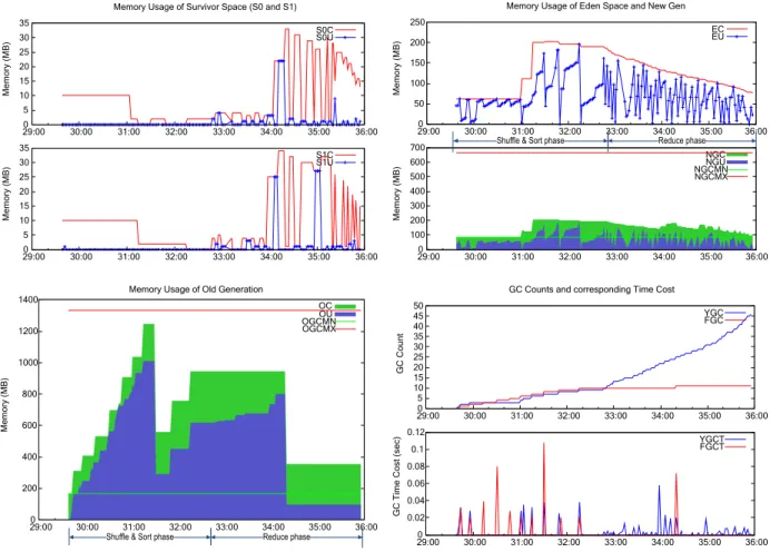
Old Generation: This space is usually larger than new generation for storing long-lived objects. Large objects such as big byte array are directly allocated in old space too. Long-lived objects in eden or sur-vivor space may retire to old space when young GC or full GC occurs. Not enough old space for storing incoming objects triggers full GC. Full GC needs to scan all the live objects in each generation and reclaim unreferenced ones. So it isheavyand time-consuming. Maximum size of old space (OGCMX) is also fixed once JVM starts, if no special configurations are specified. For mappers, spill buffer usually exists in this space. For reducers, some segments usually live in this space.Figure 1.4shows realtime committed & used memory in each generation while a reducer is running.
Memory Usage of Survivor Space (S0 and S1) 0 5 10 15 20 25 30 35 29:00 30:00 31:00 32:00 33:00 34:00 35:00 36:00 M em or y (M B ) S0C S0U 0 5 10 15 20 25 30 35 29:00 30:00 31:00 32:00 33:00 34:00 35:00 36:00 M em or y (M B ) S1C S1U
Memory Usage of Eden Space and New Gen
0 50 100 150 200 250 29:00 30:00 31:00 32:00 33:00 34:00 35:00 36:00 M em or y (M B ) EC EU 0 100 200 300 400 500 600 700 29:00 30:00 31:00 32:00 33:00 34:00 35:00 36:00 M em or y (M B ) NGC NGU NGCMN NGCMX Shuffle & Sort phase Reduce phase
0 200 400 600 800 1000 1200 1400 29:00 30:00 31:00 32:00 33:00 34:00 35:00 36:00 M em or y (M B ) OU OGCMN OGCMX Memory Usage of Old Generation
OC
Shuffle & Sort phase Reduce phase
GC Counts and corresponding Time Cost
0 5 10 15 20 25 30 35 40 45 50 29:00 30:00 31:00 32:00 33:00 34:00 35:00 36:00 G C C ou nt YGC FGC 0 0.02 0.04 0.06 0.08 0.1 0.12 29:00 30:00 31:00 32:00 33:00 34:00 35:00 36:00 G C T im e C os t ( se c) YGCT FGCT
Figure 1.4: Realtime Committed & Used & GC status in each generation of a reducer
Permanent Generation: This generation (typically 64MB) is regarded as an independent space outside heap. JVM’s reflective data such asClassandMethodobjects are stored in this space. For map/reduce tasks, the usage of this space is usually stable because tasks run the same map/reduce function. More details about this generation can be find at [4].
Memory Usage: Hadoop launches each task as a standard JVM instance, so parameters such as -Xmx
and-Xmsare also applicable to map/reduce tasks. Once Xmx is specified, maximum size of heap is fixed. The upper bound of each generation is also fixed if no special parameters are set. Some parameters can specify the ratio of new generation to old generation or survivor space to eden space. Minimum size of the heap (also as initial committed size) is determined by Xms. FormulaUsed<Committed<Maxdenotes the relationship among these three memory usage. Usedmemory is the total size of currently live objects.
Committedmemory represents the currently usable size. This size may grow or shrink according to the current ratio ofUsedtoMax. Maxmemory usually equals Xmx except that the physical memory cannot guarantee the size of Xmx.
GC Collectors: JVM contains many different garbage collectors [1] for achieving different performance goals. They can be classified into three types: Serial Collector only starts one thread to perform GC.
Parallel Collector uses multi-threads, so it is suitable for multiprocessor and applications which process large dataset. It is also the default collector of server-mode JVM. The last one isConcurrent Collector which aims at decreasing GC pauses and runs the collecting thread in parallel with the application thread. If the application runs on multiprocessor and has large set of long-lived objects, this collector is a good choice. The concrete collectors are summarized as follows. The first three collectors work in new generation and the next three ones work in old generation. G1 is a special collector which blurs the boundary of generations.
Table 1.1: Different GC collectors used in Hotspot JVM
Collectors Threads GC algorithm Other info
Serial Single Copy Default GC for client JVM
ParNew Multiple Copy Parallel version of Serial
Parallel Scavenge (PS) Multiple Copy Higher throughput
Serial Old Single Mark-Compact Can work with all
CMS Multiple Mark-Sweep Less pause time
Parallel Old Multiple Mark-Compact Can work with PS
G1 Multiple Mark-Compact+Copy Independent
There are two important issues that we need to make clear before building the memory usage model: Object location: The Hotspot GC algorithms only guarantee a single object exists in a particular gener-ation, but an object graph may span multiple generations. For example, a byte array like kvbufferis a single object, so it cannot span new and old generation. Another example isArrayList<Segment>
which contains theArrayListobject itself, theObject[]object, and the references of Segment. So theArrayListobject, the object array, and the referenced objects each will not span generations. How-ever, differentSegmentobjects can exist in different generations.
The boundary between new and old generation: The maximum heap size is fixed at JVM initialization. By default the maximum size of old generation is also fixed at initialization. There are exceptions when special configuration (e.g., UseParallelGC, UseParallelOldGC or UseG1GC) is specified. The differences between the first two collectors are as follows:
Configuration GC in new gen GC in old gen Other info
UseParallelGC Parallel Scavenge Serial Old Default GC of server-mode JVM UseParallelOldGC Parallel Scavenge Parallel Old
With UseParallelGC is specified andUseAdaptiveGCBoundary is turned on (it is on by default), the GC algorithm can move space between new generation and old generation. However, a minimum size of the new generation and a minimum size of old generation have to be observed [2]. In my practice, I have not noticed any movement between new and old generations while the map/reduce tasks are running.
If UseG1GCis specified, JVM will use G1 (Garbage-First) collector which has a new memory
man-agement mechanism. A single large contiguous Java heap space is divided into multiple fixed-sized heap regions. The new generation is a logical collection of non-contiguous regions and the collection changes dynamically. Again, the maximum size of the heap does not increase and there are limits on the minimum size of the new generation. More details can be found at [3]. Since G1 is still experimental in latest JDK 7,
we focus on the default GC collectors of server-mode JVM (i.e., there are fixed boundary between new and old generation).
2
Memory Usage Model
Last section talks a lot about the details of Hadoop and JVM internals. This section will concentrate on how to build the memory model. More formally, given a jobhdataset d, user codeuc and configurationci, we want to figure out the fine-grained memory usage of mappers and reducers.
Memory usage= f(dataset d, user code uc, configuration c) More specially, we care about two concrete memory usages in each phase.
peak usage= max t∈phase p
X
size live objectt
resident usage= max t∈phase p
X
size referenced objectt
objectt represents a live object at time t in phase p. Live objects consist of referenced objects and unreferenced objects (can be reclaimed but have not been reclaimed right now) .
Peak usage: the maximumUsedmemory. It reflects at most how much physical memory can be con-sumed by currently live objects. For example, inFigure 1.3 in map&spill phase, the peak usage of new generation is 600MB, but many objects have become unreferenced at that time. In Figure 1.4 in shuf-fle&sort phase, the peak usage of old generation is 1000MB. Peak usage can help us judge whether JVM configurations (e.g., maximum heap size) are reasonable.
Resident usage: the maximum size of all the currently referenced objects. After removing unreferenced objects, peak usage is resident usage. It reflects the minimum heap space that we should guarantee. Or else, JVM may run out of memory. For example, inFigure 1.3in map&spill phase, the usage in new generation can drop down below 100MB if the unreferenced objects are reclaimed by GC. InFigure 1.4in shuffle&sort phase, the resident usage of old generation can be lower than 1000MB because some objects may have already become unreferenced.
To model the two usages, we need to solve three questions: 1) What are in-memory objects? 2) How to calculate their sizes? 3) What is the relationship between in-memory objects and the two usages?
2.1 In-memory objects
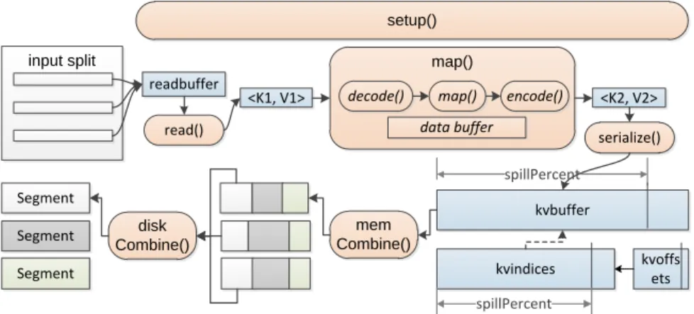
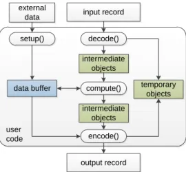
We classify in-memory objects into two types: userobjects andframeworkobjects. User objects are gen-erated by user-defined methods such as setup(), map(), combine() and reduce(). The method setup() can be invoked to do some preparation (e.g., read a dictionary into in-memory HashMap) before map()/reduce() performs on each input record. Framework objects are generated by framework for serving user code, including data buffers and in-memory intermediate data. Figure 2.1&Figure 2.2illustrate the detailed pro-cessing steps and in-memory objects in map & reduce stage. The orange ones represent user code and user objects, while the blue ones stand for framework objects. Figure 2.3 depicts the general processing steps and typical objects in user code.
In detail, we classify in-memory objects into the following types. Framework objects only include the first two types. For simplicity, some objects’ names are different with the original ones in Hadoop source code.
spillPercent input split setup() readbuffer <K1, V1> <K2, V2> map() data buffer read()
decode() map() encode()
kvbuffer kvindices kvoffs ets mem Combine() disk Combine() serialize() Segment Segment Segment spillPercent
Figure 2.1: User and framework objects in map stage
OnDiskSeg memCombine() MergeQueue ShuffleBound OnDiskSeg OnDiskSeg sortMerge reduce() data buffer
decode() reduce() encode() <K3, V3>
SortMergeQueue
<K2, list(V2)> Output
Shuffled
Segment After shuffle phase
After multi-merge Segment pointer left Segments in reduceBuffer ShuffleQueue
Figure 2.2: User and framework objects in reduce stage
Data buffers: In map stage, mapper first reads a piece of raw data from input split into a tinyreadbuffer, then it uses read() to convert the buffered data into hk1,v1i records one by one. This process is per-formed repeatedly and readbuffer is reusable. Spill buffer (i.e., kvbuffer, kvindices and kvoffsets) occupies a large fixed space for caching serialized map output records. Increasing this space may reduce spill times and disk I/O. In reduce stage, shuffled segments are first stored in logical buffers (MergeQueue
&ShuffleBound). After shuffle phase finishes, the unmerged segments are cached inreduceBuffer.
SortMergeQueuestores the pointers of all the in-memory and on-disk segments, sohk2,list(v2)irecords
can be generated one by one by merging the referenced segments. In user code, users may also allocate data buffers such as byte array, ArrayList, HashMap and other in-memory data structures. These buffers are used to keep intermediate computing results or external data. In addition, input/output/flush/compress streams may contain small-sized buffers like readbuffer.
Records: Records has two types: the input/output records of user code and the records stored in in-memory segments. User code has three features: independent,arbitraryandstreaming-style. Independent
user code input record intermediate objects temporary objects compute() data buffer encode() decode() output record external data setup() intermediate objects
Figure 2.3: General processing steps and user objects in user code
means user code only interacts with framework through records I/O. Each user code also has its own life cycle (shown inFigure 2.4), so objects generated in current user code will become useless when the next user code is invoked by the framework. For example, objects used in map() will not be available in combine(). Arbitrarymeans there is no constraint on user code except the input/output format, so any objects may be defined and generated in user code.Streaming-stylemeans records are read, processed and outputted one by one. So current input record and its associative intermediate computing results may become unreferenced when the next record is read in. The records stored in-memory segments are framework objects, because they are managed by framework.
Intermediate objects: There are also two types of intermediate objects in user code. One is the record-related objects that are generated by type conversion. Since input/output records are serialized objects (extends Writable), it is not convenient to process them directly. In general, method decode() is used to convert input records to ordinary Java objects, while encode() does the reverse job. So the number and size of these record-related objects always have linear correlation with the input/output records. The other type is the intermediate processing results that are generated during the concrete computation. For example, the words tokenized from the input string are regarded as intermediate objects in WordCount mapper. Most intermediate objects are useless while the next record is going to be processed, but some of them may be kept in data buffer for further use. For example, de-duplication will allocate a HashSetto cache each unique intermediate object generated from current input record.
Temporary objects: While performing decode() and encode() on each record, temporarily referenced ob-jects such as char[], byte[], String and so on may be generated accordingly. These obob-jects are different from intermediate objects because temporary objects are useless once the type conversion is over. For example, A WordCount mapper produces massivejava.nio.HeapCharBufferobjects while encoding the to-kenizedStringobjects toTextobjects. The number of HeapCharBuffer objects is as same as the output records of map() and their total size is more than 7 times of the input split (shown in TableTable 2.1).
Other objects: Apart from the framework, other components in Hadoop such as the scheduler, monitor, and task tracker may generate some small objects while tasks are running. We regard these objects as other objects but not consider them in the memory usage model.
To give a detailed example, we collect the top memory-consuming objects while WordCount mapper and reducer are running.
Table 2.1: Dataflow counters and top memory-consuming objects in a WordCount mapper
Abbreviation Dataflow counters Value
mapInRecs Map input records 3,964
mapOutRecs Map output records 10,486,900 combineInRecs Combine input records 12,114,758 combineOutRecs Combine output records 2,342,038
bytes number of objs object names generated by 503,371,200 10,486,900 java.nio.HeapCharBuffer encode() 503,371,200 10,486,900 java.nio.HeapByteBuffer encode()
335,580,800 10,486,900 java.lang.String intermediate objects
310,333,240 10,486,900 char[] encode()
264,945,096 10,486,900 byte[] encode()
199,229,456 1 byte[] kvbuffer
150,953,328 18,391 byte[] input stream buffer
134,309,656 3,964 char[] decode()
133,835,536 3,964 char[] decode()
7,864,336 1 int[] kvindices
5,660,592 117,929 java.nio.HeapByteBuffer encode()
3,733,872 1,010 byte[] other object
2,621,456 1 int[] kvoffsets
2,566,272 26,732 int[] other object
2,206,920 18,391 int[] other object
2,158,704 263 byte[] input stream buffer
1,800,264 31 byte[] enlarged readbuffer
1,733,760 54,180 java.util.HashMap$Entry other object
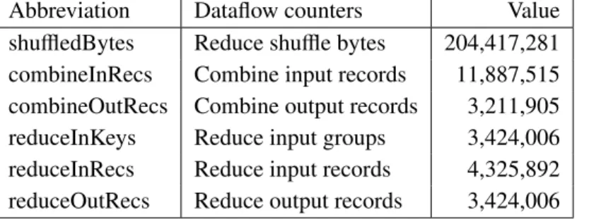
Table 2.2: Dataflow counters and top memory-consuming objects in a WordCount reducer
Abbreviation Dataflow counters Value
shuffledBytes Reduce shuffle bytes 204,417,281 combineInRecs Combine input records 11,887,515 combineOutRecs Combine output records 3,211,905 reduceInKeys Reduce input groups 3,424,006 reduceInRecs Reduce input records 4,325,892 reduceOutRecs Reduce output records 3,424,006
bytes number of objs object names generated by 164,352,288 3,424,006 java.nio.HeapByteBuffer encode() 164,352,288 3,424,006 java.nio.HeapCharBuffer encode()
140,611,248 17,131 byte[] input stream buffer
109,568,192 3,424,006 java.lang.String intermediate objects
82,559,704 3,424,006 byte[] encode()
82,187,840 3,424,006 char[] encode()
82,176,144 3,424,006 byte[] intermediate objects
43,765,272 32 byte[] Segments/Records
43,728,480 32 byte[] Segments/Records
39,647,648 29 byte[] Segments/Records
39,304,792 29 byte[] Segments/Records
37,973,432 28 byte[] Segments/Records
37,378,320 570 byte[] write stream buffer
10,426,584 159 byte[] write stream buffer
2.2 Life cycle
The life cycles of objects are important to determine the peak and resident usage.
Type Abbreviation Concrete type Life cycle
Framework data buffer phase
records buffer
User code tObj temporary objects record
intermediate objects record
rObj data buffer user code
Framework objects: Data buffer isphaselevel, since it will exist in memory from the beginning to the end of the phase. Records arebufferlevel because records are first stored in the buffer and will be merged onto the disk when the buffer is nearly full.
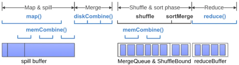
User objects have two types: tObjs represents temporarily referenced objects, while rObjs stands for resident objects. tObjs arerecord level and consist of two subtypes. Temporary objects can be reclaimed once the corresponding record finishes type conversion. Intermediate objects can be reclaimed once the next record is read in, except that they are kept in long-lived data buffer.rObjsareuser codelevel, because necessary intermediate objects or external data will be kept in the data buffer until the user code ends.
To detail the user code level,Figure 2.4shows the concrete life cycle of each user code. Although setup() actually runs before map(), therObjsin it can exist in memory until map() finishes. Each combine() is in-dependent, sorObjswhich exist in current memCombine() can be reclaimed when the next memCombine() is invoked.
Map & spill Merge Shuffle & sort phase Reduce
spill buffer MergeQueue & ShuffleBound reduceBuffer
shuffle
map() diskCombine()
memCombine() memCombine()
reduce() sortMerge
Figure 2.4: The life cycles of user code and framework objects
2.3 Size calculation
Suppose we have known the dataflow counters (i.e., the data size in each processing step), we can model the size of in-memory objects in different phases.
Size(objects)= f(dataflow d, user code uc, configuration c)
Some framework objects likekvbufferare only related to the configuration, while others likeSegment
is affected by both the dataflow counters and configurations.
User objects are hard to estimate before the job runs. We do not know whether users will define data buffer and how many intermediate data will be kept in the buffer. We also do not know the size oftObjs. But fromTable 2.1andTable 2.2, we can see that there is a linear relationship betweentObjsand input/output records. So, if the job has run before, we can profile the buffer size and estimate the ratio of tObjs to input/output records using linear regression.
The following tables reflect the concrete f() in each phase. Configurations are marked with blue. U is user objects, while F is framework objects. tObj(counter) denotes the size of total tObjsis affected by the counter.rObj(method) stands for the size of resident objects in that method. Some counters likemapInRecs will be detailed in the next section.
After computing the size and life cycles of in-memory objects, we can model the peak and resident usage. The peak usage model assumes all the in-memory objects are not reclaimed in the current phase, while resident usage model does not consider unreferenced objects.
Setup phase
Objects Type U or F Total size setup() Data buffer U rObj(setup) Map&Spill phase
Objects Type U or F Total size
kvbuffer Data buffer F io.sort.mb* (1 -io.sort.record.percent) kvoffsets Data buffer F io.sort.mb*io.sort.record.percent/4 kvindices Data buffer F 3 * kvoffsets
map() Data buffer U tObj(mapInRecs)+tObj(mapOutRecs)+rObj(map) tObjs
memCombine() Data buffer U PSpillTimes
i=1 {tObj(memCombineInRecsi)
tObjs +tObj(memCombineOutRecsi)
total(map)=kvbuffer+kvindices+kvoffsets+map()+memCombine() peak usage=min(total(map),maxHeapSize)
resident usage=kvbuffer+kvindices+kvoffsets+rObj(map)+ max
1≤i≤SpillTimes(rObj(memCombinei)) Merge phase
Objects Type U or F Total size
diskCombine() Data buffer U PReduceNum
i=1 {tObj(diskCombineInRecsi)
tObjs +tObj(diskCombineOutRecsi) +rObj(diskCombinei)}
peak usage=min(total(map)+diskCombine(),maxHeapSize) resident usage=max(rObj(diskCombinei))
If the objects in map & spill phase have been reclaimed before merge phase, the peak usage of merge phase will decrease.
Shuffle&Sort phase
Objects Type U or F Total size
Segment Records F shuffledSegments
(Total shuffled)
Segment Records F min(shuffledSegments,MergeQueue) (MergeQueue)
Segment Records F min(shuffleBound,shuffledSegments)−MergeQueue (ShuffleQueue) or 0 (if shuffledSegments<MergeQueue)
memCombine() Data buffer U PMergeTimes
i=1 {tObj(memCombineInRecsi)
tObjs +tObj(memCombineOutRecsi)
+rObj(memCombinei)}
The first segment denotes the total shuffled segments in a reducer. The second one represents the max-imum size of segments in MergeQueue. The third one stands for the maxmax-imum size of segments in shuffl e-Bound but not in MergeQueue.
shuffleSegments=uncompressed(reduce shuffle bytes)
shuffleBound=maxHeapSize∗mapred.job.shuffle.input.buffer.percent MergeQueue=shuffleBound∗mapred.job.shuffle.merge.percent total(shuffle&sort)=shuffledSegments+memCombine()
peak usage=min(total(shuffle&sort),maxHeapSize)
resident usage=min(shuffledSegments,shuffleBound)+ max
Reduce phase
Objects Type U or F Total size
Segment Records F min(reduceBuffer,shuffledSegements%MergeQueue) (reduceBuffer)
reduce() Data buffer U tObj(reduceInRecs)+tObj(reduceOutRecs)
tObjs +rObj(reduce)
By default, reduceBuffer (mapred.job.reduce.input.buffer.percent) is set to 0, so all the segments have been merged onto disk before reduce phase starts.
total(reduce)=Segment(reduceBuffer)+reduce()
peak usage=min(total(shuffle&sort)+total(reduce),maxHeapSize) resident usage=Segment(reduceBuffer)+rObj(reduce)
After a job finishes, the driver program, which is originally used to submit the job, can also be used to collect the outputs of reducers. This collector is common in iterative jobs like Mahout jobs, but not every job has it.
Collect phase
Objects Type U or F Total size
Collect() Data buffer U tObj(reduceOutRecs)+rObj(collect) tObjs
peak usage=min(tObj(reduceOutRecs)+rObj(collect),maxHeapSize) resident usage=rObj(collect)
2.4 Dataflow model
As seen from above, size of in-memory objects is closely related to dataflow counters. So we need to have a dataflow model. Many materials such as [7] have invented this wheel. Here, we give a simplified version which focuses on the memory-related dataflow counters. Some formulas assume there is no data skew. Notations
r(methodInRecs) represents the output records of the method, given the input records. bprdenotes the bytes per record in current counter.
bpris different in different counters, but we use the same notation in each counter for simplicity. r(memCombine)=r(diskCombine)=1, if there is no combine() in the job.
Recsis the abbreviation of records. Map stage
Counters Calculation
mapInRecs InputSplit/bpr
mapOutRecs mapInRecs∗r(mapInRecs) memCombineInRecs PSpillTimes i=1 (memCombineInRecsi) memCombineOutRecs PSpillTimes i=1 (r(memCombineInRecsi)) diskCombineInRecs PReduceNum i=1 (diskCombineInRecsi) diskCombineOutRecs PReduceNum i=1 (r(diskCombineInRecsi)) spillPercent=io.sort.spill.percent
spillRecords=min kvbuffer∗spillPercent
bpr ,
kvoffsets∗spillPercent
4 ,mapOutRecs ! SpillTimes= & mapOutRecs spillRecords '
memCombineInRecsi =spillRecords, (i f1≤i<spillTimes)
memCombineInRecsi =mapOutRecs%spillRecords, (i f i=SpillTimes) diskCombineInRecsi =
memCombineOutRecs
ReduceNum
Reduce stage
Counters Calculation
shuffledSegments PMapperNum
i=1 (diskCombineOutRecs∗bpr/reduceNum)
memCombineInRecs PMergeTimes
i=1 (memCombineInRecsi)
memCombineOutRecs PMergeTimes
i=1 (r(memCombineInRecsi))
reduceInRecs memCombineOutRecs+(shuffledSegments%MergeQueue)/bpr reduceOutRecs r(reduceInRecs) MergeTimes= $ shuffledSegments MergeQueue % memCombineInRecsi = min(P
(unmerged segment),MergeQueue) bpr
2.5 Peak&resident usage in each generation
Until now, we have calculated the peak and resident memory usage in mapper/reducer. If we want to delve into the memory usage in each generation, the following will help.
In this section, we will model the peak usage in each generation by analyzing the object locations and GC’s effects. We first map the in-memory objects into each generation. Then, we will discuss how the GC affects the peak usage. A general model is summarized based on the memory management mechanism of JVM and the life cycles of in-memory objects.
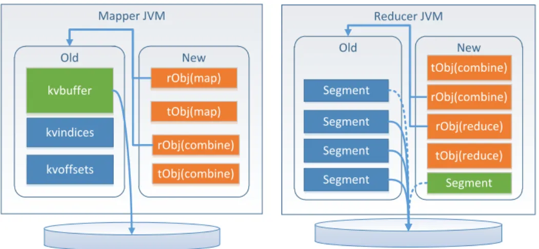
Mapper JVM Old New kvbuffer kvindices kvoffsets rObj(map) Reducer JVM Old New tObj(combine) Segment Segment Segment Segment tObj(map) rObj(combine) tObj(combine) rObj(combine) rObj(reduce) tObj(reduce) Segment
Figure 2.5: General JVM model of mappers and reducers
Object locations
The location rules are applicable to most jobs but not all the jobs. JVM will put large objects and old enough objects into old gen (abbr. of generation). Temporarily referenced objects are mainly allocated and reclaimed in new gen. There are also exceptions: when old gen is full, some long-lived objects will still exist in new gen (e.g., the green segment in MergeQueue or shuffleBound). Resident objects are easy to retire to old gen if the new gen is too small.
Mapper JVM Since spillBuffer is large enough and exists in memory for a long time, it is assumed to be in the old gen. tObjsgenerated in map() and combine() are only referenced while the corresponding record is being processed. As a result, fewtObjsare transferred to old gen. rObjsare assumed to be first allocated in new gen, then some of them may retire to old gen. For example, map() allocates an ArrayList to keep all the decoded input records. Some early added records may retire to old gen, while others may still exist in new gen. However, if the ArrayList is substituted by a large byte buffer, the buffer will exist in old gen as same as spill buffer.
Figure 1.3shows the realtime usage of a mapper JVM every 2 seconds. After a minor GC, mosttObjs are reclaimed and the usage drops down dramatically. The usage of old gen is stable because only spill buffer exists in it.
Reducer JVM In shuffle & sort phase, shuffled segments are first fetched into the new gen. When new gen is nearly full, minor GC will occur. Some segments will retire to old gen since different segments can exist in different generations as mentioned insection 1.3. Segments in MergeQueue are easier to be transferred to old gen because time-consuming merge will make them long-lived. Other segments in MergeQueue may still exist in new gen because old gen may have not enough space. After segments are merged onto disk, they become unreferenced and will be reclaimed if full GC occurs. Segments in shufflebound but not in MergeQueue are relatively fresh, so they may exist in new gen except that new gen is full. In reduce phase, the left segments in reducebuffer are supposed to be in old gen because they are old enough. The locations oftObjsandrObjsare as same as them in map().
Note that the following models are general but not absolute. For example, some objects in the new gen may retire to old gen at run time.
Peak usage
Phase New Old
Map & spill map()+memCombine() spillBuffer
Merge diskCombine()
Shuffle & sort shuffledSegments+memCombine() Segments(MergeQueue)
Reduce reduce() Segments(reduceBuffer)
Resident usage
Phase New Old
Map & spill rObj(MapInRecs)+max(rObj(memCombinei)) spillBuffer
Merge max(rObj(diskCombinei))
Shuffle & sort Segment(shuffleQueue)+max(rObj(memCombinei)) Segment(MergeQueue)
Reduce rObj(ReduceInRecs) Segments(reduceBuffer)
References
[1] https://blogs.oracle.com/jonthecollector/entry/our_collectors.
[2] http://mail.openjdk.java.net/pipermail/hotspot-gc-dev/2013-August/008135.html. [3] http://www.infoq.com/articles/G1-One-Garbage-Collector-To-Rule-Them-All.
[4] GC Tuning. http://www.oracle.com/technetwork/java/javase/gc-tuning-6-140523.html. [5] Jstat. http://docs.oracle.com/javase/6/docs/technotes/tools/share/jstat.html.
[6] YARN. http://hadoop.apache.org/docs/current/hadoop-yarn/hadoop-yarn-site/YARN.html. [7] H. Herodotou. Hadoop performance models. CoRR, abs/1106.0940, 2011.