Journal of Financial Economics

Corporate bond liquidity before and after the onset of the

subprime crisis

$

Jens Dick-Nielsen

a

, Peter Feldh ¨utter

b

, David Lando

a,n

a

Department of Finance, Copenhagen Business School, Solbjerg Plads 3, DK-2000 Frederiksberg, Denmark b

London Business School, Regent’s Park, London NW1 4SA, United Kingdom

a r t i c l e

i n f o

Article history: Received 6 July 2010 Received in revised form 9 May 2011

Accepted 28 May 2011

Available online 3 November 2011 JEL classification: C23 G01 G12 Keywords: Corporate bonds Liquidity Liquidity risk Subprime crisis

a b s t r a c t

We analyze liquidity components of corporate bond spreads during 2005–2009 using a new robust illiquidity measure. The spread contribution from illiquidity increases dramatically with the onset of the subprime crisis. The increase is slow and persistent for investment grade bonds while the effect is stronger but more short-lived for speculative grade bonds. Bonds become less liquid when financial distress hits a lead underwriter and the liquidity of bonds issued by financial firms dries up under crises. During the subprime crisis, flight-to-quality is confined to AAA-rated bonds.

&_{2011 Elsevier B.V. All rights reserved.}

1. Introduction

The onset of the subprime crisis caused a dramatic widening of corporate bond spreads. In light of the strong

evidence that illiquidity in addition to credit risk con-tributes to corporate bond spreads, it is reasonable to believe that at least part of the spread-widening can be attributed to a decrease in bond liquidity. We use TRACE (Trade Reporting and Compliance Engine) transactions data for corporate bonds and a new measure of liquidity to analyze how illiquidity has contributed to bond spreads before and after the onset of the subprime crisis. Our liquidity measure outperforms the Roll (1984) measure used inBao, Pan, and Wang (2011)and zero-trading days used in Chen, Lesmond, and Wei (2007) in explaining spread variation.

We use the measure to define the liquidity component of bond spreads as the difference in bond yields between a bond with average liquidity and a very liquid bond. At the onset of the crisis, the liquidity component rose for all rating classes except AAA. The increase occurred both because of falling bond liquidity and because of increased sensitivity of bond spreads to illiquidity. Before the crisis

Contents lists available atSciVerse ScienceDirect

journal homepage:www.elsevier.com/locate/jfec

Journal of Financial Economics

0304-405X/$ - see front matter&_{2011 Elsevier B.V. All rights reserved.}

doi:10.1016/j.jfineco.2011.10.009

$

We thank Yakov Amihud, Sreedhar Bharath, Jeff Bohn, Michael Brennan, Tom Engsted, Edie Hotchkiss, Loriano Mancini, Marco Pagano, Lasse Pedersen, Ilya Strebulaev and participants at seminars at the Goethe University in Frankfurt, Danmarks Nationalbank, Deutsche Bundesbank, ECB, AQR Asset Management, Moody’s Investors Service, Oesterreichische Nationalbank, CBS, NYU, PenSam, VU University Amsterdam, USI Lugano, and at conferences in Bergen (EFA), Konstanz, Florence, London (Moody’s 7th Credit Risk Conference 2011), EPFL Lausanne, and Venice for helpful comments. Peter Feldh ¨utter thanks the Danish Social Science Research Council for financial support. We are especially indebted to the referee Edith Hotchkiss for many valuable suggestions.

n

Corresponding author.

E-mail addresses:jdn.fi@cbs.dk (J. Dick-Nielsen),

the liquidity component was small for investment grade, ranging from 1 basis point (bp) for AAA to 4bp for BBB. For AAA bonds the contribution remained small at 5bp during the crisis—consistent with a flight-to-quality into those bonds. More dramatically, the liquidity component for BBB bonds increased to 93bp, and for speculative grade bonds rose from 58 to 197bp. For speculative grade bonds, premiums peaked around the Lehman Brothers default in the fall of 2008 and returned almost to pre-crisis levels in the summer of 2009.

We also use our measure to provide suggestive evidence of the mechanisms by which bond liquidity was affected. If lead underwriters are providers of liquidity of a bond in secondary market trading, it is conceivable that financial distress of a lead underwriter causes the liquidity of the bond to decrease relative to other bonds. We find that bonds which had Bear Stearns as lead underwriter had lower liquidity during the take-over of Bear Stearns and bonds with Lehman as lead underwriter had lower liquidity around the bankruptcy of Lehman. Furthermore, we inves-tigate whether the time-series variation of liquidity of corporate bonds issued by financial firms is different from the variation for bonds issued by industrial firms. Our time-series study reveals that bonds issued by financial firms had similar liquidity as bonds issued by industrial firms, except in extreme stress periods, where bonds of financial firms became very illiquid, overall and when compared to bonds issued by industrial firms. A potential explanation is the heightened information asymmetry regarding the state of financial firms.

Finally, measuring the covariation of an individual bond’s liquidity with that of the entire corporate bond market, we find that this measure of systematic liquidity risk was not a significant contributor to spreads before the onset of the crisis but did contribute to spreads after the onset except for AAA-rated bonds. This indicates that the flight-to-quality effect in investment grade bonds found inAcharya, Amihud, and Bharath (2010)is confined to AAA-rated bonds.

Our liquidity measure, which we denote

l

, is an equally weighted sum of four variables all normalized to a common scale: Amihud’s measure of price impact, a measure of roundtrip cost of trading, and the variability of each of these two measures. We can think of the Amihud measure and the roundtrip cost measure as measuring liquidity, and the variability measures as representing the sum of systematic and unsystematic liquidity risk. Due to the infrequent trading of bonds, we find it difficult to measure the systematic part accurately on a frequent basis, so we use total liquidity risk and study the systematic part separately.

l

is a close approximation to the first principal component extracted among a large number of potential liquidity proxies. When we regress corporate bond spreads on

l

and control for credit risk, the measure contributes to spreads consistently across ratings and in our two regimes. This consistency is important for drawing conclusions when we split the sample by industry and lead underwriter. The TRACE transactions data allow us to calculate liquidity proxies more accurately and help us shed new light on previous results on liquidity in corporate bonds. Once actual transactions data are used, the finding inChen, Lesmond, and Wei (2007) that zero-trading days predict spreads

largely disappears. In fact, the number of zero-trading days tends to decrease during the crisis, because trades in less liquid bonds are split into trades of smaller size.

We perform a series of robustness checks, and the two most important checks are as follows. To support the claim that our measure

l

is not measuring credit risk, we run regressions on a matched sample of corporate bonds using pairs of bonds issued by the same firm with maturity close to each other. Instead of credit controls, we use a dummy variable for each matched pair and estimate how spreads depend on

l

. In this alternative approach to controlling for credit risk,

l

consistently remains significant. The second check relates to the fact that we use data for bonds for which we have transactions for some period during 2005– 2009. To test that our results are not confounded by an increase in new issues towards the end of the sample period, we redo results using only bonds in existence by 2005, and results remain similar.

The literature on how liquidity affects asset prices is extensive. A comprehensive survey can be found in

Amihud, Mendelson, and Pedersen (2005). In recent years, the illiquidity of corporate bonds has been seen as a possible explanation for the ‘credit spread puzzle,’ i.e., the claim that yield spreads on corporate bonds are larger than what can be explained by default risk (seeHuang and Huang, 2003; Elton, Gruber, Agrawal, and Mann, 2001; Collin-Dufresne, Goldstein, and Martin, 2001). Earlier papers showing that liquidity proxies are significant explanatory variables for credit spreads are Houweling, Mentink, and Vorst (2005),Downing, Underwood, and Xing (2005),de Jong and Driessen (2006),Sarig and Warga (1989), andCovitz and Downing (2007).Lin, Wang, and Wu (2011)

study liquidity risk in the corporate bond market but do not focus on the regime-dependent nature of liquidity risk.Bao, Pan, and Wang (2011)extract an aggregate liquidity mea-sure from investment grade bonds using the Roll meamea-sure and examine the pricing implications of illiquidity. The fact that

l

is more robust than the Roll measure allows us to get a more detailed picture of bond market liquidity across underwriter, sector, and rating. Furthermore, we investigate the liquidity of both investment grade and speculative grade bonds.

2. Data description

Since January 2001, members of the Financial Industry Regulatory Authority have been required to report their secondary over-the-counter corporate bond transactions through TRACE (Trade Reporting and Compliance Engine). Because of the uncertain benefit to investors of price transparency, not all trades reported to TRACE were initially disseminated at the launch of TRACE on July 1, 2002. Since October 2004, trades in almost all bonds except some lightly traded bonds are disseminated (see

Goldstein and Hotchkiss, 2008, for details). Because we use quarterly observations, we start our sample period at the beginning of the subsequent quarter.

We use a sample of corporate bonds which have some trade reports in TRACE during the period January 1, 2005 to June 30, 2009. We limit the sample to fixed rate bullet bonds that are not callable, convertible, putable, or have

sinking fund provisions. We obtain bond information from Bloomberg, and this provides us initially with 10,785 bond issues. We use ratings from Datastream and bonds with missing ratings are excluded.1 _{This reduces the sample to}

5,376 bonds. Retail-sized trades (trades below $100,000 in volume) are discarded and after filtering out erroneous trades, as described inDick-Nielsen (2009), we are left with 8,212,990 trades. Finally, we collect analysts’ forecast dis-persion from IBES, share prices for the issuing firms and firm accounting figures from Bloomberg, swap rates from Data-stream, Treasury yields consisting of the most recently auctioned issues adjusted to constant maturities published by the Federal Reserve in the H-15 release, and LIBOR rates from British Bankers’ Association. If forecast dispersion, share prices, or firm accounting figures are not available, we drop the corresponding observations from the sample.

3. Empirical methodology

This section provides details on the regression analysis conducted in the next section and defines the set of liquidity variables we use.

3.1. Regression

As dependent variable we use the yield spread to the swap rate for every bond at the end of each quarter. Implementation details are given inAppendix A.

To control for credit risk, we followBlume, Lim, and MacKinlay (1998)and add the ratio of operating income to sales, ratio of long term debt to assets, leverage ratio, equity volatility, and four pretax interest coverage dum-mies to the regressions.2_{To capture effects of the general}

economic environment on the credit risk of firms, we include the level and slope of the swap curve, defined as the 10-year swap rate and the difference between the 10-year and 1-year swap rate. Duffie and Lando (2001)

show that credit spreads may increase when there is incomplete information on the firm’s true credit quality. To proxy for this effect, we follow G ¨untay and Hackbarth (2010)and use dispersion in earnings forecasts as a measure of incomplete information. Finally, we add bond age, time-to-maturity, and size of coupon to the regressions; see, for example,Sarig and Warga (1989),Houweling, Mentink, and Vorst (2005), andLongstaff, Mithal, and Neis (2005). We do not use Credit Default Swap (CDS) data since that would

restrict the sample to only those firms for which CDS contracts are trading.

For each rating class, we run separate regressions using quarterly observations. The regressions are Spreadit¼

a

þ

g

Liquidityitþ

b

1Bond ageit

þ

b

2Amount issueditþ

b

3Couponit þ

b

4Time-to-maturityitþ

b

5Eq:volit

þ

b

6Operatingitþ

b

7Leverageitþ

b

8Long debtit þ

b

9,pretaxPretax dummiesitþ

b

1010y Swapt þ

b

1110y21y Swapt

þ

b

12Forecast dispersionitþ

Eit

, ð1Þ whereiis bond issue,tis quarter, and Liquidityitcontains one of the liquidity proxies defined below. Since we have panel data of yield spreads with each issuer potentially having more than one bond outstanding at any point in time, we calculate two-dimensional cluster robust standard errors (see

Petersen, 2009). This corrects for time-series effects, firm fixed effects, and heteroskedasticity in the residuals.

3.2. Liquidity measures

There is no consensus on how to measure the liquidity of an asset so we examine a number of liquidity-related measures for corporate bonds.Appendix Adescribes the measures and their implementation in more detail.

We use theAmihud (2002)illiquidity measure to esti-mate theprice impact of trades, defined as the price impact of a trade per unit traded. We proxy forbid–ask spreads using two different measures, the Roll measure and Imputed Roundtrip Trades. Roll (1984) finds that under certain assumptions, the bid–ask spread can be extracted from the covariance between consecutive returns, and the Roll measure is based on this insight. Feldh ¨utter (in press)

proposes to measure bid–ask spreads using Imputed Round-trip Trades (IRT). Most of the data do not contain informa-tion about the buy and sell side in trades, and IRTs are based on finding two trades close in time that are likely to be a buy and a sell. Such trades are used to construct Imputed Roundtrip Costs, IRC, as explained inAppendix A.

We also consider trading activity measures.Turnoveris the quarterly turnover in percent of total amount out-standing, whilezero-trading daysmeasures the percentage of days during a quarter where a bond does not trade. We also calculatefirm zero-trading daysas the percentage of days during a quarter where none of the issuing firm’s bonds traded. Even if a single bond seldom trades, the issuing firm might have many bonds outstanding and there might be frequent trading in these close substitutes. Finally, we considerliquidity riskby taking the stan-dard deviation of daily observations of the Amihud measure and Imputed Roundtrip Trades. These two mea-sures do not separate total liquidity risk into a systematic and unsystematic component. Arguably, only the systematic component is important for pricing, but we find it difficult to measure this component on a frequent basis, so we calculate the total component and address the systematic component later in the paper.

Mahanti, Nashikkar, Subramanyam, Chacko, and Mallik (2008) infer a turnover measure for bonds from bond 1

We use the rating from Standard and Poor’s. If this rating is missing, we use the rating from Moody’s and if this is missing, the rating from Fitch. If we still do not have a rating we use the company rating.

2_{The pretax interest coverage dummies are defined as follows. We} define the pretax interest rate coverage (IRC) ratio as EBIT divided by interest expenses. It expresses how easily the company can cover its interest rate expenses. However, the distribution is highly skewed. As in Blume, Lim, and MacKinlay (1998), we control for this skewness by creating four dummies (pretax dummies) which allows for a non-linear relationship with the spread. The first dummy is set to the IRC ratio if it is less than 5 and 5 if it is above. The second dummy is set to zero if IRC is below 5, to the IRC ratio minus 5 if it lies between 5 and 10, and 5 if it lies above. The third dummy is set to zero if IRC is below 10, to the IRC ratio minus 10 if it lies between 10 and 20, and 10 if it lies above. The fourth dummy is set to zero if IRC is below 20 and is set to IRC minus 20 if it lies above 20 (truncating the dummy value at 80).

investors’ portfolios, called latent liquidity. We are inter-ested in yield spread effects of illiquidity, so we confine ourselves to the more liquid segment of the corporate bond market for which some prices are observed, and for this reason we do not use latent liquidity.

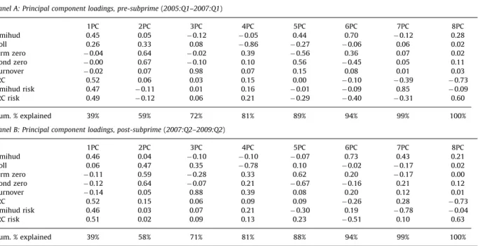
To see if most of the relevant information in the liquidity proxies can be captured by a few factors, we conduct a principal component (PC) analysis in Table 1for the two periods 2005:Q1–2007:Q1 and 2007:Q2–2009:Q2.3 _The

explanatory power and the loadings of the first four PCs are stable in the two periods and we see that they have clear interpretations. The first component explains 40% of the variation in the liquidity variables and is close to an equally weighted linear combination of the Amihud and IRC mea-sures and their associated liquidity risk meamea-sures. The second PC explains 20% and is a zero-trading days measure, the third PC explains 13% and is a turnover measure, and the fourth PC explains 9% and is a Roll measure. The last four PCs explain less than 20% and do not have clear interpretations. The principal component loadings on the first PC in

Table 1 lead us to define a factor that loads evenly on Amihud, IRC, Amihud risk, and IRC risk, and does not load on the other liquidity measures. The factor is simpler to calcu-late than the first PC while retaining its properties. We add this factor to our liquidity proxies in our analysis and call it

l

(for details, seeAppendix A).

4. Liquidity premia

4.1. Summary statistics

Table 2 shows summary statistics for the liquidity variables. We see that the median quarterly turnover is 4.5%, meaning that for the average bond in the sample, it takes five to six years to turn over once.4 _{The median}

number of bond zero-trading days is 60.7%, consistent with the notion that the corporate bond market is an illiquid market. We also see that the median number of firm zero-trading days is 0%. This shows that although a given corporate bond might not trade very often, the issuing firm typically hassomebond that is trading.

The median Amihud measure is 0.0044 implying that a trade of $300,000 in an average bond moves price by roughly 0.13%. Han and Zhou (2008) also calculate the Amihud measure for corporate bond data using TRACE data and find a much stronger price effect of a trade. For example, they find that a trade of $300,000 in a bond, on average, moves the price by 10.2%. This discrepancy is largely due to the exclusion of small trades in our sample and underscores the importance of filtering out retail trades when estimating transaction costs of institutional investors.

The median roundtrip cost in percentage of the price is 0.22% according to the IRC measure, while the roundtrip Table 1

Principal component loadings on the liquidity variables.

This table shows the principal component analysis loadings on each of the eight liquidity variables along with the cumulative explanatory power of the components. The liquidity variables are measured quarterly for each bond in the data sample. The data are U.S. corporate bond transactions data from TRACE and the sample period is from 2005:Q1 to 2009:Q2.

Panel A: Principal component loadings, pre-subprime(2005:Q1–2007:Q1)

1PC 2PC 3PC 4PC 5PC 6PC 7PC 8PC Amihud 0.45 0.05 0.12 0.05 0.44 0.70 0.12 0.28 Roll 0.26 0.33 0.08 0.86 0.27 0.06 0.06 0.02 Firm zero 0.04 0.64 0.02 0.39 0.56 0.36 0.07 0.02 Bond zero 0.00 0.67 0.10 0.10 0.56 0.45 0.05 0.11 Turnover 0.02 0.07 0.98 0.07 0.15 0.08 0.01 0.03 IRC 0.52 0.06 0.03 0.15 0.00 0.10 0.39 0.73 Amihud risk 0.47 0.11 0.01 0.16 0.01 0.09 0.85 0.09 IRC risk 0.49 0.12 0.06 0.21 0.29 0.40 0.31 0.60 Cum. % explained 39% 59% 72% 81% 89% 94% 99% 100%

Panel B: Principal component loadings, post-subprime(2007:Q2–2009:Q2)

1PC 2PC 3PC 4PC 5PC 6PC 7PC 8PC Amihud 0.46 0.04 0.10 0.10 0.07 0.73 0.43 0.21 Roll 0.06 0.47 0.35 0.78 0.10 0.02 0.17 0.02 Firm zero 0.11 0.59 0.28 0.33 0.62 0.20 0.17 0.00 Bond zero 0.12 0.64 0.07 0.21 0.67 0.16 0.21 0.12 Turnover 0.14 0.05 0.88 0.39 0.08 0.20 0.12 0.01 IRC 0.52 0.15 0.06 0.09 0.09 0.26 0.28 0.73 Amihud risk 0.46 0.03 0.07 0.21 0.30 0.19 0.78 0.04 IRC risk 0.51 0.02 0.09 0.13 0.23 0.51 0.10 0.63 Cum. % explained 39% 58% 71% 81% 88% 94% 99% 100% 3

An extensive analysis of latent common factors in liquidity measures for equity markets can be found in Korajczyk and Sadka (2008).

4

The turnover is a lower bound on the actual turnover since trade sizes above $1mil ($5mil) for speculative (investment) grade bonds are registered as trades of size $1mil ($5mil).

cost is less than 0.05% for the 5% most liquid bonds. Thus, transaction costs are modest for a large part of the corporate bond market, consistent with findings in Edwards, Harris, and Piwowar (2007),Goldstein, Hotchkiss, and Sirri (2007), andBessembinder, Maxwell, and Venkaraman (2006).

The correlations in Panel B of 87% between IRC and IRC risk and 61% between Amihud and Amihud risk show that liquidity and liquidity risk are highly correlated. This is consistent with results in Acharya and Pedersen (2005)

who likewise find a high correlation between liquidity and liquidity risk. Interestingly, there is a high correlation of 72% between market depth (Amihud) and bid/ask spread (IRC). Panel B also shows that the Amihud measure is negatively correlated with firm zero, bond zero, and turnover, while the Roll measure has positive correlations with the three trading activity variables.

4.2. Liquidity pricing

To get a first-hand impression of the importance of liquidity, we regress inTable 3corporate bond yield spreads on our liquidity variables one at a time while controlling for credit risk according to Eq. (1).5_{We do this for five rating}

categories and before and after the onset of the subprime crisis. Running regressions for different rating categories shows how robust our conclusions are regarding the effect of liquidity. Furthermore, by splitting the sample into pre-and post-subprime, we see how liquidity is priced in two

different regimes; the pre-subprime period was a period with plenty of liquidity while the market in the post-subprime period has suffered from a lack of liquidity.

Table 3shows that transaction costs are priced, at least when we proxy bid–ask spreads with the IRC measure, consistent with the finding in Chen, Lesmond, and Wei (2007)that bid-ask spreads are priced. We also see that the Amihud measure has positive regression coefficients across all ratings and most of them are statistically significant. Furthermore, the regression coefficients for IRC risk and Amihud risk are positive and almost all significantly so.

The regression coefficients for turnover in the invest-ment grade seginvest-ment are negative in Table 3, while the reverse is the case for speculative grade bonds. This indi-cates that high turnover tends to reduce credit spreads for investment grade bonds but not for speculative grade bonds. The significance of the coefficients is modest though, so the evidence is not conclusive.

Turning to zero-trading days,Table 3shows that there is no consistent relationship between the number of zero-trading days and spreads. If anything, the relationship tends to be negative since 14 out of 20 bond and firm zero regression coefficients are negative. This is surprising given thatChen, Lesmond, and Wei (2007) find that corporate bond spreads—when controlling for credit risk—depend positively on the number of zero-trading days.6

The weak link between zero-trading days and spreads is consistent with the theoretical results inHuberman and

Table 2

Statistics for liquidity proxies.

This table shows statistics for corporate bond liquidity proxies. The proxies are calculated quarterly for each bond from 2005:Q1 to 2009:Q2. Panel A shows quantiles for the proxies. Panel B shows correlations among the proxies. The data are U.S. corporate bond transactions data from TRACE and the sample period is from 2005:Q1 to 2009:Q2. There is a total of 2,224 bond issues and 380 bond issuers in our sample.

Panel A: Summary statistics for liquidity proxies

l Amihud Roll Firm zero Bond zero Turnover IRC Amihud risk IRC risk

99th 13.42 0.0813 8.39 92.1 96.8 0.247 0.0156 0.1592 0.01702 95th 7.44 0.0427 3.16 76.2 93.5 0.136 0.0096 0.0792 0.00997 75th 0.98 0.0120 1.05 12.5 79.7 0.070 0.0041 0.0298 0.00427 50th 1.19 0.0044 0.53 0.0 60.7 0.045 0.0022 0.0147 0.00220 25th 2.85 0.0015 0.29 0.0 31.7 0.028 0.0012 0.0064 0.00102 5th 3.08 0.0003 0.12 0.0 6.3 0.012 0.0005 0.0011 0.00024 1st 3.33 0.0000 0.06 0.0 0.0 0.005 0.0002 0.0002 0.00003

Panel B: Correlation matrix for liquidity proxies

l Amihud Roll Firm zero Bond zero Turnover IRC Amihud risk IRC risk

l 1.00 Amihud 0.83 1.00 Roll 0.17 0.16 1.00 Firm zero 0.10 0.08 0.11 1.00 Bond zero 0.12 0.08 0.18 0.46 1.00 Turnover 0.16 0.20 0.04 0.03 0.04 1.00 IRC 0.94 0.72 0.20 0.03 0.03 0.13 1.00 Amihud risk 0.85 0.61 0.10 0.12 0.12 0.11 0.69 1.00 IRC risk 0.89 0.57 0.14 0.12 0.19 0.11 0.87 0.69 1.00

5_{We only use observations for which an estimate for all measures} exists. This ensures that the regression coefficients for all proxies are based on the same sample. We have also run the regressions where we allow an observation to enter a regression if the observation has an estimate for this liquidity proxy, although it might not have estimates of some of the other proxies. The results are very similar.

6_{While we use actual transaction data,Chen, Lesmond, and Wei}

(2007)use data from Datastream and define a zero-trading day as a day where the price does not change. The working paper version of our paper has a graph (available on request) showing that there is very little relation between actual and Datastream zero-trading days. This might explain our different results.

Stanzl (2005). They show that investors trade more often when price impact of trades is high, because they attempt to reduce the total price impact by submitting more but smaller orders. All else equal, more trades therefore occur in illiquid bonds since it is necessary to split a sell order in several trades, while it can be executed in a single trade in a liquid bond.7If this explanation holds true, we should expect to see less zero-trading days in illiquid times

without an increase in the turnover.Fig. 1shows that this is the case during the subprime crisis. The graph with the title ‘Bond zero’ shows that the average percentage zero-trading days decreases during the subprime crisis while the graph with the title ‘Turnover’ shows that turnover decreases slightly. Drawing conclusions fromFig. 1might be mislead-ing since a bond in a given quarter is only included in the sample if it has a full set of accounting variables and trades at least four times that quarter. To address the concern that this may bias zero-trading days over time,Fig. 2shows the time series of quarterly average number of trades and average trade size for all straight coupon bullet bonds in our sample period. The graph shows that there was an increase in the average number of trades and a decrease in the average trade size during the subprime crisis.

Table 3 also shows that

l

is significant for all rating categories pre- and post-subprime. For nine out of ten regression coefficients, the significance is at a 1% level. Compared to previously proposed liquidity proxies, zero-trading days (Chen, Lesmond, and Wei, 2007), and the Roll Table 3

Liquidity regressions.

For each rating classRand each liquidity variableLa pooled regression is run with credit risk controls

SpreadR

it¼aRþgRLitþCredit risk controlsitþEit,

whereiis for bond in ratingRandtis time measured in quarters. In total, 45 regressions are run (nine liquidity variablesfive rating classes). This table shows for each regression the coefficient andt-statistics in parentheses for the liquidity variable. The proxies are described in detail inSection 3and are calculated quarterly from 2005:Q1 to 2009:Q2. The data are U.S. corporate bond transactions from TRACE. Panel A shows the coefficients using data before the subprime crisis, while Panel B shows the coefficients using data after the onset of the subprime crisis. Standard errors are corrected for time series effects, firm fixed effects, and heteroskedasticity, and significance at 10% level is markedn

, at 5% markednn , and at 1% markednnn . Panel A: Pre-subprime(2005:Q1–2007:Q1) AAA AA A BBB Spec l 0:0038nnn ð2:97Þ 0:0056 nnn ð2:95Þ 0:0131 nnn ð2:61Þ 0:0260 nnn ð3:69Þ 0:1726 nnn ð5:34Þ Amihud 1:15nnn ð4:87Þ 2:08 nnn ð3:85Þ 4:14 nnn ð3:18Þ 3:68 ð1:52Þ 36:26 nnn ð4:14Þ Roll 0:02nnn ð3:18Þ 0:02 nnn ð3:48Þ 0:01 ð1:48Þ 0ð0::0253Þ 0:01 ð0:12Þ Firm zero 0:000 ð0:46Þ 0:001 ð1:42Þ 0ð:0000:74Þ 0:001 n ð1:66Þ 0:010 ð1:43Þ Bond zero 0:000 ð0:09Þ ð00:000:86Þ 0ð:1000:13Þ 0:003 nn ð2:22Þ 0:024 nnn ð3:40Þ Turnover 0:27nnn ð6:52Þ 0:12 ð0:97Þ 0:03 ð0:31Þ 0:03 ð0:18Þ 2:03 n ð1:66Þ IRC 3:83nn ð2:03Þ 7:11 nnn ð2:66Þ 18:91 nnn ð2:61Þ 47:47 nnn ð3:76Þ 267:38 nnn ð4:82Þ Amihud risk 0:39n ð1:82Þ 0:55 n ð1:87Þ 1:43 nn ð2:42Þ 3:46 nnn ð3:46Þ 22:92 nnn ð5:03Þ IRC risk 2:08nn ð2:30Þ 3:98 n ð1:95Þ 9:16 nn ð2:29Þ 25:99 nnn ð3:18Þ 202:85 nnn ð6:07Þ Panel B: Post-subprime(2007:Q2–2009:Q2) AAA AA A BBB Spec l 0:0281nn ð2:12Þ 0 :2495nnn ð3:64Þ 0 :2500nnn ð4:08Þ 0 :3333nnn ð3:57Þ 0 :6746nnn ð6:73Þ Amihud 2:93nnn ð2:98Þ 18:40 nnn ð2:94Þ 6:80 ð0:82Þ 21:94 nn ð2:54Þ 84:58 nnn ð4:18Þ Roll 0:04nnn ð2:58Þ 0:02 ð1:55Þ 0ð0::0487Þ 0:19 n ð1:76Þ 0:58 ð1:16Þ Firm zero 0:016 ð1:46Þ ð00:000:03Þ ð00:000:07Þ 0:023 nn ð2:22Þ 0:022 ð1:38Þ Bond zero 0:007nnn ð7:26Þ 0:002 ð0:73Þ 0:013 nn ð2:31Þ 0:016 ð0:53Þ 0:068 nnn ð2:66Þ Turnover 2:95nnn ð11:87Þ 2:12 ð1:11Þ ð00::7431Þ ð20::9733Þ 22ð1::2583Þ IRC 20:50nnn ð2:88Þ 191:63 nnn ð3:08Þ 209:47 nnn ð4:74Þ 212:15 nnn ð2:96Þ 406:25 nnn ð4:36Þ Amihud risk 1:99 ð1:25Þ 18:87 nnn ð4:74Þ 20:66 nnn ð3:26Þ 21:42 nn ð2:22Þ 47:52 nnn ð5:99Þ IRC risk 17:40nn ð2:07Þ 167:60 nnn ð3:71Þ 190:46 nnn ð4:03Þ 270:28 nnn ð4:23Þ 378:49 nnn ð7:52Þ

7_{Goldstein, Hotchkiss, and Sirri (2007) find that dealers behave} differently when trading liquid and illiquid bonds. When trading liquid bonds they are more likely to buy the bond, have it as inventory, and sell it in smaller amounts. When trading illiquid bonds they quickly sell the entire position, so they perform more of a matching function in these bonds. This is consistent with our argument that illiquid bonds trade more often, which can be illustrated with the following example. In a liquid bond the investor sells $1,000,000 to a dealer, who sells it to investors in two amounts of $500,000. In an illiquid bond the investor sells $500,000 to two different dealers, who each sell the $500,000 to an investor. The total number of trades in the illiquid bond is four, while it is three in the liquid bond.

measure (Bao, Pan, and Wang, 2011),

l

is a more con-sistent proxy for liquidity. Therefore, we use

l

as our liquidity measure in the rest of the paper.

The liquidity measure

l

and its four individual com-ponents all provide the same evidence regarding the compensation for holding illiquid bonds: since the regres-sion coefficients inTable 3increase post-subprime, inves-tors require a larger compensation for investing in illiquid bonds. Furthermore, illiquidity has increased as Fig. 1

shows, so the impact of illiquidity on yield spreads is twofold: through an increase in illiquidityandthrough a higher risk premium on illiquidity.

4.3. Size of liquidity component

To calculate the impact of corporate bond illiquidity on yield spreads, we do the following. For each ratingRand in both regimes, we run the pooled regression

SpreadR_it¼

a

R

þ

b

R

l

itþCredit risk controlsitþ

Eit

,

whereirefers to bond,tto time (measured in quarters of year), and

l

it is our liquidity measure. We define the liquidity score for a bond in a given quarter as

b

R

l

it. Within each rating (AAA, AA, A, BBB, Spec), period (pre- or post-subprime), and maturity (0–2y, 2–5y, 5–30y) we sort all observations according to their liquidity score. The liquidity component of an average bond is defined as the 50% quantile minus the 5% quantile of the liquidity score distribution. Thus, the liquidity component measures the difference in bond yields between a bond with average liquidity and a very liquid bond. This approach allows us to look directly at the importance of liquidity by estimat-ing how much

l

contributes to corporate bond spreads, instead of defining liquidity as a residual after controlling for credit risk. In particular, the difference between corpo-rate bond spreads and CDS premia is often used as a proxy for liquidity. For example,Longstaff, Mithal, and Neis (2005)

subtract CDS premia from corporate bond spreads to arrive at a liquidity component of credit spreads. However, the CDS spread is often larger than the comparable bond spread

2005 2006 2007 2008 2009 0 0.01 0.02 0.03 Amihud 2005 2006 2007 2008 2009 0 0.5 1 1.5 Roll 2005 2006 2007 2008 2009 0 5 10 15 20 Firm zero 2005 2006 2007 2008 2009 0 20 40 60 80 100 Bond zero 2005 2006 2007 2008 2009 0 0.02 0.04 0.06 0.08 Turnover 2005 2006 2007 2008 2009 0 2 4 6 8 x 10 −3 IRC 2005 2006 2007 2008 2009 0 0.02 0.04 0.06 Amihud risk 2005 2006 2007 2008 2009 0 2 4 6 8 x 10 −3 IRC risk 2005 2006 2007 2008 2009 −4 −2 0 2 4 6 lambda

Fig. 1. Time series of liquidity variables. This graph plots the time series of liquidity variables along with a line marking the start of the subprime crisis

(beginning in 2007:Q2). The data are U.S. corporate bond transactions from TRACE and the sample period is from 2005:Q1 to 2009:Q2. Liquidity variables are measured quarterly for each bond, and for every liquidity variable the mean value of the variable across all bonds each quarter is graphed.

leading to a negative liquidity component. In fact,Han and Zhou (2008)find the average implied liquidity component for speculative grade bonds to be negative. Furthermore,

Bongaerts, Driessen, de Jong (2011)find that there are also liquidity components in CDS spreads.

Table 4 shows the size of the liquidity component. Following Cameron, Gelbach, and Miller (2008), we cal-culate confidence bands by performing a wild cluster bootstrap of the regression residuals. We see that the liquidity component becomes larger as the rating quality of the bond decreases. For investment grade ratings, the component is small with an average pre-subprime across maturity of 0.8bp for AAA, 1.0bp for AA, 2.4bp for A, and 3.9bp for BBB. For speculative grade, the liquidity compo-nent is larger and estimated to be 57.6bp.

There is a strong increase in the liquidity component in the post-subprime period as Panel B inTable 4shows. The component increases by a factor of 10 or more in invest-ment grade bonds of rating AA, A, and BBB while it

increases by a factor of 3–4 in speculative grade bonds. This shows that liquidity has dried out under the sub-prime crisis and part of the spread-widening for bonds is due to a higher liquidity premium.

While liquidity components in all ratings increase, we see that the increase in AAA bonds is modest. Even after the onset of the subprime crisis the component is 8bp or less, which is small compared to the component of other bonds. We see inTable 3that the regression coefficient for AAA on

l

is small post-subprime compared to those of other rating classes, so the sensitivity of AAA-rated bonds to liquidity is small. This suggests that a flight-to-quality leads investors into buying AAA-rated bonds regardless of their liquidity.

The average liquidity premium in speculative grade bonds is 57.6bp pre-subprime, so even in this liquidity-rich period speculative grade bonds commanded a sizeable liquidity premium. Post-subprime, the liquidity premium increased to 196.8bp. An A-rated bond has an average

2005 2006 2007 2008 2009 15 20 25 30 35

Average number of trades, institutional trades

2005 2006 2007 2008 2009 5 5.5 6 6.5 7 7.5x 10

5 _{Average trade size, institutional trades}

2005 2006 2007 2008 2009 60 80 100 120 140 160 180 200 220 240

Average number of trades, all trades

2005 2006 2007 2008 2009 0.7 0.8 0.9 1 1.1 1.2 1.3 1.4x 10

5 _{Average trade size, all trades}

Fig. 2.Time series of average number of trades and average trade size in the full sample. This graph plots the time series of average number of trades and

average trade size in a quarter for a corporate bond along with a line marking the start of the subprime crisis (beginning in 2007:Q2). The data are U.S. corporate bond transactions from TRACE and the sample period is from 2005:Q1 to 2009:Q2. A bond is included in every quarter if it traded at least one time during the sample period 2005:Q1–2009:Q2. The top graphs are based on institutional trades, i.e., trades of size $100,000 or more, while the bottom graphs are based on all trades.

liquidity premium of 50.7bp post-subprime, so the illiquid-ity of such a bond post-subprime is similar to that of a speculative grade bond pre-subprime.

The size of the liquidity component in investment grade spreads pre-subprime is comparable in magnitude to the nondefault component found by subtracting the CDS pre-mium from the corporate-swap spread (swap basis); see

Longstaff, Mithal, and Neis (2005), Blanco, Brennan, and Marsh (2005), andHan and Zhou (2008).8_{These papers look}

at recent periods before the subprime crisis and our pre-subprime results agree with their results in that there is a modest liquidity premium in investment grade corporate bond yields. The nondefault component for speculative bonds extracted from the swap basis is smaller and often negative, and the evidence presented here suggests that other factors than corporate bond liquidity are important for explaining the basis for speculative grade bonds.9

Turning to the term structure of liquidity, the general pattern across ratings and regime is that the liquidity component increases as maturity increases. Overall, the premium in basis points is around twice as high for long maturity bonds compared to short maturity bonds.Ericsson and Renault (2006)andFeldh ¨utter (in press) find that the liquidity premium due to selling pressure—sales at dis-counted prices by liquidity-shocked investors—is downward sloping. Furthermore, Feldh ¨utter (in press) finds that the liquidity premium due to search costs, the cost incurred because it takes time to find a counterparty, also is down-ward sloping. Our contrasting results might be because

l

is a combination of liquidity measures, and in addition to selling pressure and search costs, measures additional aspects of illiquidity such as liquidity risk. To decompose liquidity premia into individual components and across maturity is interesting but outside the scope of this paper.

We also compute the fraction of the liquidity compo-nent to the total spread. For each bond we proceed as follows. We define the bond’s liquidity component as

b

Rð

l

it

l

5tÞ, where

l

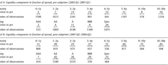
5t is the 5% quantile of the liquidity measure. The liquidity component is then divided by the bond’s yield spread and within each group we find the median liquidity fraction. We show inAppendix Bthat the size of the liquidity component is robust to the choice of benchmark riskfree rate, but the liquidity fraction of the total spread is sensitive to the benchmark. The swap Table 4

Liquidity component in basis points.

For each ratingR, we run the pooled regression

SpreadR

it¼aRþbRlitþCredit risk controlsitþEit,

whereirefers to bond,tto time, andlitis our liquidity measure. The bond spread is measured with respect to the swap rate. Within each rating and maturity bucket (0–2y, 2–5y, and 5–30y), we sort increasingly all values oflitand find the median valuel50and the 5% valuel5. The liquidity component in the bucket is defined asbðl50l5Þ. This table shows for all buckets the liquidity component with standard errors in parentheses. Confidence bands are found by a wild cluster bootstrap. The data are U.S. corporate bond transactions from TRACE and the sample period is from 2005:Q1 to 2009:Q2.

Panel A: Liquidity component in basis points, pre-subprime(2005Q1–2007:Q1)

Average Liquidity component, basis points Number of observations

0–2y 2–5y 5–30y 0–2y 2–5y 5–30y

AAA 0.8 0:6 ð0:3;0:8Þ ð0:05:;91:3Þ ð01:6:;11:5Þ 162 178 193 AA 1.0 0:7 ð0:3;1:1Þ ð0:14:;01:7Þ ð01:5:;23:2Þ 704 667 498 A 2.4 1:5 ð0:6;2:3Þ ð1:21:;53:9Þ ð13:4:;42:9Þ 1540 1346 1260 BBB 3.9 2:8 ð1:4;4:4Þ ð1:49:;06:2Þ ð24:3:;77:3Þ 517 270 553 Spec 57.6 45:0 ð32:3;57:4Þ ð3144:5;:560:0Þ ð6083:2;106:9:8Þ 270 324 480

Panel B: Liquidity component in basis points, post-subprime(2007:Q2–2009:Q2)

Average Liquidity component, basis points Number of observations

0–2y 2–5y 5–30y 0–2y 2–5y 5–30y

AAA 4.9 2:5 ð0:5;4:4Þ ð0:49:;85:0Þ ð1:77;:149:1Þ 110 149 155 AA 41.8 23:5 ð12:9;33:2Þ ð2037:3;52:1:4Þ ð3564:5;91:7:4Þ 493 572 483 A 50.7 26:6 ð15:3;39:2Þ ð2951:3;75:0:1Þ ð4274:9;109:5:7Þ 762 878 890 BBB 92.7 64:3 ð36:5;92:7Þ ð65115:6;166:6:6Þ ð5598:7;141:1:4Þ 123 159 256 Spec 196.8 123:6 ð80:2;157:3Þ ð145224:3;285:0:1Þ ð157242:4;308:7:8Þ 133 129 201 8

Longstaff, Mithal, and Neis (2005) find an average nondefault component of -7.2bp for AAA/AA, 10.5bp for A, and 9.7bp for BBB,Han and Zhou (2008)find the nondefault component to be 0.3bp for AAA, 3.3bp for AA, 6.7bp for A, and 23.5bp for BBB, whileBlanco, Brennan, and Marsh (2005)find it to be 6.9bp for AAA/AA, 0.5bp for A, and 14.9bp for BBB.

9

Longstaff, Mithal, and Neis (2005)report an average of 17.6bp for BB, whileHan and Zhou (2008)estimate it to be 2.8bp for BB,53.5bp for B, and75.4bp for CCC.

rate is chosen because there is mounting evidence that swap rates are better proxies for riskfree rates than Treasury yields (see, for example, Hull, Predescu, and White, 2004;Feldh ¨utter and Lando, 2008).

Table 5shows the fraction of the liquidity component to the total corporate-swap spread. The first parts of Panels A and B sort according to rating. We see that the fraction of spreads due to illiquidity is small for investment grade bonds, 11% or less. Using the ratio of the swap basis relative to the total spread, Longstaff, Mithal, and Neis (2005) find the fraction of spread due to liquidity at the 5-year maturity to be 2%, whileHan and Zhou (2008)find it to be 19% consistent with our finding that it is relatively small. In speculative grade bonds the fraction due to liquidity is 24%. Post-subprime, the fractions increase and range from 23% to 42% in all ratings but AAA where it is only 7%. That the liquidity fractions of spreads in AAA are small in percent relative to other bonds underscores that there is a flight-to-quality effect in AAA bonds. A consistent finding fromTables 4 and 5 is that for investment grade bonds the importance of liquidity has increased after the onset of the subprime crisis both in absolute size (basis points) and relative to credit risk (fraction of spread). For speculative grade bonds the liquidity component in basis points has increased but it is stable measured as the fraction of total yield spread.

The last parts of Panels A and B inTable 5show the liquidity fraction of total spread as a function of maturity. We introduce a fine maturity grid but do not sort accord-ing to rataccord-ing to have a reasonable sample size in each bucket. We see that the fraction of the spread due to liquidity is small at short maturities and becomes larger as maturity increases. This is the case both pre- and post-subprime, although the fraction is higher post-subprime for all maturities. For example, post-subprime, the

fraction of spread due to liquidity is 43% for bonds with a maturity more than ten years while it is 11% for maturities less than one year. The fraction increases at maturities shorter than five years and thereafter flattens. The slight dip at the 8–10y maturity both pre- and post-subprime is due to an on-the-run effect; many bonds are issued with a maturity of ten years and are more liquid right after issuance.10

We find strong differences in the pre- and post-subprime periods, and to examine the variation within the two periods more closely, we estimate monthly variations in liquidity and spreads as follows. Each month we (a) find a regression coefficient

b

t by regressing spreads on

l

while controlling for credit risk, (b) calculate for each bond the fraction due to illiquidity,

b

tð

l

it

l

5tÞ=spreadit, (c) find the median fraction, and (d) multiply this fraction by the median spread. This gives us the total liquidity premium in basis points on a monthly basis. We do this for investment grade and spec-ulative grade bonds separately.11_{This measures the amount}

of the total spread that is due to illiquidity.Fig. 3shows the time-series variation in the median spread and the amount of the spread due to illiquidity.

The liquidity premium in investment grade bonds is persistent and steadily increasing during the subprime crisis and peaks in the first quarter of 2009 when stock prices decreased strongly. We see that the co-movement between the liquidity premium and credit spread is quite high. For Table 5

Liquidity component in fraction of spread. For each ratingR, we run the pooled regression

SpreadR

it¼aRþbRlitþCredit risk controlsitþEit,

whereirefers to bond,tto time, andlitis our liquidity measure. Within each rating we sort increasingly all values oflitand find the 5% valuel5. For each bond we define the liquidity fraction of the total spread asbRðlitl5Þ=SpreadRit. The estimated fractions in the table are for each entry the median fraction. Confidence bands are found by a wild cluster bootstrap. The data are U.S. corporate bond transactions from TRACE and the sample period is from 2005:Q1 to 2009:Q2.

Panel A: Liquidity component in fraction of spread, pre-subprime(2005:Q1–2007:Q1)

Maturity 0–1y 1–2y 2–3y 3–4y 4–5y 5–8y 8–10y 10–30y

Fraction in pct 3

ð2;4Þ ð47;9Þ ð813;17Þ ð813;18Þ ð813;17Þ ð711;15Þ ð58;11Þ ð710;14Þ

Number of observations 1596 1613 1241 891 641 1187 578 1218

Rating AAA AA A BBB Spec

Fraction in pct 3

ð2;5Þ ð24;7Þ ð511;18Þ ð38;12Þ ð1824;30Þ

Number of observations 533 1869 4148 1340 1075

Panel B: Liquidity component in fraction of spread, post-subprime(2007:Q2–2009:Q2)

Maturity 0–1y 1–2y 2–3y 3–4y 4–5y 5–8y 8–10y 10–30y

Fraction in pct 11

ð7;14Þ ð1320;27Þ ð1523;31Þ ð1827;38Þ ð2031;42Þ ð2844;60Þ ð2133;44Þ ð2843;53Þ

Number of observations 809 819 675 657 556 817 568 598

Rating AAA AA A BBB Spec

Fraction in pct 7

ð1;12Þ ð2342;60Þ ð1426;39Þ ð1629;41Þ ð1623;30Þ

Number of observations 414 1549 2533 539 464

10_{To support this claim, we additionally sorted according to bond} age (older and younger than two years). After this sort, the dip at the 8–10y maturity was not present. Results are available on request.

11

The results become unstable if we split into finer rating cate-gories. While the quantiles oflcan be determined reasonably well, the regression coefficientbRt becomes noisy.

speculative grade bonds, the liquidity premium peaks around the bankruptcy of Lehman and shows less persis-tence. Furthermore, the co-movement between the liquidity premium and the spread is less pronounced than for investment grade bonds, and the premium at the end of the sample period is almost down to pre-crisis levels even though the spread is still higher than before the crisis.

5. Determinants of bond illiquidity

In this section, we use our measure of liquidity to document some key mechanisms by which corporate bond

illiquidity is affected. Specifically, we focus on the liquidity of bonds with a lead underwriter in financial distress, the liquidity of bonds issued by financial firms relative to bonds issued by industrial firms, and liquidity betas.

5.1. Lead underwriter

Brunnermeier and Pedersen (2009)provide a model that links an asset’s market liquidity and traders’ funding liquid-ity, and find that when funding liquidity is tight, traders become reluctant to take on positions, especially ‘capital intensive’ positions in high-margin securities. This lowers

Apr05 Jul05 Oct05 Jan06 Apr06 Jul06 Oct06 Jan07 Apr07 Jul07 Oct07 Jan08 Apr08 Jul08 Oct08 Jan09 Apr09 0 1 2 3 4 5 Spread in percent Investment grade

Apr05 Jul05 Oct05 Jan06 Apr06 Jul06 Oct06 Jan07 Apr07 Jul07 Oct07 Jan08 Apr08 Jul08 Oct08 Jan09 Apr09 0 5 10 15 20 25 30 Spread in percent Speculative grade Spread Liquidity premium Spread Liquidity premium

Fig. 3.Liquidity premium and total spread for investment grade and speculative grade bonds. This graph shows for investment grade and speculative

grade yield spreads the variation over time in the amount of the spread that is due to illiquidity and the total yield spread. On a monthly basis, the fraction of the yield spread that is due to illiquidity is calculated as explained inSection 4.3. This fraction multiplied by the median yield spread is the amount of the spread due to illiquidity and plotted along with the median yield spread. The data are U.S. corporate bond transactions from TRACE and the sample period is from 2005:Q1 to 2009:Q2.

market liquidity. Empirical support for this prediction is found inComerton-Forde, Hendershott, Jones, Moulton, and Seasholes (2010)who find for equities traded on NYSE that balance sheet and income statement variables for market makers explain time variation in liquidity.

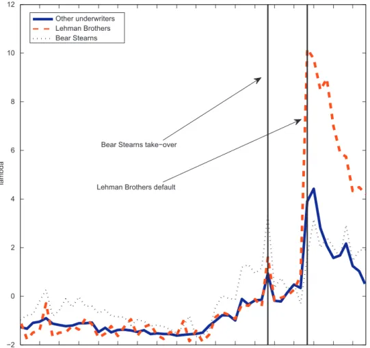
Since the TRACE data do not reveal the identity of the traders, we cannot perform direct tests of theBrunnermeier and Pedersen (2009)-model for the U.S. corporate bond market. However, if we assume that the original under-writer is more likely to make a market as is the case in equity markets, seeEllis, Michaely, and O’Hara (2000), we can provide indirect evidence by observing bond liquidity of bonds underwritten by Bear Stearns and Lehman Brothers, two financial institutions in distress during the subprime crisis. We therefore calculate for all bonds with Lehman Brothers as lead underwriter their average

l

—weighted by amount outstanding—on a monthly basis. Likewise, we do this for bonds with Bear Stearns as lead underwriter and for all other bonds that are not included in the Bear Stearns and Lehman samples. We obtain underwriter information from

the Fixed Income Securities Database (FISD). The results are plotted inFig. 4.

The liquidity of bonds with Bear Stearns as lead under-writer was roughly the same as an average bond entering in the summer of 2007. During the week of July 16, 2007, Bear Stearns disclosed that two of their hedge funds had lost nearly all of the value, and the graph shows that the ‘illiquidity gap’ between Bear Stearns underwritten bonds and average bonds increased that month. On August 6, Bear Stearns said that it was weathering the worst storm in financial markets in more than 20 years, in November 2007 Bear Stearns wrote down $1.62 billion and booked a fourth quarter loss, and in December 2007 there was a further write-down of $1.90 billion. During these months, the ‘illiquidity gap’ steadily increased. Bear Stearns was in severe liquidity problems in the beginning of March, and they were taken over by JP Morgan on March 16. In this month the ‘illiquidity gap’ peaked but returned to zero in June 2008 after Bear Stearns shareholders approved JP Morgan’s buyout of the investment bank on May 29.

Jan05 Apr05 Jul05 Oct05 Jan06 Apr06 Jul06 Oct06 Jan07 Apr07 Jul07 Oct07 Jan08 Apr08 Jul08 Oct08 Jan09 Apr09 −2 0 2 4 6 8 10 12

Bear Stearns take−over

Lehman Brothers default

lambda

Other underwriters Lehman Brothers Bear Stearns

Fig. 4.Illiquidity of bonds underwritten by Lehman Brothers and Bear Stearns. This graph shows the time-series variation in illiquidity of bonds with

Lehman Brothers as lead underwriter, bonds with Bear Stearns as lead underwriter, and the rest of the sample. The data are U.S. corporate bond transactions from TRACE and the sample period is from 2005:Q1 to 2009:Q2. For every bond underwritten by Lehman Brothers, their (il)liquidity measurelis calculated each month and a monthly weighted average is calculated using amount outstanding for each bond as weight. The graph shows the time series of monthly averages. Likewise, a time series of monthly averages is calculated for bonds with Bear Stearns as a lead underwriter and for all bonds that are not included in the Lehman and Bear Stearns samples. Higher values on they-axis imply more illiquid bonds.

In particular, this buyout meant that JP Morgan assumed Bear Stearns’ trading business, and the ‘illiquidity gap’ returning to zero is consistent with the market’s perception of JP Morgan as being well-capitalized.

The liquidity of bonds underwritten by Lehman was close to the liquidity of an average bond in the market up until August 2008, but this changed when the ‘illiquidity gap’ between Lehman underwritten bonds and average market bonds increased strongly in response to Lehman filing for bankruptcy on September 15. On September 17, Barclays announced that it acquired Lehman’s North American trading unit. The gap stayed at high levels during the rest of the sample period showing that after the Lehman default, bonds they had underwritten became permanently more illiquid. This suggests that a bank-ruptcy (Lehman) has a permanent effect on the illiquidity of underwritten bonds while a takeover (Bear Stearns) has a temporary effect. The permanent effect caused by bank-ruptcy might be because the default left Barclays with more pressing issues after the acquisition than resuming market-making activities linked to underwritten bonds. Another contributing factor could be that a counterparty with which Lehman had a relationship as broker was more likely to hold bonds underwritten by Lehman. These bonds might be held by Lehman as collateral if Lehman financed the counterparty. After the default the collateral could not easily be returned, as explained inAragon and Strahan (in press), and therefore could not be traded by the counter-party leading to a loss in market liquidity in that bond.

Aragon and Strahan (in press) study hedge funds with a broker relationship with Lehman. Consistent with our find-ings, they find (a) a permanent loss in liquidity of assets traded by these hedge funds after the Lehman default, and (b) no permanent effect during the Bear Stearns takeover in the case of Bear Stearns being the broker.12

5.2. Industry

The yield spreads on bonds issued by financial firms peaked around key events of the subprime crisis. Concerns about the credit quality of financial firms were of course a main driver behind these spread widenings, but it is con-ceivable that deteriorating liquidity of their bond issues was also a factor. We address this issue by calculating an average (weighted by amount outstanding) monthly

l

of financial and industrial firms, respectively, and plotting the time-series behavior inFig. 5. We obtain bond issuer character-istics from FISD.

In general, there is little systematic difference. For both financial and industrial bonds, illiquidity goes up at the onset of the crisis. There are, however, additional spikes in illiquid-ity for financial firms around the takeover of Bear Stearns in March 2008, around the Lehman bankruptcy in September 2008, and around the stock market decline in the first

quarter of 2009. That is, in times of severe financial distress, illiquidity of financial bonds increases relative to that of industrial bonds, while in other times liquidity is similar. This pattern might be due to the heightened information asym-metry regarding the state of the financial firms—including their financial linkages—around the dramatic events.

By calculating monthly averages, we are able to draw more high-frequency inferences compared to Longstaff, Mithal, and Neis (2005)and Friewald, Jankowitsch, and Subrahmanyam (forthcoming). If we average

l

over longer periods of time, as in the approach taken in those two papers, the effects we find would be washed out. Our results therefore reconcile the finding inLongstaff, Mithal, and Neis (2005)that bonds issued by financial firms are more illiquid with the finding inFriewald, Jankowitsch, and Subrahmanyam (forthcoming) that there is no sys-tematic liquidity difference.

5.3. Liquidity betas

We estimate bond-specific liquidity betas by calculat-ing a monthly time series of corporate bond market illiquidity, and for each bond estimate the correlation between market-wide illiquidity and bond-specific illi-quidity. The market-wide time series is calculated by averaging on a monthly basis across all observations of bond-specific

l

i using amount outstanding as weight. Bond-specific beta is estimated through the slope coeffi-cient in the regression of bond-specific

l

ion market-wide

l

, where the regression is based on all months where a bond-specific

l

ican be calculated. We calculate the betas using the whole sample period 2005Q1–2009Q2, because estimating betas separately for the pre- and post-sub-prime periods leads to noisier estimates. Once we have estimated a liquidity beta using the complete sample period, we examine the dependence of spreads on this beta in the two subperiods.

For each rating class R, pooled regressions are run where yield spreads are regressed on each bond’s liquidity

b

and our liquidity measure

l

twith credit risk controls: SpreadRit¼

a

R þ

g

R

1

l

itþ

g

R2

b

iþCredit risk controlsitþ

Eit

, whereiis for bond in ratingRandtis time measured in quarters.

The result of the regression is reported inTable 6. Our regressions are run both ‘marginally’, i.e., with the liquid-ity beta as the only regressor in addition to the credit risk controls, and with our liquidity measure included as an additional regressor.

Both marginally and with

l

included, there is no significance pre-subprime except for the AAA-category. After the onset of the crisis, the picture changes and only spreads in the AAA-category do not depend on the liquidity beta. This is consistent with the regime-depen-dent importance of liquidity betas noted in Acharya, Amihud, and Bharath (2010). But whereas they use stock and Treasury bond market liquidity to measure aggregate liquidity, our measure specifically captures corporate bond market liquidity.

We saw in the previous section that the contribution to spreads of liquidity was small for AAA bonds after the 12_{In results not reported we have also looked at bonds}

under-written by Merrill Lynch. In these bonds there is an increase in illiquidity relative to other bonds in the months leading up to September 2008 when Merrill Lynch was taken over by Bank of America. After the takeover, this ‘run-up’ disappears so the effect is temporary as in the Bear Stearns case. A graph is available on request.

onset of the crisis, and the insignificant liquidity beta coefficient for AAA in the crisis period confirms that there is a flight-to-quality effect in AAA-rated bonds.

6. Robustness checks

InAppendix Bwe carry out a series of robustness checks. We test for potential endogeneity bias and find that endo-geneity is not a major concern. We calculate liquidity premia using corporate bond spreads to Treasury rates instead of swap rates and find that our conclusions still hold. And we examine an alternative definition of our liquidity component and find results to be robust to this definition.

As a further test showing that our regression results are robust, we employ a different methodology for con-trolling for credit risk. The idea is that any yield spread difference between two fixed-rate bullet bonds with the same maturity and issued by the same firm must be due to liquidity differences and not differences in credit risk. This intuition is formalized in the following regression. We conduct rating-wise ‘paired’ regressions of yield

spreads on dummy variables and one liquidity measure at a time. The regression is

SpreadRit¼Dummy

R Gtþ

b

R

l

itþ

Eit

,

whereDummyRGtis the same for all bonds with the same ratingRand approximately the same maturity. The grid of maturities is 0–0.5y, 0.5–1y, 1–3y, 3–5y, 5–7y, 7–10y, and more than 10y. For example, if firmiin quarterthas three bonds issued with maturities 5y, 5.5y, and 6y, the bonds have the same dummy in that quarter, and we assume that any yield spread difference between the bonds is due to liquidity. There are separate dummies for each quarter. Once we have dummied out credit risk in the regressions, estimated coefficients for the liquidity measure are not inconsistent because of possibly omitted credit risk variables. Hence, the paired regression is free of any endogeneity bias due to credit risk. Only groups with two or more spreads contribute to the liquidity coefficient reducing the sample compared to former regressions. Therefore, we only look at two rating groups, investment grade and speculative grade.Table 7shows the regression

Jan05 Apr05 Jul05 Oct05 Jan06 Apr06 Jul06 Oct06 Jan07 Apr07 Jul07 Oct07 Jan08 Apr08 Jul08 Oct08 Jan09 Apr09 −2 −1 0 1 2 3 4 lambda

Bonds of industrial firms Bonds of financial firms

Fig. 5. Illiquidity of bonds of industrial and financial firms. This graph shows the time-series variation in illiquidity of bonds of industrial and financial

firms. The data are U.S. corporate bond transactions from TRACE and the sample period is from 2005:Q1 to 2009:Q2. For every bond issued by a financial firm, their (il)liquidity measurelis calculated each month and a monthly weighted average is calculated using amount outstanding for each bond as weight. The graph shows the time series of monthly averages. Likewise, a time series of monthly averages is calculated for bonds issued by industrial firms. Higher values on they-axis imply more illiquid bonds.

coefficients in the paired regression. We see that

l

is significant for both investment grade and speculative grade bonds in the period before the subprime crisis as

well as after the onset of the crisis. This supports our finding that

l

is successful at disentangling liquidity and credit risk.

To address the potential concern that our results are confounded by an increase of new issues towards the end of the sample period, we calculate the average age of the bonds in the sample on a monthly basis. We find no trend during the sample period which suggests that our results are not driven by an increase in bond issues (results are available on request). We also recalculate the total spread and liquidity premium in Fig. 3 using only bonds in existence by February 2005.13 _{The reduction in the}

sample leads to increased noise in our results. To make it clear how this noise affects our results, we redo the calculations in two different ways. Recall that for each bond, the fraction due to illiquidity is calculated as

b

tð

l

it

l

5tÞ=Spreadit, where

b

t is the liquidity regression

coefficient in month t,

l

it is the bond-specific liquidity level in montht,Spreaditthe bond-specific spread, and

l

5tis the 5% liquidity quantile in montht. In the first recalcula-tion, we assume that the sensitivities of spreads to illiquid-ity are not influenced by a potential issuance effect, but that the overall level of illiquidity might be effected. Specifically, we use the regression coefficients

b

tobtained using the full sample, while calculating

l

it, Spreadit, and

l

5t using the reduced sample (bonds in existence by February 2005).

Fig. 6shows the results along with those inFig. 3(‘results in the paper’, respectively, ‘reduced sample, fixed reg. coeff.’). There is little difference in the results, so results based on

l

are robust to using only bonds issued by February 2005. In particular, this implies that our results on underwriter and financial vs. industrial firms are robust to a possible issu-ance effect. In our second recalculation, we also recalculate the regression coefficients

b

tusing only bonds in existence by February 2005. That is, we redo the whole analysis with the reduced sample. The results are also inFig. 6marked ‘reduced sample’. (Note that the yield spreads are the same for the ‘reduced sample, fixed reg. coeff.’ and ‘reduced sample’ methods.) We see that results become more noisy, in particular for speculative grade bonds. For example, the liquidity component for speculative grade bonds in Novem-ber 2008 is small. However, the results still show that the spike and subsequent decline in high yield spreads to a certain extent was a liquidity issue.

7. Conclusion

The subprime crisis dramatically increased corporate bond spreads and it is widely believed that deteriorating liquidity contributed to the widening of spreads.

We use a new measure of illiquidity—derived from a principal component analysis of eight liquidity proxies—to analyze the contribution of illiquidity to corporate bond spreads. The measure outperforms the Roll measure used in

Bao, Pan, and Wang (2011)and zero-trading days used in

Chen, Lesmond, and Wei (2007)in explaining spread varia-tion. In fact, the number of zero-trading days tends to Table 6

Beta regressions.

For each rating classR, pooled regressions are run where yield spreads are regressed on each bond’s liquidityband our liquidity measurelt with credit risk controls:

SpreadRit¼aRþgR1litþgR2biþCredit risk controlsitþEit,

whereiis for bond in ratingRandtis time measured in quarter. Each bond’sbiis calculated as the covariance between this bond’s monthlylit and a size-weighted monthly marketlMt. Two regressions for each rating pre- and post-subprime are run; one with onlybincluded and one with bothbandlincluded. The pre-subprime period is 2005:Q1–2007:Q1 while the post-subprime period is 2007:Q2–2009:Q2. The data are U.S. corporate bond transactions from TRACE. Standard errors are corrected for time-series effects, firm fixed effects, and heteroskedasticity, and significance at 10% level is markedn , at 5% markednn , and at 1% markednnn . Pre-subprime Post-subprime b l b l AAA 0:0034 ð1:34Þ 0:0085 ð0:84Þ 0:0056nnn ð3:26Þ 0:0033 nnn ð2:65Þ 0 :0159 ð1:26Þ 0:0234 nn ð2:38Þ AA 0:0012 ð0:23Þ 0:1823 n ð1:94Þ 0:0067 ð1:06Þ 0:ð00170:60Þ 0:1720 nn ð2:14Þ 0:1712 nnn ð3:82Þ A 0:0004 ð0:14Þ 0:2631 nn ð2:22Þ 0:0021 ð0:65Þ 0:0106 nn ð2:57Þ 0:2314 nn ð2:15Þ 0:1211 nn ð2:03Þ BBB 0:0044 ð1:34Þ 0:2171 nnn ð4:05Þ 0:0012 ð0:34Þ 0:0254 nnn ð4:33Þ 0:3187 nnn ð3:44Þ 0:3242 nnn ð2:91Þ Spec 0:0102 ð0:90Þ 1:3538 nnn ð2:60Þ 0:0162 ð1:31Þ 0:1502 nnn ð4:64Þ 1:3140 nn ð2:73Þ 0:4155 nnn ð7:08Þ Table 7 Paired regression.

We pair bonds from the same firm with similar maturity and regress their yield spreads on liquidity variables one at a time and add a dummy for a given firm and maturity combination. Since bonds with similar maturity and issued by the same firm have similar credit risk character-istics, the dummy controls for credit risk. Significance at 10% level is markedn

, at 5% markednn

, and at 1% markednnn

. The data are U.S. corporate bond transactions from TRACE and the sample period is from 2005:Q1 to 2009:Q2.

Pre-subprime Post-subprime Investment Speculative Investment Speculative

l 0:01nnn ð3:79Þ 0:09 nn ð2:43Þ 0:12 nnn ð3:58Þ 0:41 n ð1:95Þ Amihud 2:26nnn ð5:11Þ 16:80 nnn ð3:51Þ 16:10 nnn ð3:04Þ 54:65 ð1:54Þ Roll 0:03nnn ð3:56Þ 0:16 nn ð2:54Þ 0:05 nn ð2:14Þ 0:39 ð1:44Þ Bond zero 0:00nnn ð5:85Þ 0:01 nn ð2:28Þ 0:00 ð0:78Þ 0ð1::0312Þ Turnover 0:11n ð1:87Þ 1:48 n ð1:72Þ 3:21 ð1:46Þ 72ð1::6374Þ IRC 8:48nnn ð3:72Þ 125:03 nn ð2:55Þ 104:34 nn ð2:43Þ 95:04 ð0:58Þ IRC risk 1:30 ð0:69Þ 57:15 nn ð2:15Þ 39:09 nnn ð2:97Þ 103:42 ð0:74Þ Amihud risk 0:64nnn ð4:21Þ 9:44 nnn ð2:79Þ 6:56 nnn ð3:19Þ 39:63 nnn ð4:60Þ 13

decrease during the crisis, because trades in less liquid bonds are split into trades of smaller size.

Before the crisis, the contribution to spreads was small for investment grade bonds both measured in basis points and as a fraction of total spreads. The contribution increased strongly at the onset of the crisis for all bonds except AAA-rated bonds, which is consistent with a flight-to-quality into AAA-rated bonds. Liquidity premia in

investment grade bonds rose steadily during the crisis and peaked when the stock market declined strongly in the first quarter of 2009, while premia in speculative grade bonds peaked during the Lehman default and returned almost to pre-crisis levels in mid-2009.

Our measure is useful for analyzing other aspects of corporate bond liquidity. We show that the financial distress of Lehman and Bear Stearns diminished the

Apr05 Jul05 Oct05 Jan06 Apr06 Jul06 Oct06 Jan07 Apr07 Jul07 Oct07 Jan08 Apr08 Jul08 Oct08 Jan09 Apr09 0 1 2 3 4 5 Spread in percent Investment grade

Apr05 Jul05 Oct05 Jan06 Apr06 Jul06 Oct06 Jan07 Apr07 Jul07 Oct07 Jan08 Apr08 Jul08 Oct08 Jan09 Apr09 0 5 10 15 20 25 30 35 Spread in percent Speculative grade

Spread, full sample Spread, reduced sample Liquidity premium, full sample

Liquidity premium, reduced sample, fixed reg. coeff. Liquidity premium, reduced sample

Spread, full sample Spread, reduced sample Liquidity premium, full sample

Liquidity premium, reduced sample, fixed reg. coeff. Liquidity premium, reduced sample

Fig. 6.Liquidity premium and total spread for investment grade and speculative grade bonds using only bonds in existence by February 2005. On a

monthly basis, the fraction of the yield spread that is due to illiquidity is calculated asbtðlitl5tÞ=Spreadit(as explained inSection 4.3. This fraction multiplied by the median yield spread is the amount of the spread due to illiquidity and plotted along with the median yield spread. ‘Full sample’ refers to the results inFig. 3. ‘Reduced sample’ refers to results using a sample restricted to bonds in existence by February 2005. ‘Reduced sample, fixed reg. coeff.’ refers to results wherebtis calculated using the full sample whilelitl5tis calculated using the reduced sample. The data are U.S. corporate bond transactions from TRACE and the sample period is from 2005:Q1 to 2009:Q2.